Visual cortex frontend: integrating lines, edges, keypoints and disparaty

integrating lines, edges, keypoints and disparity

1 _{University of Algarve - Escola Superior Tecnologia, Faro, Portugal} 2 _{University of Algarve - Vision Laboratory - FCT, Faro, Portugal}

Abstract. We present a 3D representation that is based on the pro-cessing in the visual cortex by simple, complex and end-stopped cells. We improved multiscale methods for line/edge and keypoint detection, including a method for obtaining vertex structure (i.e. T, L, K etc). We also describe a new disparity model. The latter allows to attribute depth to detected lines, edges and keypoints, i.e., the integration results in a 3D “wire-frame” representation suitable for object recognition.

1

Introduction

During the last decade, the modeling of processes in the visual cortex has become a mature research topic. Models of cells, i.e. simple, complex and end-stopped, have been developed, e.g. [5, 17]. In addition, models of bar and grating cells [12, 13], line/edge detection [4, 7, 8, 16] and disparity [3, 11] have become avail-able. Hence, it is now possible to develop a vision frontend that integrates all types of processing and that can be used to explore higher-level tasks like object recognition.

The basic syntax in the primary cortex seems to consist of lines (bars) and edges, also keypoints, in scale space. However, there is more going on: because of the ocular dominance columns in the primary cortex [6], which bring retinotopic, orientation-specific projections of the left and right eye closely together such that neural dendritic fields can cover both, we must assume that disparity estimation already starts at the first processing layers [18].

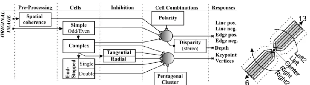
We present a 3D “wire-frame” representation based on an integrated fron-tend (Fig. 1 left) which allows to detect positive and negative lines and edges, keypoints, vertex structure and depth. We also present a new disparity model that is not based on phase [3] nor amplitude summations [11]. The basic idea is extremely simple: once we have line/edge detection, we also have access to the central, linear part of the Gabor responses. Below we first introduce keypoints with stabilizations and the new method for underlying vertex structure, then line/edge extraction with stabilizations, and finally the new disparity model.

2

Simple, complex and end-stopped cells

Line, edge and keypoint detection are based on the responses of simple, complex and end-stopped cells. Gabor quadrature filters provide a model of cortical simple

(Nθ= 8 in our case). We apply a linear scaling between fminand fmax, with the possibility of using many contiguous scales or a few noncontiguous scales with neighboring micro-scales.

In the spatial domain, the responses of even and odd simple cells, which correspond to the real and imaginary parts of the Gabor filters, are denoted by

RE

s,i(x, y) and ROs,i(x, y), s being the scale and i the orientation (i.e. θi ⊥ ρi

and θi= iπ/(Nθ− 1)). In order to simplify the notation, and because the same

processing is done at all scales, we drop the subscript s. The responses of complex cells are modelled by the modulus Ci(x, y) = [{REi (x, y)}2+ {ROi (x, y)}2]1/2.

There are two types of end-stopped cells [5, 17], i.e. single (S) and double (D). If [·]+ _{denotes the suppression of negative values, C}

i= cos θi and Si= sin θi, then

Si(x, y) = [Ci(x + dSi, y − dCi) − Ci(x − dSi, y + dCi)]+; Di(x, y) = · Ci(x, y) − 1 2Ci(x + 2dSi, y − 2dCi) − 1 2Ci(x − 2dSi, y + 2dCi) ¸+ .

The distance d is scaled linearly with the filter scale s, i.e. d = 0.6s. All end-stopped responses along straight lines and edges need to be suppressed, for which we use tangential (T) and radial (R) inhibition:

IT(x, y) = 2NXθ−1 i=0 [−Ci mod Nθ(x, y) + Ci mod Nθ(x + dCi, y + dSi)] + ; IR_{(x, y) =} 2NXθ−1 i=0 ·

Ci mod Nθ(x, y) − 4 · C(i+Nθ/2) mod Nθ(x +

d 2Ci, y + d 2Si) ¸+ ,

where (i+Nθ/2) mod Nθ⊥ i mod Nθ. Instead of applying the inhibition to

indi-vidual end-stopped cells [5, 17], slightly better results are obtained by applying

I = IT_{+ I}R _{once to the pooled activity:}

KS_{(x, y) =} NXθ−1 i=0 Si(x, y) − gI(x, y) and KD(x, y) = NXθ−1 i=0 Di(x, y) − gI(x, y),

with g ≈ 0.4, after which the keypoint map is obtained: K(x, y) = max{KS_{(x, y),}

KD_{(x, y)}, i.e. at each filter scale s: K} s(x, y).

This cell model leads to the detection of many spurious events. The main reason for this problem lies in the Gabor filtering itself: at an L junction the

Fig. 1. Left: integrated frontend (see text); right: pentagonal cell clusters.

filters respond beyond the line/edge parts, and non-ideal edges lead to shifts of the even and/or odd responses parallel to the “edge center.” For this reason the accuracy must be improved by postprocessing, and a further stabilization can be achieved by combining detection at multiple scales.

3

Keypoint stabilization and vertex classification

For pattern recognition applications we want to obtain a clean, single-pixel key-point map, and classify the keykey-points according to the underlying vertex struc-ture, i.e. K, L, T, + etc. All postprocessing of K(x, y) is done in four steps, for each scale, after which different scales are combined.

First, local maxima of K(x, y) in x and y are detected. If there is a small cluster of connected points with equal values, the centroid will be computed.

Second, for each local maximum (centroid) the responses of the complex cells

Ci(x, y) are analyzed in order to keep the dominant orientations θi: we mark

all orientations for which (a) Ci > Ci−1∧ Ci > Ci+1, where i is cyclic over

0 and Nθ− 1, and (b) Ci exceeds a threshold value of 0.05 · CPA. CPA is the average of all complex cell responses pooled over a 3 × 3 neighborhood and all orientations: CPA = 1/9 ·

P

3×3CP and CP =

PNθ−1

i=0 Ci. Then, the number of

dominant orientations are counted in a 9 × 9 neighborhood, and those with a count less than 0.05 of the total count are discarded.

Third, in the case of e.g. T and L vertices the complex cells respond beyond the keypoints in dominant orientations, so now we need to analyze opposite

di-rections. Insignificant directions are eliminated by probing the dominant

orien-tations on a line in opposite directions starting at the local maximum (centroid), until a distance of d1which is linearly scaled with the filter scale. If the number of dominant orientations found is below d1/2, directions are rejected.

Fourth, probed and passed directions are further confirmed by analyzing the dominant orientations, now with three pentagonal cell clusters used for each probed direction (width w and length d1, we use 3 and 6 respectively).

All the constants and mask sizes depend on filter scale (i.e. are scaled lin-early). Figure 1 (right) shows the central pentagonal cluster (shaded) and shifted ones (orthogonally ±1 pixel, dark outline) for directions 6 and 13. Only those directions are kept which have consistent dominant orientations in at least one

and these are labelled with the line/edge directions, i.e., the vertex type (K, L, T, + etc.) is also available (see Fig. 2 bottom-left).

In a final step the keypoint stability in scale space is confirmed by considering, around each scale, a small scale interval: 4 micro-scales, i.e. two scales slightly finer and two slightly coarser than the actual scale. In the case of the smallest (largest) scale, four coarser (finer) scales are applied. Only keypoints which are consistent over 3 neighboring micro-scales are accepted.

4

Line/edge stabilization and classification

Van Deemter and du Buf [16] presented a scheme for line and edge detection based on the responses of simple cells. A positive line is detected where RE

shows a local maximum in the orthogonal filter orientation and RO_{shows a zero}

crossing. In the case of an edge the even and odd responses must be swapped. This gives 4 possibilities for positive and negative events: local maxima/minima plus zero crossings. Here we combine the responses of simple and complex cells, i.e. simple cells serve to detect positions and event types, whereas complex cells are used to increase the confidence. Since the use of Gabor modulus (complex cells) implies some loss of precision at vertices [2] we increase precision by considering multiple scales.

For each orientation the simple cells responses (RE

i or ROi ) orthogonal to

the orientation are checked for a local maximum (or minimum), until a distance of ±λ/4, λ being the wavelength of the Gabor filter. All positions that do not show a local maximum (minimum) are discarded. Then complex cells (Ci) are

checked, using the same process. Only at positions that pass the previous tests the quadrature filter is checked for a zero crossing on ±λ/4. If so, the position is accepted and the event type has been determined (Fig. 2 top-right, where four different colors represent the line/edge events).

Finally, polarity and spatial coherence are checked. Event polarity must be corrected when, due to interference effects, the Gabor responses are distorted. We correct individual points of lines and edges if their polarity differs from that of the neighboring points. Spatial coherence is improved by suppressing all events at positions where the local variance of the input image is too low. This is necessary to suppress line/edge events beyond keypoints in insignificant directions (e.g. at L and T junctions). As is done in the case of keypoints, the coherence is also improved by checking the results at 4 neighboring micro-scales.

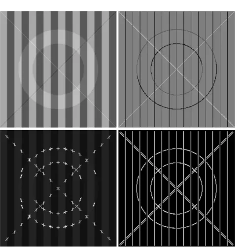
Fig. 2. Ledge image (top-left), line/edge detection (top-right), keypoints with vertex structure (bottom-left). For comparison, the result of Canny’s edge operator is shown bottom-right.

5

Disparity estimation

Our new disparity model is based on the central, linear part of the Gabor re-sponses, i.e. the sinusoidal part with sin x ≈ x, |x| < π/4. Assuming ideal events, i.e. lines with a Dirac profile and edges with a Heaviside step profile, or nonideal ones obtained by Gaussian filtering, and complex Gabor filters with the same ori-entation, the responses are (scaled) Gabor functions and complex errorfunctions. It has been shown that the latter can be approximated by scaled Gabor functions [2]. In other words, both line and edge responses are essentially scaled Gabor functions with the sinusoidal part, real or imaginary, being linear on ±λ/8; see Fig. 3. One step in line/edge detection consists of checking the Gabor response

RO

i (x, y) (the odd, imaginary part in the case of a line), or REi (x, y) (the odd,

real (!) part in the case of an edge) for a zero crossing on ±λ/4 (Fig. 3 right). Here, for disparity, we apply the same event detection steps to two images, left

Fig. 3. Left: linear Gabor responses on [0, λ/8], at a line (red) and at an edge (blue); right: disparity detection (see text).

and right. In the case of the left image, we (1) check the existence of an event of the same type in the right image on ±λ/8, and (2) if so, we take ±RO_{or ±R}E_of

the right image at the event (zero crossing) position in the left image. The sign depends on the event polarity and, in order to obtain values which do not depend on the event amplitude, ±RO _{or ±R}E _{is divided by the modulus (complex cell}

response) of the left image, which is maximum at the event position. After this normalization yet another one is applied: the response is divided by the scale

s of the filter. Hence, the slope of the linear response part will not depend on

the event amplitude nor on the filter scale, i.e. disparity estimates obtained at different scales will be the same. The same processing can be done in the case of the right image, by exchanging left and right. Of course, the disparity estimates need to be calibrated once using real data, like the way babies need to learn in the first months. One problem we encountered were small fluctuations of the disparity estimates, especially at the finest scales. These are due to the fact that we need to work at discrete pixel positions, and the maximum of the modulus used in the first normalization is therefore not the theoretical maximum. We solved this by averaging disparity estimates over neighboring micro-scales.

6

Results and discussion

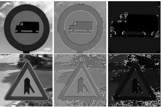
Figure 5 shows the application of line/edge and keypoint detection to traffic signs. Single- and multi-scale stabilization have eliminated many spurious key-points, one of which is shown by the small diamond of 4 pixels (zoomed image). All keypoints of the van have been detected, but three directions are still miss-ing (encircled). Here the structures have a size of 2 to 4 pixels: we are at the limit of what can be achieved by using Gabor wavelets. At the moment we are experimenting with image zooming in order to be able to work with struc-tures of smaller size. Disparity estimation is shown in Fig. 4. The stereo images were obtained by shifting left, in one image (Fig. 2 top-left) of a pair, the first

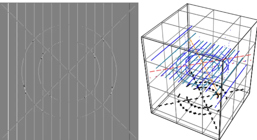
Fig. 4. Left: ledge disparity; right: 3D representation of lines, edges, depth and vertices.

vertical edge 3 pixels, the following edge 2, and the next edges 1 pixel. The second-last edge was not changed, whereas the last one was shifted right. The diagonal lines and the ring were shifted left 1 pixel. Different colors in 2D (Fig. 4 left) represent depth, which can be projected in 3D (right). There are still some problems around keypoints, and experiments with real images showed that the interval ±λ/8 of the filters that we use is too small, even of the biggest filters. The reason is that these filters are the smallest ones in the frequency domain, and a reasonable approximation of a Gaussian function requires a few samples. This problem is being solved by creating bigger filters, doing the filtering by convolution in the spatial domain.

The main conclusion is that it is now possible to create a 3D “wireframe” representation (Fig. 4 right) in which lines, edges, keypoints, vertex structure and disparity are all integrated by one extraction “process”. This will simplify 3D object recognition. The same might occur in our visual cortex, although this is still speculative. Finally, to the best of our knowledge there does not exist, also in “non-biological” work, the extraction of all attributes that we can achieve in one process, see “SUSAN” [14], “Lowe’s SIFT” [10] and e.g. [1, 15].

References

1. R. Bergevin and A. Bubel. Object-level structured contour map extraction. Comp.

Vis. and Image Underst., 91:302–334, 2003.

2. J.M.H du Buf. Responses of simple cells: events, interferences, and ambiguities.

Biol. Cybern., 68:321–333, 1993.

3. D.J. Fleet, A.D. Jepson, and M.R.M. Jenkin. Phase-based disparity measurement.

CVGIP: Image Understanding, 53(2):198–210, 1991.

4. C. Grigorescu, N. Petkov, and M.A. Westenberg. Contour detection based on nonclassical receptive field inhibition. IEEE Tr. Im. Proc., 12(7):729–739, 2003. 5. F. Heitger and et al. Simulation of neural contour mechanisms: from simple to

11. I. Ohzawa, G.C. DeAngelis, and R.D. Freeman. Encoding of binocular disparity by complex cells in the cat’s visual cortex. J. Neurophysiol., 18(77):2879–2909, 1997. 12. N. Petkov and P. Kruizinga. Computational models of visual neurons specialised in detection of periodic and aperiodic visual stimuli. Biol. Cybern., 76:83–96, 1997. 13. L.M. Santos and J.M.H du Buf. Computational cortical cell models for continuity

and texture. Biol. M. Comp. Vis. Work., Tuebingen, 2002.

14. S.M. Smith and J.M. Brady. Susan - a new approach to low level image processing.

Int. J. Comp. Vis., 23(1):45–78, 1997.

15. A. Torralba and A. Oliva. Depth estimation from image structure. IEEE Tr.

PAMI, 22(9):1226–1238, 2002.

16. J.H. van Deemter and J.M.H. du Buf. Simultaneous detection of lines and edges using compound Gabor filters. Int. J. Patt. Recogn. Artif. Intell., 14:757–777, 1996. 17. R.P. W¨urtz and T. Lourens. Corner detection in color images by multiscale

com-bination of end-stopped cortical cells. Artif. N. Net. - ICANN’97, 1997.

18. K. Yoshiyama, T. Uka, H. Tanaka, and I. Fujita. Architecture of binocular disparity processing in monkey inferior temporal cortex. Neur. Res., 48:155–167, 2004.

Fig. 5. Top: sign2 image, line/edge detection, keypoints with vertex detection after multi-scale stabilization (zoomed). Bottom: sign6.