Mass Prediction Models for Air Cargo Challenge Aircraft

(1)

UNIVERSIDADE DA BEIRA INTERIOR

Engenharia

Mass Prediction Models for Air Cargo Challenge

Aircraft

(versão corrigida após defesa)

Gustavo Lima Garcia

Dissertação para obtenção do Grau de Mestre em

Engenharia Aeronáutica

(Ciclo de estudos integrado)

Orientador: Prof. Doutor Pedro Vieira Gamboa

(2)

(3)

Abstract

The development of mass prediction models, specific for the Air Cargo Challenge competition, is presented on this dissertation. This Design/Build/Fly competition has a major interest to the University of Beira Interior, particularly to the Aerospace Sciences Department. These models are divided in two development methods: statistical and structure equations based type.

The statistical mass models are developed based on data collected from past editions and are divided in general and component based mass models. The accuracy of this type of models is, mainly, dependent on the amount of data available. On both of them three models are presented, one containing all available aircraft and two more created from the division in two groups of the original one.

Using the structure equations method, where the amount of material is determined, required to withstand the stresses that the airplane is subjected, a model is developed for each one of the three wing configurations considered, mainly CFRP, D-box CFRP and CFRP tube spar. The tail boom component equation is created independently and the remaining components masses are determined from coefficients based on geometric characteristics and the wing mass calculated. The associated average error to these models is inferior to 1%.

The results obtained from the application in the considered study cases are also presented and the respective validity, accuracy and application, in terms of design phase, for each method, are discussed.

Keywords

Mass prediction models; Air Cargo Challenge; Aircraft; UAV; Airfoil; Data fitting; Wing configuration; CFRP

(4)

(5)

Resumo

O desenvolvimento de modelos de previsão de massa para aeronaves da competição Air Cargo Challenge é apresentado nesta dissertação. Esta competição, do tipo Design/Build/Fly, tem um grande interesse para a Universidade da Beira Interior, em particular para o Departamento de Ciências Aeroespaciais. Estes modelos estão divididos em dois métodos de desenvolvimento: baseados em métodos estatísticos e em equações da estrutura

Os modelos estatísticos desenvolvidos são baseados em dados recolhidos de edições passadas e divididos em gerais e divididos por componentes. A precisão destes modelos está, essencialmente, dependente da quantidade de dados disponíveis. Em ambos, são apresentados três modelos, um contendo todas as aeronaves disponíveis e outros dois criados a partir da divisão em dois grupos do original.

Utilizando o método das equações da estrutura, é determinada onde a quantidade de material necessária, para resistir às forças a que a aeronave está sujeita, é desenvolvido um modelo para cada uma das três configurações de asa consideradas, maioritariamente em compósito de fibra de carbono, D-box em compósito de fibra de carbono e longarina em tubo de compósito de fibra de carbono. O cone da cauda é desenvolvido independentemente e a massa dos restantes componentes é determinada a partir de coeficientes baseados em características geométricas e na massa da asa calculada. O erro médio associado a estes modelos é inferior a 1%.

Apresentam-se também os resultados obtidos para a aplicação nos casos de estudo considerados e são discutidas as respetivas validade, precisão e aplicação, em termos de fase de projeto, para cada método.

Palavras-chave

Modelos de previsão de massa; Air Cargo Challenge; Aeronave; Veículo aéreo não-tripulado; Perfil alar; Ajuste de dados; Configuração de asa; Polímero de fibra de carbono reforçado

(6)

(7)

List of Figures

Figure 2.1 - UBI Airplane ACC ’07. ... 5

Figure 2.2 - UBI ACC 2003 Airplane. ... 6

Figure 2.3 - CFRP Wings. ... 7

Figure 2.4 - UBI Airplane ACC 2015 (LE and TE detail). ... 7

Figure 2.5 - AKAModell Stuttgart Airplane ACC '09 [4]. ... 8

Figure 2.6 - UBI Airplane ACC ’07 (Cargo Bay detail) [5]. ... 8

Figure 2.7 - UBI PVG ACC’ 17 (Landing Gear detail). ... 9

Figure 2.8 - University of Patras ACC ’15 (Tail detail). ... 9

Figure 3.1 - Spanwise Lift Distribution. ... 16

Figure 3.2 - Structural Validation Test. ... 16

Figure 3.3 - Simplification of the Lift. ... 17

Figure 3.4 - Single Panel Wing. ... 18

Figure 3.5 - Multiple Panels Wing. ... 19

Figure 3.6 - Carbon Fiber Configuration. ... 20

Figure 3.7 - Airfoil Divided in Two Cells. ... 21

Figure 3.8 - D-box Configuration. ... 28

Figure 3.9 - D-box Wing Section. ... 29

Figure 3.10 - Real and Approximate Airfoil Lift Distribution [1]. ... 31

Figure 3.11 - Tube Spar Configuration. ... 33

Figure 3.13 - Tail Boom [23]. ... 38

Figure 4.1 - General Mass Model. ... 45

Figure 4.2 - General Mass Model - Fixed Payloads. ... 45

Figure 4.3 - General Mass Model - Fixed Chords. ... 46

Figure 4.4 - General Mass Model - Fixed Spans. ... 46

Figure 4.5 – General Mass Model - Group I. ... 47

Figure 4.6 - General Model - Group II. ... 47

Figure 4.7 - General Mass Model - Fixed Payloads (Group I). ... 48

Figure 4.8 - General Mass Model - Fixed Payloads (Group II). ... 49

Figure 4.9 - Component Based Mass Model (Empty Mass). ... 51

Figure 4.10 - Component Based Mass Model (Total Mass). ... 51

Figure 4.11 - Component Based Mass Model - Group I (Empty Mass). ... 53

Figure 4.12 - Component Based Mass Model – Group I (Total Mass). ... 53

Figure 4.13 - Component Based Mass Model – Group II (Empty Mass). ... 54

Figure 4.14 - Component Based Mass Model – Group II (Total Mass). ... 54

Figure 4.15 - Structure Based Mass Model - Empty Mass. ... 64

(10)

(11)

List of Tables

Table 4.1 - Teams with Reports Considered. ... 43

Table 4.2 - Data Collected from the Reports. ... 44

Table 4.3 - General Mass Models Equations. ... 49

Table 4.4 - Considered Reports (Component Based Mass Models). ... 50

Table 4.5 - Component Based Mass Model Equations. ... 51

Table 4.6 - Component Based Mass Model Equations (Group I). ... 52

Table 4.7 - Component Based Mass Model Equations (Group II). ... 53

Table 4.8 - Error Comparison. ... 55

Table 4.9 - Error Comparison for Groups Division. ... 55

Table 4.10 - Coefficient of Determination Comparison. ... 56

Table 4.11 - Generic Inputs. ... 57

Table 4.12 - Specific Inputs for Carbon Fiber Configuration. ... 58

Table 4.13 - Material Properties for Carbon Fiber Configuration. ... 58

Table 4.14 - AERO@UBI_MARS Calculated and Real Masses. ... 59

Table 4.15 - AKAModell13 Calculated and Real Masses. ... 59

Table 4.16 - Specific Inputs for D-box Configuration. ... 60

Table 4.17 - Material Properties for D-box Configuration. ... 61

Table 4.18 - AERO@UBI_PVG Calculated and Real Masses. ... 61

Table 4.19 - Specific Inputs for Tube Configuration. ... 62

Table 4.20 - Material Properties for Tube Configuration. ... 62

Table 4.21 - AERO@UBI_Team Calculated and Real Masses. ... 62

Table 4.22 - Portugal Team Calculated and Real Masses. ... 63

(12)

(13)

Acronyms

ACC Air Cargo Challenge ACSYNT AirCraft SYNThesis

AIAA American Institute of Aeronautics and Astronautics APAE Portuguese Association of Aeronautics and Space CAD Computer Aided Design

CFRP Carbon Fiber Reinforced Polymer DCA Aerospace Sciences Department

FAME-W Fast and Advanced Mass Estimation Wing FEM Finite Element Method

GFRP Glass Fiber Reinforced Polymer GRG Generalized Reduced Gradient

HT Horizontal Tail

LE Leading edge

MDO Multidisciplinary Design Optimization

NASA National Aeronautics and Space Administration PDCYL Point Design of Cylindrical-bodied Aircraft

SF Safety Factor

TE Trailing edge

UBI University of Beira Interior USA United States of America

VT Vertical Tail

(14)

(15)

Nomenclature

𝐴 Area [𝑚2_] 𝑎𝑖 Variables [−] 𝐴𝑅 Aspect ratio [−] 𝑏 Span [𝑚] 𝑐 Chord [𝑚] 𝑐𝑓𝑖 Correction factors [−] 𝐶𝑑 Drag coefficient [−] 𝐶𝑖 Constants [−] 𝐶𝑙 Lift coefficient [−] 𝐶𝑚 Moment coefficient [−] 𝑑𝑠 Infinitesimal distance [𝑚] 𝑑𝜃 𝑑𝑦 Twist rate [−] 𝐸 Young’s modulus [𝑁/𝑚2_] 𝑔 Gravity acceleration [𝑚/𝑠2_] 𝐺 Shear modulus [𝑁/𝑚2_]

𝐼𝑥𝑥 Second moment of area in x axis [𝑚4]

𝐼𝑦𝑦 Second moment of area in y axis [𝑚4]

𝐽 Polar inertia moment [𝑚4_]

𝑘 Constants [−] 𝐾𝑖 Constants [−] 𝑚 Mass [𝑘𝑔] 𝑀 Moment [𝑁𝑚] 𝑛 Load factor [−] 𝑛𝑟𝑖𝑏 Number of ribs [−] 𝑝 Perimeter [𝑚] 𝑃 Concentrated load [𝑁] 𝑞 Shear flow [𝑁/𝑚] 𝑆 Wing Area [𝑚2_] 𝑆 Shear strength [𝑁]

𝑆𝑤𝑒𝑡 Wetted Surface Area [𝑚2]

𝑡 Thickness [𝑚]

𝑡

𝑐 Airfoil thickness-to-chord ratio [−]

𝑇 Torque [𝑁𝑚]

𝑉 Velocity [𝑚/𝑠]

𝑊 Weight [𝑁]

𝛥𝑦𝑖 Sum of the panels length [𝑚]

Greek Symbols

𝛽 Bending slope [𝑑𝑒𝑔𝑟𝑒𝑒]

(16)

𝜃 Rotation angle [𝑑𝑒𝑔𝑟𝑒𝑒] 𝜃 Twist angle [𝑑𝑒𝑔𝑟𝑒𝑒] 𝜆 Tapper [−] 𝜌 Density [𝑘𝑔/𝑚3_] 𝜎 Normal stress [𝑁/𝑚2_] 𝜏 Shear stress [𝑁/𝑚2_]

𝜔 Distributed load value [𝑁/𝑚]

Subscripts

A Area

box D-box

CB Cargo Bay

core Core related

empty Empty

est Estimated

face Web Face related

fus Fuselage

h, HT Horizontal Tail

i,j Counters

LG Landing Gear

material Material

max Maximum value

p Perimeter

pay Payload

R Cell Number

real Real

rib Rib related

skin Skin related spar Spar Cap related

syst Systems

tb Tail Boom

tip Wing Tip

tube Tube

VT Vertical Tail

wall Cell Wall

wing, w Wing related

(17)

1 Introduction

1.1 Motivation

The need to have a precise estimate of an airplane mass, at the early stages of aircraft design, has been proven to be crucial to maintain the capability to perform the sizing mission without increasing the take-off mass [1]. In any type of aircraft, the preliminary value obtained is essential to define and calculate the succeeding design parameters.

The Aerospace Sciences Department (DCA) of the University of Beira Interior (UBI) has a major interest in the Air Cargo Challenge (ACC) competition. Having participated in all editions until today, with three wins (two since the competition became international in 2007), it has become a very important event to improve knowledge and apply new techniques, required to develop such project.

In this competition, the experience has demonstrated the major significance of a correct estimation of the aircraft final mass. To further optimize the aircraft design, more accurate models must be developed. That leads to the possibility to dedicate more time to other tasks, increasing the manufacture quality and leading to a better final product.

1.2 Air Cargo Challenge

The ACC is a biannual competition between universities, whose main objective is the design and construction of an aircraft [2], similar to the Design/Build/Fly sponsored by the American institute of Aeronautics and Astronautics (AIAA) [3], carried out in the United States of America (USA). In addition, the development of theoretical knowledge and skills, related to design and manufacturing, and the contact between students, mainly in the aeronautics and aerospace field, is stimulated, allowing the share of knowledge and experience.

The competition was created in 2003, organized under the auspices of the APAE (Portuguese Association of Aeronautics and Space), only for Portuguese universities, and took place in Lisbon, Portugal.

In 2007, the event was internationalized, maintaining the primary objectives, allowing a greater vitalization and development of it. A new reality was introduced in this edition to encourage a major participation. In addition to the prize money awarded to the winner, the possibility to organize the next edition was offered.

Regarding the competition itself, the development and construction of a radio controlled aircraft, capable of carrying the maximum payload possible, is required. There is also a need to perform the take-off from a distance equal to or less than 60 meters, to make, at least,

(18)

one turn around the airfield and to land safely, so that the flight can be considered valid. Adding to these objectives, from the 2015 edition on, it was added the need to execute a greater number of legs (defined point passages) in a determined time gap, allying the need to carry payload with the highest velocity possible. As a result of this regulation modification, there were changes in the aircraft development.

Some parameters, such as wingspan, wing area, motor type or empty take-off mass, were imposed by the regulation. This has been modified over the years to promote the increase of the number of participants, since it is necessary to carry out a new project for each edition, approximating the results of new entries and more experienced participants. However, it should be noted that, from the observation of the results, teams with more participations, are, most likely, closer to the top of the classification. Nevertheless, positive results were obtained by most recent participations of extra-European universities, from countries like China and Brazil.

1.3 Objectives

The main scope of this dissertation is the development of mass prediction models that can be used in the design of aircraft for the ACC competition.

The integration of a more precise model in the design of the aircraft, to be used in coming competitions, might lead to better results and be adopted by other universities, increasing the contribution to the state of art of mass prediction models.

It is also intended to present alternative methods to the development of these types of models, with the objective of obtaining accurate results without the complexity of other procedures.

1.4 Dissertation Layout

The dissertation begins with an introductory chapter in which the objectives and the motivation for the accomplishment of this work are exposed. There is also an explanation regarding the ACC competition, as well as its purposes, the importance to the aerospace students and, in particular, to the university.

In the second chapter, it is presented a state of art containing the evolution of the ACC aircraft and the different types of mass prediction models, regarding its development and application.

In the third chapter, the mass models are introduced, containing the explanation concerning the implemented methods, including the equations derivation.

(19)

Then, in the fourth chapter, the results obtained for each method are presented, accompanied by an analysis, focused on the errors associated to each one and their accuracy and validity.

Finally, the conclusions, an overview of the developed work and possible recommendations for future work are presented in the fifth chapter.

(20)

(21)

2 Literature Review

2.1 State of Art

2.1.1 Air Cargo Challenge Aircraft

These aircraft are built with the main purpose of carrying the maximum payload.

Over the years, regulations have imposed limitations, mostly associated with geometry, and, in recent years, there has been a need to cover as much distance as possible within a given period of time. The existence of a more complex project was then imposed due to the need to ally the payload transport to the performance of the airplane, in order to obtain a higher score possible.

Taking that into account, there was a need to evolve from a structural point of view, combining technological advances with the ease of access to certain materials and construction techniques, thus making changes in the configuration of these aircraft.

In the first editions of the competition, the airplanes had structures made, essentially, of balsa wood and covering film, like it is possible to verify in the wing configuration in Figure 2.1, with the aim of imparting mechanical resistance and shape, respectively. There were also others made of fiber-glass and foam (see Figure 2.2). The introduction of a more extensive use of composite structures occurred in the 2007 edition, in which it was possible to observe the existence of composite carbon fiber tubes used for the tail boom (see Figure 2.1).

(22)

Figure 2.2 - UBI ACC 2003 Airplane.

Of course, due to the mechanical properties of this type of structure being more adequate to the necessities in question and to the fact that the competition has evolved, thus increasing the financial capacity of the participants, the use of composites was extended to other components of the aircraft. The main change was in the wing structure, namely the wing spar, which has become, fundamentally, a CFRP tube (see Figure 2.3 (a)), thus resisting bending and twisting strength with an obvious decrease in weight.

Another aspect to consider is the fact that some competitors have adopted more complex flaps, to which greater aerodynamic loads are associated in the wing, being necessary to increase the resistance to these forces and moments. This implied extending the use of carbon fiber composites to a greater percentage of the wing, becoming spars (see Figure 2.3 (b) (c)) and skin made of this material (see Figure 2.3 (c) (d)).

(23)

Figure 2.3 - CFRP Wings.

It is also worth noting reinforcements in the leading and trailing edges in balsa (see Figure 2.4), being used glass fiber or carbon composite in more recent aircraft.

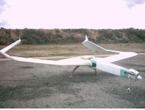
Regarding the configuration of the fuselage, it is possible to divide it into two cases: full length tube, where the cargo bay is attached (see Figure 2.5) and traditional fuselage, where the payload is placed in the cargo bay and a tail boom is used for the remaining length (see Figure 2.1).

(24)

Figure 2.5 - AKAModell Stuttgart Airplane ACC '09 [4].

The cargo bay is essentially made of balsa wood and covering film (see Figure 2.6) or, in some cases, composites. In the case of the landing gear, in the situations in which it is adopted, there are several philosophies applied in its construction, being possible to divide it in a two wheels configuration, connected by a tube (see Figure 2.7), often in CFRP, and main and secondary landing gear (see Figure 2.5). Note also the differences in the complexity of the landing gear component, with the existence of simple structures, there being cases in which this part of the aircraft is discarded, and others developed with special attention to the preservation of the integrity of the aircraft, since there is a need to avoid compromise it, that could prevent future attempts or even disqualification of the flight.

(25)

Figure 2.7 - UBI PVG ACC’ 17 (Landing Gear detail).

As for the planes’ tail surfaces, it is possible to verify that, despite the increase of composite structures, the magnitude of the forces is much lower, comparing with the wing, resulting in structures similar to those used in the beginnings of the competition, i.e., balsa wood and covering film, resulting in very reduced masses (seeFigure 2.8).

(26)

2.1.2 Mass Prediction Models

For the design of an aircraft it has been proved that an adequate weight estimate is essential, that is, that it provides values of the final mass of the aircraft that are close to reality [1]. Given this, there are many models proposed over time, usually developed for a specific type of aircraft. Dababneha and Kipouros [6] present a review of the existing methods and a division in classes. This division, based on their complexity, elaborated by Elham et al. [7], is presented next:

 Class I: In this class, the equations representing the mass are essentially developed from statistical data as functions of parameters such as empty mass, payload and fuel mass. In this situation, the initial data are scarce and, usually, only the required range and velocity are available, resulting in simple equations with a high associated error when compared to other more effective methods. Methods of this class are presented by Roskam [8], Jenkinson [9], Raymer [1] and Torenbeek [10], and Weights Analysis for Advanced Transportation Systems (WAATS), the program developed by National Aeronautics and Space Administration (NASA) [11].

 Class II: As in class I methods, these are based on statistical data. However, in this case, the designer has access to information regarding the influence that his choices, related to geometry and other aspects of the components, have on the final mass of the aircraft. Semi-empirical relationships based on essentially geometric characteristics are used, and may or may not be divided into components (fuselage, wing, tail, landing gear). Examples of these methods are presented by Torenbeek [10], Raymer [1], Niu [12], Jenkinson [9] and Howe [13].

 Class III: In this situation, physics based on structural analysis is used rather than statistical data. Usually FEM (finite element method) is used. The various components are sized based on the structural requirements and the weight is calculated based on volumes and densities of the materials to be used. Examples are the works elaborated by Bindolino [14] and Ardema et al. [15] who developed the Point Design of Cylindrical-bodied Aircraft (PDCYL) program, integrated in the AirCraft SYNThesis (ACSYNT) program developed by NASA.

 Class IV methods are also presented and described as being developed for use outside the conceptual design zone and preliminary design. They are more detailed methods, based on FEM, than the class III ones, adding to the mass calculation CAD models and components from catalogues and suppliers.

It is also presented a class II & ½, described as semi-empirical methods that use elemental analysis, based on the stiffness and mechanical resistance of the materials, combined with statistical data. The amount of material required is calculated to withstand stress using simple structure equations. Examples are the work of Burt [16], Torenbeek [17], Elham et al.

(27)

[7], FAME-W (Fast and Advanced Mass Estimation Wing) software developed by Airbus Germany [18] and Dijk [19], who created a program for Airbus Industry in Toulouse.

From the presented examples, it is possible to notice that the evolution of the computational capacity associated with the refinement of existing methods resulted in greater accuracy. Also note the existence of methods developed by authors that appear associated with design books, as well as models developed and applied by companies that use their aircraft data and then, in exchange with competitors, have access to more data, allowing more accurate results. It is also possible to perceive the difference between types of methods, both in terms of their complexity and in the way they are presented, that is, there are models from which an estimate is obtained for the total weight of the aircraft, others where it is possible to know the estimate for each constituent group and also estimate by component or set of components. There are also some examples of methods developed specifically for wing mass prediction, a critical component in any type of aircraft [15].

In the examples presented by the books focused on aircraft design, it is possible to observe the division of the models associated with each type of airplane by its application [1], [10]. It should also be noted that, for most models, the range of its applicability is specified, that is, the size limitation in terms of geometry or mass for which they have been developed and consequently for which they are valid.

(28)

(29)

3 Methodology

In this chapter, the mass models are introduced. The equations, along with the mathematical methods used, the derivations, the simplifications and the necessary considerations are presented.

3.1 Statistical Models

To determine the required equations for each model presented hereafter it is necessary to define the method adopted, based on the conducted research.

Due to the fact that the variables are independent, the equation considered adequate to represent the mass, 𝑚, has the following form:

𝑚 = 𝑘 ∏ 𝑎_𝑖𝑐𝑖

𝑛

𝑖=1

(3.1) where 𝑘 is a constant, 𝑐𝑖 are coefficients and 𝑎𝑖 are variables.

The least square fitting method minimizes the sum of square errors and the following objective function is used in order to determine the unknown coefficients:

𝑂𝑏𝑗𝑒𝑐𝑡𝑖𝑣𝑒 𝐹𝑢𝑛𝑐𝑡𝑖𝑜𝑛 = ∑(𝑚𝑒𝑠𝑡𝑗− 𝑚𝑟𝑒𝑎𝑙𝑗) 2 𝑚𝑟𝑒𝑎𝑙2 _𝑗 𝑘 𝑗=1 (3.2) where 𝑚𝑒𝑠t is the estimated mass and 𝑚𝑟𝑒𝑎𝑙 is the real mass.

The iterative process minimizes the difference between the real value for the mass and the one calculated using the defined equation, varying the coefficients in order to approximate these values. To do so, the Excel Solver is used and a nonlinear Generalized Reduced Gradient (GRG) method is applied. These methods are algorithms used to determine the solution of non-linear problems, with the main application being optimization [20].

The coefficient of determination, 𝑅2_{, is the proportion of the variance in the dependent}

variable that is predictable from the independent variable. A closer value to one means an adequate fit of the data. If the parameter takes a value near zero, the fitting does not represent the data properly [21]. The expression used to calculate the coefficient of determination is: 𝑅2_{= 1 −}∑ (𝑚𝑒𝑠𝑡𝑗− 𝑚𝑟𝑒𝑎𝑙𝑗) 2 𝑘 𝑗=1 ∑ (𝑚𝑟𝑒𝑎𝑙_𝑗− 𝑚̅̅̅̅̅̅̅)𝑟𝑒𝑎𝑙 2 𝑘 𝑗=1 (3.3) where 𝑚̅̅̅̅̅̅̅ is the mean value of real masses.

(30)

3.1.1 General Mass Model

This is a class I model, whose developed equation has the following form, where the unknown values are determined implementing the previously described process:

𝑚 = 𝑘 𝑎₁𝑐1_𝑎

2

𝑐2_𝑎

3

𝑐3 _(3.4)

where the variables 𝑎1, 𝑎2 e 𝑎3 represent the wingspan, wing chord and payload (or wing area,

aspect ratio and payload), respectively [22].

3.1.2 Component Based Mass Model

This class II model is developed considering the different constituent parts of the aircraft, namely, wing, horizontal and vertical tails, systems, landing gear, fuselage and payload. Again, the previously described method was implemented with the following equations and parameters of interest for each component.

The mass of the wing is given by:

𝑚𝑤𝑖𝑛𝑔= 𝑘𝑤𝑖𝑛𝑔𝑏 𝑐_{1𝑤𝑖𝑛𝑔} 𝑐𝑐2𝑤𝑖𝑛𝑔_𝜆𝑐3𝑤𝑖𝑛𝑔₍𝑡 𝑐) 𝑐_{4𝑤𝑖𝑛𝑔} (3.5) where the variables 𝑏, 𝑐, 𝜆 and (𝑡

𝑐) represent span, chord, taper ratio and airfoil

thickness-to-chord ratio, respectively, and the constant and the coefficients are associated to the wing mass function.

The mass of the horizontal and vertical tails is given by:

𝑚𝐻𝑇/𝑉𝑇= 𝑘𝐻𝑇/𝑉𝑇𝑏𝐻𝑇/𝑉𝑇

𝑐_{1𝐻𝑇/𝑉𝑇}

𝑐_{𝐻𝑇/𝑉𝑇}𝑐2𝐻𝑇/𝑉𝑇 (3.6)

where the variables, the constant and the coefficients represent the same parameters, but associated to the horizontal and vertical tails.

The systems, 𝑚𝑠𝑦𝑠𝑡, landing gear, 𝑚𝐿𝐺, and fuselage, 𝑚𝑓𝑢𝑠, masses are considered constant,

result of the verification that these values have small variations. The empty mass, 𝑚𝑒𝑚𝑝𝑡𝑦, is

given by:

𝑚𝑒𝑚𝑝𝑡𝑦= 𝑚𝑤𝑖𝑛𝑔+ 𝑚𝐻𝑇+ 𝑚𝑉𝑇+ 𝑚𝑓𝑢𝑠+ 𝑚𝑠𝑦𝑠𝑡+ 𝑚𝐿𝐺 (3.7)

The payload mass, 𝑚𝑝𝑎𝑦, is specified by the user. The sum of all previous parameters results

in the following expression for the final mass of the aircraft:

(31)

3.2 Structure Type Based Mass Models

These class II & ½ models are based on the equations that relate the geometric and mechanical characteristics of the components of an aircraft with the forces and moments to which it is subjected. The expressions obtained allow the determination the quantity of material, for certain expected operating conditions, necessary for the fulfilment of the imposed mission. It is then possible to get the resulting mass of each component by summing the fractions obtained to resist each force or moment, as it is explained later.

It is also important to take into account the fact that deformations, resulting from stresses, may have implications in performance and structural integrity, due to aeroelastic instability. Given that, it is considered appropriate to limit some of these structural displacements. To determine the appropriate value to use in each element, a critical analysis must be conducted.

In order to establish the allowable stress, for the material’s mechanical properties a safety factor, 𝑆𝐹, is defined.

𝑆𝐹 = 𝑢𝑙𝑡𝑖𝑚𝑎𝑡𝑒 𝑠𝑡𝑟𝑒𝑠𝑠

𝑎𝑙𝑙𝑜𝑤𝑎𝑏𝑙𝑒 𝑠𝑡𝑟𝑒𝑠𝑠 (3.9)

Due to the fact that the calculated material mass is fully necessary to withstand the loads, some mass penalty factors related to the interfaces, required to join different parts, and to extra material, needed to bond different elements, are defined, so that the final mass obtained for the wing is adjusted to be closer to the reality.

In the wing panels with taper, the root chord is considered, resulting in oversizing. However, it has been verified that the influence in the final result is not significant. For this reason, the difference is ignored, simplifying the model.

Based on the observation of the different wing structures used in the ACC aircraft, three wing structure types were considered in this study, namely, load bearing skin structure (section 3.2.3), D-box (section 3.2.4) and tube main spar (section 3.2.5).

3.2.1 Load Conditions

To size the structure it is necessary to consider the loads it is subjected to. In this study, two situations are considered: flight (see Figure 3.1) and ground test (see Figure 3.2).

(32)

Figure 3.1 - Spanwise Lift Distribution.

Figure 3.2 - Structural Validation Test.

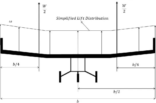
For the first case, the lift distribution is simplified as a uniformly distributed load. For the calculations, in some situations, the lift in the half span is assumed to be a concentrated load applied in its centre, in order to simplify the model (see Figure 3.3). Both the bending moment and shear force have their maximum values at the wing root decreasing to zero at the tip.

(33)

Figure 3.3 - Simplification of the Lift.

The structural validation test, required by the competition’s regulation, consists in supporting the aircraft at the wing tips and loading it. In this case, the bending moment is also maximum at the root and zero at the wing tip. However, the shear force is constant throughout the wing.

The distributed load value, 𝜔, is defined as:

𝜔 =𝑛𝑊

𝑏 (3.10)

where 𝑛 is the load factor and 𝑊 is the airplane weight.

Both these cases are considered in the sizing of the structure and the critical situation is selected.

3.2.2 Wing Panels

Due to the possible existence of tapper, the wing might be divided in panels. If the chord of the wing is constant along the span, this component can be composed by a single panel such as in Figure 3.4. In this case, the characteristics of the transversal section are defined at the root of the wing’s half-span and are constant throughout it.

(34)

Figure 3.4 - Single Panel Wing.

However, in almost all aircraft in the ACC competition, wings have tapper. This chord variation might be constant throughout the wing span or the tapper might vary. In both cases the wing is composed by panels (see Figure 3.5). The sizing is done for the first panel, with the remaining sections characteristics being determined based on the obtained for the first and some considerations regarding the impact of the respective stresses along the wing span. The sizing is done at panel’s root, so the characteristics are constant throughout the panel. It also considered the chord variation, so, to determine the required material, sections are defined at the panels’ edges.

(a) Top View

(b) Front View

(35)

Figure 3.5 - Multiple Panels Wing.

3.2.3 Load Bearing Skin Wing Configuration

For this first case, the structure thereof can be described as being predominantly manufactured in carbon fiber composite with a foam core, resulting in a sandwich configuration exemplified in Figure 3.6.

Some simplifications are assumed in the calculation of the required material to withstand each stress. It was considered that only the spar cap would resist bending loads (both for flight and ground test). The allowable stress and tip deflection are taken as limiting factors. The thickness of the spar web results from the sum of the amount of material required to withstand the shear and the torsion stresses.

(c) Half Span Deflection. (a) Top View.

(36)

Figure 3.6 – Load Bearing Skin Wing Configuration.

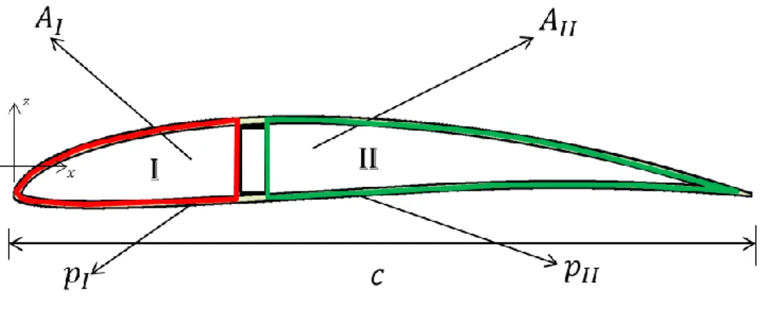
In the torsion case, being the section airfoil made of composite, it is divided into two cells having the web as a common element (see Figure 3.7). The perimeter of cell I and cell II are represented in red and green, respectively. The quantity of material required is obtained to withstand the resulting shear flow in each cell. For the sake of simplicity, the thickness of the shell is constant in both cells, thus obtaining an oversizing in the cell where the shear flow is smaller, proving that this was not problematic for the final result. Associated with the need to resist the torque, it was still considered relevant to limit the wing tip twist. The thickness considered for mass calculation is selected for the different loading cases, from the comparison of the results obtained, to the critical situation.

(37)

Figure 3.7 - Airfoil Divided in Two Cells.

The following equations are presented as the basis for the calculation and are accompanied by the deduction and some considerations to be taken into account.

The constants associated with the area are inversely proportional to the chord squared and airfoil thickness-to-chord ratio.

𝐾_𝐴𝐼= ( 𝐴𝐼 𝐴𝑎𝑖𝑟𝑓𝑜𝑖𝑙) 𝐴𝑎𝑖𝑟𝑓𝑜𝑖𝑙 𝑐2₍𝑡 𝑐) (3.11) 𝐾_𝐴𝐼𝐼= ( 𝐴𝐼𝐼 𝐴𝑎𝑖𝑟𝑓𝑜𝑖𝑙) 𝐴𝑎𝑖𝑟𝑓𝑜𝑖𝑙 𝑐2₍𝑡 𝑐) (3.12)

where 𝐴𝐼, 𝐴𝐼𝐼 and 𝐴𝑎𝑖𝑟𝑓𝑜𝑖𝑙 are the cell I, cell II and airfoil cross-section areas, respectively.

Assuming that the thickness-to-chord ratio varies only a few per cent, then the perimeter’s constants are only functions of the chord.

𝐾𝑝𝐼= ( 𝑝𝐼 𝑝𝑎𝑖𝑟𝑓𝑜𝑖𝑙) 𝑝𝑎𝑖𝑟𝑓𝑜𝑖𝑙 𝑐 (3.13) 𝐾𝑝𝐼𝐼 = ( 𝑝𝐼𝐼 𝑝𝑎𝑖𝑟𝑓𝑜𝑖𝑙) 𝑝𝑎𝑖𝑟𝑓𝑜𝑖𝑙 𝑐 (3.14)

(38)

Regarding the bending strength:

The second moment of area, 𝐼𝑥𝑥, according to the axes represented in Figure 3.7, is given by:

𝐼𝑥𝑥= ∫ 𝑧2𝑑𝐴 𝐴

(3.15) where 𝑑𝐴 is the infinitesimal area of the arbitrary shape, and 𝑧 is the distance from the x-axis to 𝑑𝐴.

Neglecting the geometry of the section and assuming that the entire transversal element area is concentrated in its centroid, the second moment of area is simplified to:

𝐼𝑥𝑥 = 𝐴𝑑2 (3.16)

where 𝐴 is the section area and 𝑑 is the distance from the x-axis to the section’s centroid. Taking into account that,

𝐴 = 2𝐴𝑠𝑝𝑎𝑟 (3.17)

𝑑 = (𝑐 ( 𝑡 𝑐)

2 ) (3.18)

where 𝐴𝑠𝑝𝑎𝑟 is the spar cap area and substituting Eq. (3.17) and Eq. (3.18) into Eq. (3.16), the

expression for the second moment of area is:

𝐼𝑥𝑥 =

𝐴𝑠𝑝𝑎𝑟𝑐2(𝑡_𝑐) 2

2

(3.19)

For the calculation of the required spar cap area, the limiting criteria are the bending moment and the tip deflection. For the flight, it is assumed the simplification described in the previous section where the lift in the half-span is replaced by a concentrated load.

Starting with the known equations for normal stress, 𝜎𝑦, and bending moment, 𝑀𝑥, from the

axes represented Figure 3.6:

𝜎𝑦= 𝑀𝑥𝑐 ( 𝑡 𝑐) 2 𝐼𝑥𝑥 (3.20)

(39)

𝑀𝑥=

𝑛𝑊𝑏

8 (3.21)

Substituting Eq. (3.19) and Eq. (3.21) into Eq.(3.20), the spar cap area is determined as follows: 𝐴𝑠𝑝𝑎𝑟 𝑀𝑓𝑙 = 1 8𝜎_{𝑦𝑚𝑎𝑥} 𝑛𝑊𝑏 𝑐 (_𝑐𝑡) (3.22)

where 𝜎_{𝑦𝑚𝑎𝑥} is the maximum allowable normal stress.

Due to the simplification considered for the lift distribution, the bending moment varies with the span squared. Once verified that, the spar cap area is also considered to vary with the span squared, for the remaining panels, and it is determined using the following expression:

𝐴𝑠𝑝𝑎𝑟_𝑖 = (

𝑏 − Δ𝑦𝑖

𝑏 )

2

𝐴_{𝑠𝑝𝑎𝑟1} (3.23)

where Δ𝑦𝑖 is the sum of the panels’ length until the respective position.

In case of the ground test, the load factor is eliminated from Eq. (3.21) and it is considered that the force is applied at the wing tip, resulting on the following bending moment:

𝑀𝑥=

𝑊𝑏

4 (3.24)

and substituting Eq. (3.24) and Eq. (3.19) into Eq. (3.20), the required spar cap area is given by: 𝐴𝑠𝑝𝑎𝑟 𝑀𝑔𝑡 = 1 4𝜎_{𝑦𝑚𝑎𝑥} 𝑊𝑏 𝑐 (_𝑐𝑡) (3.25)

In the deflection case, considering that the wing bending curvature occurs mainly close to the root, the expression of the tip deflection, 𝛿𝑡𝑖𝑝, is given as (the parameters are represented in

Figure 3.5):

𝛿𝑡𝑖𝑝= 𝛿1+ 𝛽1

𝑏 − Δ𝑦1

2 + 𝛿2 (3.26)

where, 𝛿1 is the deflection at the first panel tip, 𝛽1 is the bending slope at the first panel tip

(40)

That said, the expressions for the respective parameters are considered, according to the axes represented in Figure 3.5:

𝛽 = 𝜔𝐿 3 6𝐸𝐼𝑥𝑥 +𝑀𝑥𝐿 𝐸𝐼𝑥𝑥 (3.27) 𝛿 = 𝜔𝐿 4 8𝐸𝐼𝑥𝑥 +𝑀𝑥𝐿 2 2𝐸𝐼𝑥𝑥 (3.28)

where 𝛽 is the bending slope, 𝛿 is the deflection, 𝐿 is the panel length and 𝐸 is the Young’s modulus.

Assuming that the spar cap area decrease is proportional to the span squared, the second moment of area for the remaining wing is assumed to be:

𝐼_𝑥𝑥2= (𝑏 − Δ𝑦𝑖 𝑏 )

2

𝐼_𝑥𝑥1 (3.29)

Initially, the panel length and the moment, resulting from the distributed load for the remaining wing, have to be defined:

𝐿 =Δ𝑦1 2 (3.30) 𝑀 =𝑛𝑊 𝑏 ( 𝑏 − Δ𝑦1 4 ) ( 𝑏 − Δ𝑦1 2 ) (3.31)

Knowing the necessary data, substituting Eq. (3.26), Eq. (3.29), Eq. (3.30) and Eq. (3.31) into Eq. (3.28), the expression for the deflection is obtained and, rearranging it, the required spar cap area is determined:

𝛿𝑡𝑖𝑝= 𝑛𝑊 192𝐸𝑏𝐴𝑠𝑝𝑎𝑟𝑐2( 𝑡 𝑐) 2(3𝑏4− 3𝑏2Δ𝑦12+ 𝑏Δ𝑦13+ 2Δ𝑦14) (3.32) 𝐴𝑠𝑝𝑎𝑟𝛿 = 1 192𝐸𝛿𝑡𝑖𝑝 𝑛𝑊 𝑏𝑐2₍𝑡 𝑐) 2(3𝑏 4_{− 3𝑏}2_Δ𝑦 12+ 𝑏Δ𝑦13+ 2Δ𝑦14) _(3.33)

(41)

The remaining panels’ spar cap area is determined using Eq. (3.23).

The final spar cap area is the maximum value between the ones calculated for the bending moment (flight, Eq. (3.22), and ground test, Eq. (3.25)) and for the maximum allowable wing tip deflection, Eq. (3.33), and is given by the following expression:

𝐴𝑠𝑝𝑎𝑟= max(𝐴𝑠𝑝𝑎𝑟 𝑀𝑓𝑙

; 𝐴𝑠𝑝𝑎𝑟 𝑀𝑔𝑡

; 𝐴𝑠𝑝𝑎𝑟𝛿 ) (3.34)

In the shear stress case, 𝜏, its maximum value (located in the neutral axis) is calculated using the following expressions:

𝜏 =3 2 𝑆𝑧 2𝑡𝑓𝑎𝑐𝑒𝑐 ( 𝑡 𝑐) (3.35) 𝑆𝑧= 𝑛𝑊 2 (3.36) 𝜏 = 3𝑛𝑊 8𝑡𝑓𝑎𝑐𝑒𝑐 ( 𝑡 𝑐) (3.37)

where 𝑆𝑧 is the maximum shear force and 𝑡𝑓𝑎𝑐𝑒 is the web face thickness.

Hereupon, the thickness expression is determined from Eq. (3.37):

𝑡_{𝑓𝑎𝑐𝑒}𝑓𝑙 = 3 8𝜏𝑚𝑎𝑥

𝑛𝑊

𝑐 (_𝑐𝑡) (3.38)

where 𝜏𝑚𝑎𝑥 is the maximum allowable shear stress.

For the ground test, the load factor is not considered in Eq. (3.38), resulting in:

𝑡_{𝑓𝑎𝑐𝑒}𝑔𝑡 = 3 8𝜏𝑚𝑎𝑥

𝑊

𝑐 (_𝑐𝑡) (3.39)

As already was mentioned, on the ground test, the force is constant throughout the wing and, in flight, its value is maximum at the root and null at the tip.

(42)

In the torsion case, the division of the airfoil into two cells is considered, with the following expressions being implemented for torque, 𝑇, and twist rate, 𝑑𝜃

𝑑𝑦: 𝑇 = ∑ 2𝐴𝑅𝑞𝑟 𝑛 𝑅=1 (3.40) 𝑑𝜃 𝑑𝑦= 1 2𝐴𝑅𝐺 ∮ 𝑞𝑅 𝑑𝑠 𝑡 (3.41)

where 𝐴𝑅 and 𝑞𝑅 are the area and shear flow of the 𝑅𝑡ℎ cell, 𝐺 is the shear modulus, 𝑑𝑠 is the

infinitesimal distance along the cell wall and 𝑡 is the cell wall thickness. Based on that, a three equations system is defined:

{ (𝑑𝜃 𝑑𝑦)_𝐼 = 1 2𝐴𝐼𝐺 (𝑞𝐼 𝑝𝐼 𝑡 − 𝑞𝐼𝐼 𝑐 (𝑡_𝑐) 𝑡 ) (𝑑𝜃 𝑑𝑦)_𝐼𝐼= 1 2𝐴𝐼𝐼𝐺 (−𝑞𝐼 𝑐 (𝑡_𝑐) 𝑡 + 𝑞𝐼𝐼 𝑝𝐼𝐼 𝑡 ) 𝑇 = 2𝐴𝐼𝑞𝐼+ 2𝐴𝐼𝐼𝑞𝐼𝐼 (3.42) (3.43) (3.44)

where 𝑞𝐼 and 𝑞𝐼𝐼 are shear flows in cell I and II, respectively.

The unknowns are the two shear flows in the cells and the thickness required to ensure the determined twist at the wing tip.

In order to solve the system and based on the known values, the following parameters are defined: 𝑡 = 2𝑡𝑠𝑘𝑖𝑛 (3.45) 𝑇 =1 2𝜌𝑉 2𝑏 2 𝑐 2_𝐶 𝑚 (3.46) 𝑞𝐼= 𝑞𝐼𝐼𝐶1 (3.47) 𝐶1= 𝐾𝑝𝐼𝐼+ 𝐾𝐴𝐼𝐼 𝐾𝐴_𝐼 ( 𝑡 𝑐) 𝐾𝐴𝐼𝐼𝐾𝑝𝐼 𝐾 + ( 𝑡 𝑐) (3.48)

(43)

𝐶2=

𝜌𝑉2_𝑏𝐶 𝑚

8 (_𝑐𝑡) (3.49)

𝑞 = 𝑡𝜏 (3.50)

where 𝑡𝑠𝑘𝑖𝑛 is the skin face thickness, 𝜌 is the air density, 𝑉 is the velocity, 𝐶𝑚 is the

coefficient of pitching moment and 𝐶1 and 𝐶2 are constants.

Once Eq. (3.45) to Eq. (3.50) are substituted in the three equations system and this one is solved, the expressions for the shear flows are known and thicknesses are also determined to withstand the torque. The thicknesses expressions obtained are (torque, in cell I and II, and twist): 𝑡𝑠𝑘𝑖𝑛𝐼= 𝐶2 (𝐾𝐴_𝐼𝐼+ 𝐾𝐴_𝐼𝐶1)2𝜏𝑚𝑎𝑥 (3.51) 𝑡𝑠𝑘𝑖𝑛𝐼𝐼= 𝐶1𝐶2 (𝐾𝐴_𝐼𝐼+ 𝐾𝐴_𝐼𝐶1)2𝜏𝑚𝑎𝑥 (3.52) 𝑡𝑠𝑘𝑖𝑛𝜃 = 𝐶2(𝐶1𝐾𝑝𝐼− ( 𝑡 𝑐)) 𝑏 (8𝐾𝐴𝐼𝑐 ( 𝑡 𝑐) 𝐺𝜃𝑚𝑎𝑥) (𝐾𝐴𝐼𝐼+ 𝐾𝐴𝐼𝐶1) (3.53)

where 𝜃𝑚𝑎𝑥 is the maximum allowable wing tip twist angle.

The final skin thickness is the maximum value between the ones determined to withstand the torque (cell I, Eq. (3.51), and cell II, Eq. (3.52)) and to guarantee the allowable wing tip twist, Eq. (3.53), and is given by the following expression:

𝑡𝑠𝑘𝑖𝑛= max(𝑡_{𝑠𝑘𝑖𝑛𝐼}; 𝑡_{𝑠𝑘𝑖𝑛𝐼𝐼}; 𝑡𝑠𝑘𝑖𝑛𝜃 ) (3.54)

The final web face thickness is the sum of the maximum value, required to withstand the shear stress, between the ones calculated for flight, Eq. (3.38), and ground test, Eq. (3.39), and the thickness required to withstand the torsion, obtained in Eq. (3.54). The web face thickness is given by the following expression:

𝑡𝑓𝑎𝑐𝑒= max( 𝑡𝑓𝑎𝑐𝑒 𝑓𝑙

(44)

The wing mass might be determined from user-defined data, allowing realistic values for the construction, rather than the thicknesses obtained from the expressions, which might not be suitable from the practical perspective.

The core foam mass, 𝑚𝑐𝑜𝑟𝑒, is determined from a thickness value deemed suitable by the

user.

𝑚𝑐𝑜𝑟𝑒= 𝑡𝑐𝑜𝑟𝑒𝑏 (𝑝𝑎𝑖𝑟𝑓𝑜𝑖𝑙+

𝑡

𝑐𝑐) 𝜌𝑐𝑜𝑟𝑒

(3.56)

where 𝑡𝑐𝑜𝑟𝑒 is the core thickness and 𝜌𝑐𝑜𝑟𝑒 is the foam density.

3.2.4 D-box Wing Configuration

The second configuration consists of a D-box structure, from the leading edge until the spar. As before, a sandwich structure is used, made of carbon fiber composite shell and foam core, simplified in Figure 3.8.

The rear section of the airfoil has ribs for the purpose of transmitting stresses to the spar and to guarantee the airfoil shape, provided by the covering film, and reinforcement in the trailing edge made of balsa wood.

(45)

Similarly to the previous case, it is considered that the bending moment is resisted by the spar caps and the shear stress by the spar web. Thus, the equations presented above are also valid.

In this case, only the D-box resists to torque, being necessary the implementation of new equations. The side view is represented in Figure 3.9, where the D-box perimeter is represented in red.

Figure 3.9 - D-box Wing Section.

The constants associated to the perimeter, 𝐾𝑏𝑜𝑥, and area, 𝐾𝑏𝑜𝑥₂, are:

𝐾𝑏𝑜𝑥= ( 𝑝𝑏𝑜𝑥 𝑝𝑎𝑖𝑟𝑓𝑜𝑖𝑙) 𝑝𝑎𝑖𝑟𝑓𝑜𝑖𝑙 𝑐 (3.57) 𝐾𝑏𝑜𝑥2= ( 𝐴𝑏𝑜𝑥 𝐴𝑎𝑖𝑟𝑓𝑜𝑖𝑙) 𝐴𝑎𝑖𝑟𝑓𝑜𝑖𝑙 𝑐2₍𝑡 𝑐) (3.58)

where 𝑝𝑏𝑜𝑥 and 𝐴𝑏𝑜𝑥 are the D-box perimeter and cross-section area, respectively.

Again, there is a need for the structure to withstand the torque and a limitation for the tip wing twist is imposed. Initially, the following expressions are used:

𝑇 = 2𝐴𝑞 (3.59)

𝑡 = 2𝑡𝑓𝑎𝑐𝑒 (3.60)

Therefore, Eq. (3.46) (resulting torque from the aerodynamic load in half span), Eq. (3.50) (resulting shear flow in a section with a given thickness and subjected to shear stress) and Eq.

(46)

(3.60) are substituted into Eq. (3.59) resulting in the following expression for the spar web thickness, required to resist to the torsion:

𝑡𝑓𝑎𝑐𝑒𝑇 =

𝜌𝑎𝑖𝑟𝐶𝑚

16𝐾𝑏𝑜𝑥𝜏𝑚𝑎𝑥

𝑉2_𝑏

(_𝑐𝑡) (3.61)

For the twist case, according to the axes represented in Figure 3.8, the expressions for torsion in a single cell and Eq. (3.46) (resulting torque from the aerodynamic load in half span) are considered:

𝑑𝜃 𝑑𝑦= 𝑇 𝐺𝐽 (3.62) 𝐺𝐽 =4𝐴𝑏𝑜𝑥 2 ∮𝑑𝑠_𝐺𝑡 (3.63) 𝑑𝜃 𝑑𝑦= 𝜌𝑉2_𝑏𝐶 𝑚𝐾𝑏𝑜𝑥 32𝐺𝐾_𝑏𝑜𝑥2 ₂_{𝑐 (}𝑡 𝑐) 2 𝑡𝑓𝑎𝑐𝑒 (3.64)

The required thickness is obtained from the simplification of Eq. (3.64), resulting in the following expression: 𝑡𝑓𝑎𝑐𝑒𝜃 = 𝜌𝐶𝑚𝐾𝑏𝑜𝑥 64𝐺𝐾_𝑏𝑜𝑥2 ₂_𝜃 𝑚𝑎𝑥 𝑉2_𝑏2 𝑐 (_𝑐𝑡) 2 (3.65)

The final face thickness is the maximum value between the ones determined to withstand the torque, Eq. (3.61), and to guarantee the allowable wing tip twist, Eq. (3.65), and is given by the following expression:

𝑡𝑓𝑎𝑐𝑒= max( 𝑡𝑓𝑎𝑐𝑒𝑇 ; 𝑡𝑓𝑎𝑐𝑒𝜃 ) (3.66)

It is also needed to ensure that the ribs transmit the stresses and do not fail, being necessary the sizing that allows that this component resists the shear force in the rear region of the wing. The defined constants for the ribs are:

𝐾𝑟𝑖𝑏 = ( 𝐴𝑟𝑖𝑏 𝐴𝑎𝑖𝑟𝑓𝑜𝑖𝑙) 𝐴𝑎𝑖𝑟𝑓𝑜𝑖𝑙 𝑐2₍𝑡 𝑐) (3.67)

(47)

𝐾𝑟𝑖𝑏2 =

𝑙𝑟𝑖𝑏

𝑐 (3.68)

where 𝐴𝑟𝑖𝑏 is the area and 𝑙𝑟𝑖𝑏 is the length of the rib.

Initially, the following lift simplified distribution along the chord, represented in Figure 3.10, is considered, from which the respective load is determined:

Figure 3.10 - Real and Approximate Airfoil Lift Distribution [1].

Based on to the axes represented in Figure 3.9 and from the integration of the lift along the cord it is possible to determine the load distribution value, 𝜔:

𝐿 = 2 ∫ ∫ 𝑝(𝑥) 𝑑𝑥 𝑑𝑧 𝑐 0 𝑏 2 0 (3.69) 𝑛𝑊 = 2𝑏 2∫ 𝑝(𝑥) 𝑑𝑥 𝑐 0 (3.70) ∫ 𝑝(𝑥) 𝑑𝑥 𝑐 0 = 0,15𝑐𝜔 +0,85𝑐𝜔 2 (3.71) 𝜔 =40 23 𝑛𝑊 𝑏𝑐 (3.72)

Based on that, the maximum shear force, 𝑆𝑧′, located in the spar region is determined by

integrating the distributed load from the trailing edge to the spar, resulting in the total force applied in the rib region, resulting in the following equation:

(48)

𝑆𝑧′= 𝑙𝑟𝑖𝑏 𝑙𝑟𝑖𝑏 0,85𝑐𝜔 2 (3.73)

Substituting Eq. (3.68) and Eq. (3.72) into Eq. (3.73), the shear force is simplified.

𝑆𝑧′=

400 391

𝐾𝑟𝑖𝑏2 ₂𝑛𝑊

𝑏 (3.74)

The shear stress expression is:

𝜏 =3 2 𝑆𝑧′/𝑛𝑟𝑖𝑏 𝑡𝑟𝑖𝑏𝑐 ( 𝑡 𝑐) (3.75) where 𝑛𝑟𝑖𝑏 is the number of ribs.

Finally, the product of the ribs thickness by its total number is obtained from the substitution of Eq. (3.74) into Eq. (3.75):

𝑡𝑟𝑖𝑏𝑛𝑟𝑖𝑏= 600 391 𝐾𝑟𝑖𝑏2 ₂ 𝜏𝑚𝑎𝑥 𝑛𝑊 𝑐𝑏 (_𝑐𝑡) (3.76)

The mass of the trailing edge, 𝑚𝑇𝐸, is given by:

𝑚𝑇𝐸 = 𝐾𝑇𝐸𝑐2(

𝑡

𝑐) 𝑏𝜌𝑏𝑎𝑙𝑠𝑎 (3.77)

where 𝜌𝑏𝑎𝑙𝑠𝑎 is the balsa density and the trailing edge coefficient, 𝐾𝑇𝐸, is calculated as

follows: 𝐾𝑇𝐸 = ( 𝐴𝑇𝐸 𝐴𝑎𝑖𝑟𝑓𝑜𝑖𝑙) 𝐴𝑎𝑖𝑟𝑓𝑜𝑖𝑙 𝑐2₍𝑡 𝑐) (3.78)

where 𝐴𝑇𝐸 is the trailing edge side area.

(49)

The core foam mass is determined from a thickness value deemed suitable by the user. 𝑚𝑐𝑜𝑟𝑒= 𝑡𝑐𝑜𝑟𝑒𝑏 𝑝𝑏𝑜𝑥 𝜌𝑐𝑜𝑟𝑒 (3.79)

The final mass might be determined using specified values for spar cap and web thicknesses, as previously.

3.2.5 Tube Spar Wing Configuration

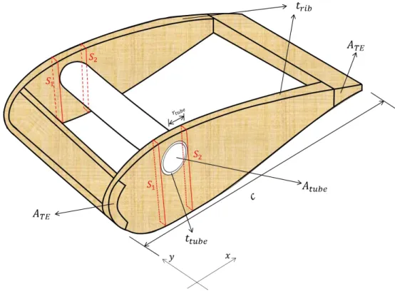
In this last configuration, illustrated in Figure 3.11., the wing is composed by a circular thin-walled section spar, with ribs to transmit the stresses and support the covering film, to provide the desired airfoil shape, with reinforcements in the leading and trailing edges made of balsa wood.

Figure 3.11 - Tube Spar Wing Configuration.

Instead of the presented so far, where the loads were divided by the different wing parts, in this situation, the required tube thickness is calculated to resist bending, shear and torsion, being, the final result, the sum of all individual thicknesses obtained for the above mentioned stresses.

For the necessary calculations, the following constant is determined from known data:

𝐾𝑡𝑢𝑏𝑒 =

𝑟𝑡𝑢𝑏𝑒

(50)

where 𝑟𝑡𝑢𝑏𝑒 is the tube radius.

The second moment of area is given by the following simplified expression for thin tubes:

𝐼𝑥𝑥 = 𝜋𝑟𝑡𝑢𝑏𝑒3 𝑡𝑡𝑢𝑏𝑒 (3.81)

where 𝑡𝑡𝑢𝑏𝑒 is the tube thickness.

As previously, the same simplification on the lift is assumed for the calculation of the bending moment. The required thickness is determined by the critical case when comparing the results for the bending moment (in flight and ground test) and the tip deflection.

Initially, based on the axes represented in Figure 3.11, the following expression is considered to determine the normal stress:

𝜎𝑦=

𝑀𝑥𝑟𝑡𝑢𝑏𝑒

𝐼𝑥𝑥

(3.82) Substituting Eq. (3.21) (bending moment), Eq. (3.81) and Eq. (3.80) into Eq. (3.82), the required tube thickness is given by the following expression:

𝑡_{𝑡𝑢𝑏𝑒}𝑀𝑓𝑙 = 1 8𝜋𝐾_{𝑡𝑢𝑏𝑒}2 _𝜎

𝑦𝑚𝑎𝑥

𝑛𝑊𝑏

𝑐2 (3.83)

For the ground test, the same process is implemented with the difference that Eq. (3.24) (bending moment with concentrated load applied on the wing tip) is considered instead of Eq. (3.21), for the bending moment determination, resulting in:

𝑡_{𝑡𝑢𝑏𝑒}𝑀𝑔𝑡 = 1 4𝜋𝐾_{𝑡𝑢𝑏𝑒}2 _𝜎 𝑦𝑚𝑎𝑥 𝑊𝑏 𝑐2₍𝑡 𝑐) 2 (3.84)

The thicknesses for the remaining sections are determined based on the assumption that it varies with the span squared:

𝑡_{𝑡𝑢𝑏𝑒𝑖}= (𝑏 − Δ𝑦𝑖

𝑏 )

2

𝑡_{𝑡𝑢𝑏𝑒1} (3.85)

In the deflection case, assuming that thickness varies with the span squared and considering Eq. (3.27) to Eq. (3.31) (deflection simplifications) and Eq. (3.81) and substituting into Eq. (3.26), the following expression for the tip deflection is obtained:

(51)

𝛿𝑡𝑖𝑝= 𝑛𝑊 192𝐸𝑏𝜋𝑟_{𝑡𝑢𝑏𝑒}3 _𝑡 𝑡𝑢𝑏𝑒 (2𝑏4_{+ 4𝑏}3_Δ𝑦 1− 15Δ𝑦12+ 14𝑏Δ𝑦13− 3Δ𝑦14) (3.86)

Rearranging Eq. (3.86), the required tube thickness is given by:

𝑡𝑡𝑢𝑏𝑒𝛿 = 1 192𝐸𝜋𝛿𝑡𝑖𝑝 𝑛𝑊 𝑏𝑟𝑡𝑢𝑏𝑒3 (2𝑏4_{+ 4𝑏}3_Δ𝑦 1− 15Δ𝑦12+ 14𝑏Δ𝑦13− 3Δ𝑦14) (3.87)

As before, the thicknesses for the remaining sections are determined, based on the assumption that it varies with the span squared, from Eq. (3.81).

The expression for the shear stress is similar to the one obtained for the previous configurations, having an obvious change in the form of tube section area, 𝐴𝑡𝑢𝑏𝑒:

𝐴𝑡𝑢𝑏𝑒= 2𝜋𝑟𝑡𝑢𝑏𝑒𝑡𝑡𝑢𝑏𝑒 (3.88) 𝜏 =3 2 𝑆𝑧 𝐴𝑡𝑢𝑏𝑒 (3.89)

Substituting the expression for the shear force, Eq. (3.36), into Eq. (3.89), the shear stress results in:

𝜏 = 3𝑛𝑊

8𝜋𝐾𝑡𝑢𝑏𝑒𝑐𝑡𝑡𝑢𝑏𝑒 (3.90)

Rearranging Eq. (3.90) the required tube thickness is:

𝑡_{𝑡𝑢𝑏𝑒}𝜏𝑓𝑙 = 3 8𝜋𝐾𝑡𝑢𝑏𝑒𝜏𝑚𝑎𝑥

𝑛𝑊

𝑐 (3.91)

For the ground test, once again, the load factor is removed from Eq. (3.91):

𝑡_{𝑡𝑢𝑏𝑒}𝜏𝑔𝑡 = 3 8𝜋𝐾𝑡𝑢𝑏𝑒𝜏𝑚𝑎𝑥

𝑊

𝑐 (3.92)

As before, for flight, the shear stress is maximum at the root and null at the tip. On the ground it is constant along the wingspan.

(52)

Regarding the torsion load bearing structure:

The circle area of the tube is given by the following equation:

𝐴 = 𝜋𝑟𝑡𝑢𝑏𝑒2 (3.93)

The expressions used for the torque and shear flow are identical to those of the D-box, Eq. (3.46) (torque resulting from the aerodynamic load in half span), Eq. (3.59) (torque resulting from the shear flow) and Eq. (3.50) (shear flow), with Eq. (3.93) being used for the area, resulting in the required thickness to withstand the torque:

𝑡𝑡𝑢𝑏𝑒𝑇 =

𝜌𝐶𝑚

8𝜋𝐾_{𝑡𝑢𝑏𝑒}2 _𝜏 𝑚𝑎𝑥

𝑉2_𝑏 _(3.94)

For the twist case, once again, the difference is the area calculation, determined from Eq. (3.93), being used Eq. (3.62) to determine the twist ratio and Eq. (3.46) to determine the torque, resulting in these expressions:

𝐺𝐽 = 2𝜋𝐾𝑡𝑢𝑏𝑒3 𝑐3𝐺𝑡𝑡𝑢𝑏𝑒 (3.95) 𝑑𝜃 𝑑𝑦= 𝜌𝑉2_𝑏𝐶 𝑚 8𝜋𝐺𝐾𝑡𝑢𝑏𝑒3 𝑐𝑡𝑢𝑏𝑒 (3.96)

From Eq. (3.96), the required tube thickness is obtained:

𝑡𝑡𝑢𝑏𝑒𝜃 =

𝜌𝐶𝑚

8𝜋𝐺𝐾𝑡𝑢𝑏𝑒3 𝜃𝑚𝑎𝑥

𝑉2_𝑏2

𝑐 (3.97)

The final tube thickness results from the sum of all individual thicknesses, required to withstand the bending moment (Eq. (3.83), Eq. (3.84) and Eq. (3.87)), the shear stress (Eq. (3.91) and Eq. (3.92)) and the torsion (Eq. (3.94) and Eq. (3.97)). For each stress, the maximum value, among the ones calculated for each limiting criteria, is considered. The expression for the tube thickness is:

𝑡𝑡𝑢𝑏𝑒 = max(𝑡𝑡𝑢𝑏𝑒 𝑀𝑓𝑙

; 𝑡_{𝑡𝑢𝑏𝑒}𝑀𝑔𝑡; 𝑡𝑡𝑢𝑏𝑒𝛿 ) + max(𝑡𝑡𝑢𝑏𝑒 𝜏𝑓𝑙

(53)

This value might be indicated by the user in order to ensure a viable value from which the mass of the component is determined.

Once again, sizing the ribs is required. In this situation, it has been determined that the maximum shear is located in positions 𝑆1 and 𝑆2, indicated in Figure 3.11.

The following calculations demonstrate the shear in those positions, assuming that spar is located at 30% of the chord.

𝑆1= 0,15𝑐𝜔 + 𝜔 +_0,85𝑐0,7𝑐 𝜔 2 0,15𝑐 ≈ 0,3𝜔𝑐 𝑆2= 0,7𝑐_0,85𝑐0,7𝑐 𝜔 2 ≈ 0,3𝜔𝑐

Based on that, it is possible to assume that the shear force value is, approximately, identical in positions 𝑆1 and 𝑆2. The shear force is then simplified such as determined in the previous

demonstrations:

𝑆𝑧′= 0,3𝜔𝑐 (3.99)

Using the equation determined in the previous section, for the distributed load, Eq. (3.72) and considering Eq. (3.99) for the shear force, substituting into Eq. (3.75), the shear stress is obtained. Rearranging the resulting equation, the product of the rib thickness by the total number of ribs is determined:

𝑡𝑟𝑖𝑏𝑛𝑟𝑖𝑏 =

36 23𝜏𝑥𝑦𝑚𝑎𝑥

𝑛𝑊

𝑐 (_𝑐𝑡) 𝑏 (3.100)

The leading and trailing edges masses are determined as follows:

𝑚𝐿𝐸/𝑇𝐸= 𝐾𝐿𝐸/𝑇𝐸𝑐2(

𝑡

𝑐) 𝑏𝜌𝑏𝑎𝑙𝑠𝑎 (3.101)

and the respective coefficients are:

𝐾𝑇𝐸= (_𝐴𝐴𝑇𝐸 𝑎𝑖𝑟𝑓𝑜𝑖𝑙) 𝐴𝑎𝑖𝑟𝑓𝑜𝑖𝑙 𝑐2₍𝑡 𝑐) (3.102)

(54)

𝐾𝐿𝐸 = ( 𝐴𝐿𝐸 𝐴𝑎𝑖𝑟𝑓𝑜𝑖𝑙) 𝐴𝑎𝑖𝑟𝑓𝑜𝑖𝑙 𝑐2₍𝑡 𝑐) (3.103) where 𝐴𝐿𝐸 is the leading edge area.

3.2.6 Tail Boom Tube

This component is used to connect the tail to the remaining airplane and provide the required length between the wing and the tail and, subsequently, the necessary stability. It is made of CFRP and it is attached to the cargo bay or the rest of the fuselage that supports the wing, as previously described. An example of the first case can be observed in Figure 3.12.

Figure 3.12 - Tail Boom [23].

The determination of the tail boom mass is independent of the wing configuration. For this component it is considered that it is necessary to resist the load applied at the tail and the need to have a limitation on the tail rotation. Based on that, it is necessary to calculate the lift force on the horizontal tail and the resulting bending moment. To do so, the following constants are determined:

𝐾ℎ = (𝑙ℎ 𝑏) 𝑏 𝑐 (3.104) 𝐾𝑡𝑏= (𝑙𝑡𝑏 𝑏) 𝑏 (3.105)

(55)

where 𝑙ℎ is the arm between the wing and horizontal tail aerodynamic centers and 𝑙𝑡𝑏 is the

tail boom length.

The horizontal tail lift is obtained from known data. That is done based on the need to balance the wing pitching moment with the horizontal tail moment, resulting in the following expressions: 𝑇 = 𝑙ℎ𝐿ℎ (3.106) 𝑇 =1 2𝜌𝑉 2_𝑏𝑐2_𝐶 𝑚 (3.107) 𝐿ℎ = 1 2𝜌𝑉 2_𝑆 ℎ𝐶𝐿_ℎ (3.108) 𝐶𝐿ℎ= 𝑏𝑐𝐶𝑚 𝑆ℎ𝐾ℎ (3.109) where 𝐿ℎ is the lift, 𝑆ℎ is the area, 𝐶𝐿_ℎ is the lift coefficient, all related to the horizontal tail.

The resulting bending moment and normal stress are determined once the lift is calculated, from Eq. (3.108). The second moment of area expression, based on the axes represented in Figure 3.12, considered is the one simplified for thin tubes.

𝑀𝑦= 𝐿ℎ𝑙𝑡𝑏 (3.110) 𝐼𝑦𝑦 = 𝜋𝑟𝑡𝑏3𝑡𝑡𝑏 (3.111) 𝜎𝑥 = 𝑀𝑦𝑙𝑡𝑏 𝐼𝑦𝑦 (3.112) where 𝑟𝑡𝑏 is the tail boom radius and 𝑡𝑡𝑏 is the tail boom tube wall thickness.

The required tail boom thickness, 𝑡𝑡𝑏, is obtained after the resulting bending moment is

determined, substituting Eq. (3.110) and Eq. (3.111) into Eq. (3.112), and based on the tube radius defined:

𝑡𝑡𝑏𝑀 =

𝜌𝐶𝑚𝐾𝑡𝑏

2𝐾ℎ𝜋𝑟𝑡𝑏2𝜎𝑥𝑚𝑎𝑥

𝑏𝑐2_𝑉2 _(3.113)

(56)

𝜃 = 𝐿ℎ𝑙𝑡𝑏

2

2𝐸𝐼𝑦𝑦

(3.114)

Substituting Eq. (3.104) and Eq. (3.109) into Eq. (3.113), the lift in the horizontal tail is:

𝐿ℎ =

𝜌𝑉2_𝑐𝑏𝐶 𝑚

2𝐾ℎ

(3.115)

Substituting Eq. (3.109), Eq. (3.115) and Eq. (3.111) into Eq. (3.114), the rotation is given as:

𝜃 =𝜌𝑉

2_𝑐𝑏𝐶

𝑚𝑙𝑡𝑏2

4𝐾ℎ𝐸𝜋𝑟𝑡𝑏3𝑡𝑡𝑏

(3.116)

The required tail boom thickness is determined from rearranging Eq. (3.116), resulting in the following expression:

𝑡𝑡𝑏𝜃 =

𝜌𝐶𝑚𝐾𝑡𝑏2

4𝜋𝐸𝑟𝑡𝑏3𝐾ℎ𝜃𝑚𝑎𝑥

𝑐3_𝑏𝑉2 _(3.117)

The final tube thickness is maximum value between the ones calculated to withstand the bending moment, Eq. (3.113), and to guarantee the tail rotation, Eq. (3.117), and is given by:

𝑡𝑡𝑏= max(𝑡𝑡𝑏𝑀; 𝑡𝑡𝑏𝜃) (3.118)

So that the thickness used to determine the mass adopts a real value and the resulting tube is available in the market, it might be defined by the user.

3.2.7 Remaining Components

To determine the total mass of the aircraft it is necessary to know the mass of the remaining components.

Like in previous sections, the airplane is divided into wing, vertical and horizontal tails, fuselage (in this case the fuselage is comprised of the cargo bay and the tail boom), systems, landing gear and payload.

Since the mass of the wing is determined previously, in the horizontal and vertical tails cases, correction factors and the ratio between the tails areas and the wing area are used, to

(57)

𝑚𝑉𝑇 = 𝑐𝑓𝑉𝑇 𝑆𝑉𝑇 𝑆𝑤 𝑚𝑤𝑖𝑛𝑔 (3.119) 𝑚𝐻𝑇= 𝑐𝑓𝐻𝑇 𝑆𝐻𝑇 𝑆𝑤 𝑚𝑤𝑖𝑛𝑔 (3.120)

where 𝑆𝑉𝑇, 𝑆𝐻𝑇 and 𝑆𝑤 are vertical tail, horizontal tail and wing areas, respectively.

The value of the correction factors, 𝑐𝑓𝐻𝑇 and 𝑐𝑓𝑉𝑇, are selected based on existing similar

aircraft data, with the objective to approximate the obtained values to the reality.

The cargo bay mass is determined from the surface area, the wall thickness and the material density defined for this component.

𝑚𝐶𝐵= 𝑆𝑤𝑒𝑡𝑡𝑤𝑎𝑙𝑙𝜌𝑚𝑎𝑡𝑒𝑟𝑖𝑎𝑙 (3.121)

where 𝑆𝑤𝑒𝑡 is the cargo bay surface area, 𝑡𝑤𝑎𝑙𝑙 is the cargo bay wall thickness and 𝜌𝑚𝑎𝑡𝑒𝑟𝑖𝑎𝑙 is

the density of the material used in this structure.

As previously referred, the fuselage is comprised of the cargo bay and the tail boom. The fuselage mass, 𝑚𝑓𝑢𝑠, results from the sum of the tail boom and cargo bay masses determined

earlier.

𝑚𝑓𝑢𝑠= 𝑚𝐶𝐵+ 𝑚𝑡𝑏 (3.122)

The landing gear structure depends on the airplane, so its mass is considered to be a function of the empty airplane mass.

𝑚𝐿𝐺=

𝑚𝐿𝐺

𝑚𝑒𝑚𝑝𝑡𝑦

𝑚𝑒𝑚𝑝𝑡𝑦 (3.123)

The ratio between the masses is also adjusted based on the known data to match the reality. The systems and payload masses are defined directly by the user, based on the experience and/or requirements of the competition.

The empty and total masses are given by:

𝑚𝑒𝑚𝑝𝑡𝑦 = 𝑚𝑤𝑖𝑛𝑔+ 𝑚𝐻𝑇+ 𝑚𝑉𝑇+ 𝑚𝑓𝑢𝑠+ 𝑚𝑠𝑦𝑠𝑡+ 𝑚𝐿𝐺 (3.124)

(58)

It is possible to verify that components’ mass depend on others, making the determination of the empty and total aircraft masses an iterative process.