BGD
9, 2005–2053, 2012The European CO2, CO, CH4 and N2O
balance between 2001 and 2005
S. Luyssaert et al.
Title Page
Abstract Introduction
Conclusions References
Tables Figures
◭ ◮
◭ ◮
Back Close
Full Screen / Esc
Printer-friendly Version
Interactive Discussion
Discussion
P
a
per
|
Dis
cussion
P
a
per
|
Discussion
P
a
per
|
Discussio
n
P
a
per
|
Biogeosciences Discuss., 9, 2005–2053, 2012 www.biogeosciences-discuss.net/9/2005/2012/ doi:10.5194/bgd-9-2005-2012
© Author(s) 2012. CC Attribution 3.0 License.
Biogeosciences Discussions
This discussion paper is/has been under review for the journal Biogeosciences (BG). Please refer to the corresponding final paper in BG if available.
The European CO
2
, CO, CH
4
and N
2
O
balance between 2001 and 2005
S. Luyssaert1, G. Abril2, R. Andres3, D. Bastviken4, V. Bellassen1, P. Bergamaschi5, P. Bousquet1, F. Chevallier1, P. Ciais1, M. Corazza5, R. Dechow6, K.-H. Erb7, G. Etiope8, A. Fortems-Cheiney1, G. Grassi5, J. Hartman9, M. Jung10, J. Lathi `ere1, A. Lohila11, N. Moosdorf9, S. Njakou Djomo12, J. Otto1, D. Papale13, W. Peters14, P. Peylin1, P. Raymond15, C. R ¨odenbeck10, S. Saarnio16, E.-D. Schulze10, S. Szopa1, R. Thompson1, P. J. Verkerk17, N. Vuichard1, R. Wang18, M. Wattenbach19, and S. Zaehle10
1
CEA-CNRS-UVSQ, LSCE, UMR8212, Orme des Merisiers, 91191 Gif-sur-Yvette, France 2
UMR 5805 EPOC – OASU, Ecologie et Biog ´eochimie des Syst `emes C ˆotiers, France 3
BGD
9, 2005–2053, 2012The European CO2, CO, CH4 and N2O
balance between 2001 and 2005
S. Luyssaert et al.
Title Page
Abstract Introduction
Conclusions References
Tables Figures
◭ ◮
◭ ◮
Back Close
Full Screen / Esc
Printer-friendly Version
Interactive Discussion
Discussion
P
a
per
|
Dis
cussion
P
a
per
|
Discussion
P
a
per
|
Discussio
n
P
a
per
|
4
Link ¨oping university, The Department of Thematic Studies – Water and Environmental Studies, 586 62 Link ¨oping, Sweden
5
European Commission, Joint Research Centre, Institute for Environment and Sustainability, Via E. Fermi 2749, 21027 Ispra (VA), Italy
6
Johann Heinrich von Th ¨unen-Institut, Institute for Agricultural Climate Research, Bundesallee 50, 38116 Braunschweig, Germany
7
Alpen-Adria Universitaet Klagenfurt-Vienna-Graz, Institute of Social Ecology Vienna (SEC), Schottenfeldgasse 29, 1070 Vienna, Austria
8
Istituto Nazionale di Geofisica e Vulcanologia, Sezione Roma 2, Via Vigna Murata 605, Italy 9
Universit ¨at Hamburg, Geomatikum, Institute for Biogeochemistry and Marine Chemistry, Bundesstrasse 55, 20146 Hamburg, Germany
10
Max-Planck Institute for Biogeochemistry, Biogeochemical Processes, P.O. Box 100164, 07701 Jena, Germany
11
Finnish Meteorological Institute, Climate Change Research, P.O. Box 503, 00101, Helsinki, Finland
12
University of Antwerp, Researchgroup Plant and Vegetation Ecology, Universiteitsplein 1, 2610 Wilrijk, Belgium
13
University of Tuscia, Department of Forest, Environment and Resources, Via S. Camillo de Lellis, snc- 01100 Viterbo, Italy
14
Wageningen University, Meteorology and Air Quality, Droevendaalsesteenweg 4, 6700 PB, Wageningen, The Netherlands
15
Yale University, School of Forestry and Environmental Studies, 195 Prospect Street, New Haven, CT 06511, USA
16
University of Eastern Finland, Department of Biology and Finnish Environment Institute, the Joensuu Office, PL 111, 80101 Joensuu, Finland
17
BGD
9, 2005–2053, 2012The European CO2, CO, CH4 and N2O
balance between 2001 and 2005
S. Luyssaert et al.
Title Page
Abstract Introduction
Conclusions References
Tables Figures
◭ ◮
◭ ◮
Back Close
Full Screen / Esc
Printer-friendly Version
Interactive Discussion
Discussion
P
a
per
|
Dis
cussion
P
a
per
|
Discussion
P
a
per
|
Discussio
n
P
a
per
|
18
Laboratory for Earth Surface Processes, College of Urban and Environmental Sciences, Peking University, Beijing 100871, China
19
Freie Universit ¨at Berlin, Institute of Meteorology, Carl-Heinrich-Becker-Weg 6–10, 12165 Berlin, Germany
Received: 23 November 2011 – Accepted: 12 January 2012 – Published: 21 February 2012
Correspondence to: S. Luyssaert ([email protected])
BGD
9, 2005–2053, 2012The European CO2, CO, CH4 and N2O
balance between 2001 and 2005
S. Luyssaert et al.
Title Page
Abstract Introduction
Conclusions References
Tables Figures
◭ ◮
◭ ◮
Back Close
Full Screen / Esc
Printer-friendly Version
Interactive Discussion
Discussion
P
a
per
|
Dis
cussion
P
a
per
|
Discussion
P
a
per
|
Discussio
n
P
a
per
|
Abstract
Globally, terrestrial ecosystems have absorbed about 30 % of anthropogenic emissions over the period 2000–2007 and inter-hemispheric gradients indicate that a significant fraction of terrestrial carbon sequestration must be north of the Equator. We present a compilation of the CO2, CO, CH4and N2O balance of Europe following a dual constraint 5
approach in which (1) a land-based balance derived mainly from ecosystem carbon in-ventories and (2) a land-based balance derived from flux measurements are confronted with (3) the atmospheric-based balance derived from inversion informed by measure-ments of atmospheric GHG concentrations. Good agreement between the GHG bal-ances based on fluxes (1249±545 Tg C in CO2-eq y−1), inventories (1299±200 Tg C in 10
CO2-eq y−1) and inversions (1210±405 Tg C in CO2-eq y−1) increases our confidence that current European GHG balances are accurate. However, the uncertainty remains large and largely lacks formal estimates. Given that European net land-atmosphere balances are determined by a few dominant fluxes, the uncertainty of these key com-ponents needs to be formally estimated before efforts could be made to reduce the 15
overall uncertainty. The dual-constraint approach confirmed that the European land surface, including inland waters and urban areas, is a net source for CO2, CO, CH4 and N2O. However, for all ecosystems except croplands, C uptake exceeds C release
and us such 210±70 Tg C y−1from fossil fuel burning is removed from the atmosphere and sequestered in both terrestrial and inland aquatic ecosystems. If the C cost for 20
ecosystem management is taken into account, the net uptake of ecosystems was esti-mated to decrease by 45 % but still indicates substantial C-sequestration. Also, when the balance is extended from CO2towards the main GHGs, C-uptake by terrestrial and
BGD
9, 2005–2053, 2012The European CO2, CO, CH4 and N2O
balance between 2001 and 2005
S. Luyssaert et al.
Title Page
Abstract Introduction
Conclusions References
Tables Figures
◭ ◮
◭ ◮
Back Close
Full Screen / Esc
Printer-friendly Version
Interactive Discussion
Discussion
P
a
per
|
Dis
cussion
P
a
per
|
Discussion
P
a
per
|
Discussio
n
P
a
per
|
1 Introduction
Globally, terrestrial ecosystems have absorbed about 30 % of anthropogenic emissions over the period 2000–2007 (Canadell et al., 2007; Le Qu ´er ´e et al., 2009). The fact that the inter-hemispheric gradient of CO2,δ13C, and O2in the atmosphere is smaller than predicted from fossil fuel emissions alone (Ciais et al., 1995; Keeling et al., 1995; Tans 5
et al., 1990) suggests that a significant fraction of terrestrial carbon sequestration must be north of the Equator. Using vertical profiles of atmospheric CO2 concentrations as a constraint in atmospheric inversions, Stephens et al. (2007) inferred that the magni-tude of the total northern land uptake ranges between−900 and−2100 Tg C yr−1. This range was confirmed through atmospheric inversions (−1100 to−2500 Tg C yr−1) and 10
land-based accounting (−1400 and−2000 Tg C yr−1) (Ciais et al., 2010a). By assum-ing that carbon uptake is evenly distributed across the land surface, we obtain a thresh-old value against which the actual uptake can be compared. Under the assumption of a uniform uptake, the European continent, as defined in this synthesis (5×10⁶km2; see below), would absorb about 5 % or equivalently−45 to−105 Tg C yr−1.
15
Early estimates indicated that carbon uptake (−135 to−205 Tg C yr−1) (Janssens et al., 2003) of the European ecosystems extending to the Ural Mountains (9×10⁶km2) was indeed close to the average Northern Hemisphere sink i.e.−90 to−210 Tg C yr−1 for 9×10⁶km2. More recent estimates, found evidence for a stronger carbon sink of about−270 Tg C yr−1 (Schulze et al., 2009) for the same region. However these new 20
estimates also suggest that the climate mitigation effect of this uptake is being com-promised by emissions of other greenhouse gases, leaving little or no greenhouse gas mitigation potential for the European continent. Due to differences in methodology and data products the aforementioned sink estimates cannot be compared against each other and should therefore not be used in support of the hypothesis of an increasing 25
BGD
9, 2005–2053, 2012The European CO2, CO, CH4 and N2O
balance between 2001 and 2005
S. Luyssaert et al.
Title Page
Abstract Introduction
Conclusions References
Tables Figures
◭ ◮
◭ ◮
Back Close
Full Screen / Esc
Printer-friendly Version
Interactive Discussion
Discussion
P
a
per
|
Dis
cussion
P
a
per
|
Discussion
P
a
per
|
Discussio
n
P
a
per
|
al., 2010c), revised estimates of forest heterotrophic respiration (Luyssaert et al.,2007, 2010), incorporated Russian forest inventories (Shvidenko and Nilsson, 2002; Shvi-denko et al., 2001) to account for differences in forest management and productivity between EU-25 and Eastern Europe, and accounted for soil carbon losses and gains following land-use change (UNFCCC, 2011).
5
When estimating the GHG balance of Europe, one has to deal with the small-scale variability of the landscape and of emission sources and simultaneously cover the en-tire geographic extent of the continent. No single technique spans the range in temporal and spatial scales required to produce reliable regional-scale GHG balances. Never-theless, we believe the problem can be tackled by using an integrated suite of data and 10
models, based on the philosophy that the continental GHG balance must be estimated by at least two independent approaches, one coming down from a larger scale, and one coming up from a smaller scale.
We present a new compilation of the GHG balance of Europe as defined in Sect. 2.1 following this dual constraint approach in which (1) a land-based balance derived 15
mainly from ecosystem carbon inventories and (2) a land-based balance derived partly from eddy-covariance measurements are confronted with (3) the atmospheric-based balance derived from inversion informed by measurements of atmospheric GHG con-centrations.
This work builds on earlier compilations by Janssens et al. (2003), Schulze et 20
al. (2009, 2010) and Ciais et al. (2010a) but (1) formalizes the accounting framework, (2) better separates the data sources which resulted in two independent rather than a single land-based estimate, (3) increases the number of data products and as such presents a more realistic bias estimate and (4) achieves a higher spatial and tempo-ral consistency of the sink strength through accurate accounting and reporting of the 25
BGD
9, 2005–2053, 2012The European CO2, CO, CH4 and N2O
balance between 2001 and 2005
S. Luyssaert et al.
Title Page
Abstract Introduction
Conclusions References
Tables Figures
◭ ◮
◭ ◮
Back Close
Full Screen / Esc
Printer-friendly Version
Interactive Discussion
Discussion
P
a
per
|
Dis
cussion
P
a
per
|
Discussion
P
a
per
|
Discussio
n
P
a
per
|
2 Methods and material
2.1 Spatial and temporal extent of this study
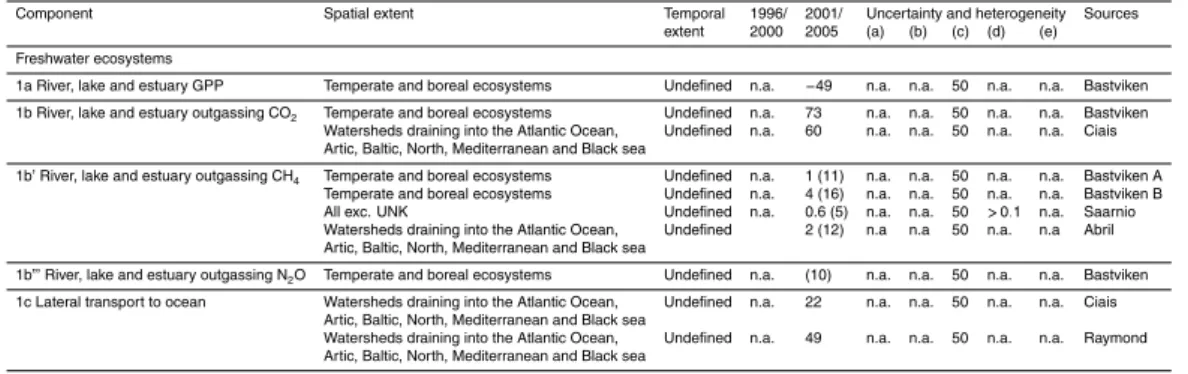
The area under study (Fig. 1) was limited to Europe defined as the landmass containing the EU-27 plus Albania, Bosnia and Herzegovina, Croatia, Iceland, Kosovo, Macedo-nia, Norway, Serbia and Montenegro and Switzerland. A geographical rather than a 5
political definition was followed, therefore, overseas territories (e.g. French Guyana) and distant islands (e.g. Spitsbergen, Canary Islands) where excluded from the carbon and GHG budgets whenever possible. It is often not clear whether the fluxes and stock changes from these islands are included in the data products underlying the carbon and GHG budgets. However, this resulted in minor inconsistencies in the spatial extent 10
of the region under study. Also, it is often unclear whether the data for Serbia and Montenegro include Kosovo or not. We assumed they did not and whenever needed applied a bias correction for Kosovo. For each data product, the known anomalies in the spatial extent are indicated in Table 1.
Geographical Europe typically extends as far as the Ural Mountains and thus in-15
cludes Belarus, Ukraine, the Caucasian republics and part of Russia. Under the RE-CAPP initiative these states are subject of a separate synthesis included in this series (Dolman et al., 2012).
Where data availability permitted, carbon and GHG budgets were estimated for two arbitrary time periods i.e. 1996–2000 and 2001–2005. However, especially for the 20
BGD
9, 2005–2053, 2012The European CO2, CO, CH4 and N2O
balance between 2001 and 2005
S. Luyssaert et al.
Title Page
Abstract Introduction
Conclusions References
Tables Figures
◭ ◮
◭ ◮
Back Close
Full Screen / Esc
Printer-friendly Version
Interactive Discussion
Discussion
P
a
per
|
Dis
cussion
P
a
per
|
Discussion
P
a
per
|
Discussio
n
P
a
per
|
2.2 Accounting framework for GHG budgets
An accounting framework was developed to infer the C-flux between terrestrial ecosys-tems and the atmosphere (Fig. 2). The framework is based on a mass balance ap-proach and given that for Europe most of the components have been independently estimated, different accounting schemes may be used to estimate the variable of inter-5
est i.e. the net land-atmosphere exchange. In this study we applied three, largely in-dependent, accounting schemes based on: (1) atmospheric inversions, (2) land-based flux measurements and (3) land-based carbon inventories.
In the inversion approach the net land-atmosphere exchange is calculated through optimizing a prior land-atmosphere flux where the prior is adjusted to match the ob-10
served atmospheric CO2, CO, CH4 or N2O concentrations. Following the notation
introduced in Fig. 2 and Table 1 this can be formalized for CO2as:
Net land−atmosphere flux = 14a (1)
Where, flux 14a (Fig. 2) represents the change in atmospheric CO2 as derived from
the inversions. In the land-based approaches the change in C stock can be estimated 15
from flux-based estimates the different components of the budget or alternatively, some of the fluxes can be estimated from repeated C-inventories. These approaches are respectively formalized as:
Net land−atmosphere flux = 7e + 1a + 1b +2a + 2b + 2d + 2e + 2f + 2g
+ 2h + 3e + 7a + 4a + 4b + 5a +6b + 6c +6a (2) 20
BGD
9, 2005–2053, 2012The European CO2, CO, CH4 and N2O
balance between 2001 and 2005
S. Luyssaert et al.
Title Page
Abstract Introduction
Conclusions References
Tables Figures
◭ ◮
◭ ◮
Back Close
Full Screen / Esc
Printer-friendly Version
Interactive Discussion
Discussion
P
a
per
|
Dis
cussion
P
a
per
|
Discussion
P
a
per
|
Discussio
n
P
a
per
|
C-gasses (14a′ and 14a′′) have been estimated allowing us to calculate the following component fluxes of Eq. (2):
1a + 1b = 1c + 1b′ −2c −6a −6d −7f −9j (3)
2a + 2b +2d + 2e + 2f +2g + 2h = 2c + 2d′ + 2d′′′ +2i +2kl + 2m
+3a + 3b +7c + 7d −7g − 9a − 9b − 9c − 9d − 9e − 9f −9g − 9i (4) 5
3e=−10a−10b−11−3b+3c−3d+3e′ (5)
7a=−1b′−2d′−2d′′′−2i−2kl−2m−3e′
−4a′−4a′′−4b′−4b′′−5a′−5a′′−6b′+7b−7c−14a′−14a′′ (6)
Substitution of Eqs. (3) to (6) in Eq. (1) results into the following expression for the inventory-based net land-atmosphere flux:
10
Net land−atmosphere flux = 7e+(1c+1b′−2c−6a−6d−7f−9j)+(2c+2d′+2d′′′
(+2i+2kl+2m+3a+3b+7c+7d−7g−9a−9b−9c−9d−9e−9f−9g−9i)+
(−10a−10b−11−3b+3c−3d+3e′)+(−1b′−2d′−2d′′′−2i−2kl−2m−3e′
−4a′−4a′′−4b′−4b′′−5a′−5a′′−6b′+7b−7c−14a′−14a′′)
+4a+4b+5a+6b+6c+6a (7a) 15
or following elimination of terms
Net land−atmosphere flux = 1c+3a+3c−3d+4a−4a′−4a′′+4b−4b′−4b′′
+5a -5a’ -5a”+6b -6b’+6c -6d+7b+7d+7e -7f -7g -9a -9b -9c -9d -9e -9f -9g
BGD
9, 2005–2053, 2012The European CO2, CO, CH4 and N2O
balance between 2001 and 2005
S. Luyssaert et al.
Title Page
Abstract Introduction
Conclusions References
Tables Figures
◭ ◮
◭ ◮
Back Close
Full Screen / Esc
Printer-friendly Version
Interactive Discussion
Discussion
P
a
per
|
Dis
cussion
P
a
per
|
Discussion
P
a
per
|
Discussio
n
P
a
per
|
Given that several inversions used land surface models to derive the prior fluxes and their errors are and that these models are often calibrated and validated against diff er-ent subsets of eddy-covariance data (see for example Bousquet et al., 2010), many inversion-based and flux-based accounting schemes are not entirely independent. However, the assumptions and subsequent post-processing of the eddy-covariance 5
observations differed substantially resulting in quasi-independent schemes. Also CO2
inversion and inventory-based schemes share their data sources for fossil fuel emis-sions and are therefore not entirely independent for this study.
The same mass balance approach can be applied to estimate the C and GHG sink in ecosystems and biological product pools. Also these sinks could be estimates follow-10
ing three quasi-independent approaches: inversion-based, flux-based and inventory-based. Following the notation introduced in Fig. 2 and Table 1 this can be formalized for C as:
Inversion−based C−sink = 14a+14a′+14a′′−7e−4a−4a′−4a′′ (8) −4b−4b′−4b′′−5a−5a′−5a′′+6a−6b−6c
15
Flux−based C−sink = (−2c−7f+1a+1b+1b′+1c+6a−6d)(2ab+2c+2d+2d′+
+2d′′+2e+2f+2g+2h+2i+2k+2l+3a+3b+7c+7d−7g)+(−3b+3d+3c+3e+3e′+2m) (9)
Inventory - based C - sink =9a+9b+9c+9d+9e+9f+9g+9i+9j+10a+10b+11 (10)
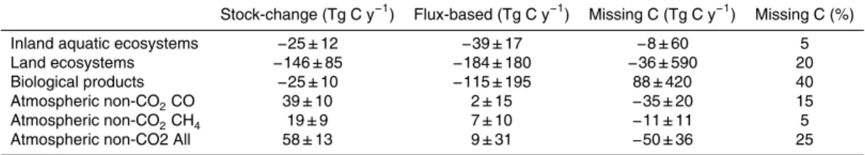
2.3 Balance closure
20
The mass balance approach introduced in Sect. 2.2 supports internal consistency checks. Stock-based changes in carbon content of inland aquatic ecosystems, land ecosystems, biological products and atmospheric pools obtained from inventories or inversions were confronted with their flux-based equivalents. This approach is formal-ized for in Eq. (3) for inland aquatic ecosystems, Eq. (4) for land ecosystems, Eq. (5) 25
BGD
9, 2005–2053, 2012The European CO2, CO, CH4 and N2O
balance between 2001 and 2005
S. Luyssaert et al.
Title Page
Abstract Introduction
Conclusions References
Tables Figures
◭ ◮
◭ ◮
Back Close
Full Screen / Esc
Printer-friendly Version
Interactive Discussion
Discussion
P
a
per
|
Dis
cussion
P
a
per
|
Discussion
P
a
per
|
Discussio
n
P
a
per
|
2.4 Boundaries of the GHG budget
The GHG budget is determined by three boundaries: the spatial, the temporal and the accounting boundary. In this study we used a single spatial boundary (see Sect. 2.1) and two temporal boundaries (see Sect. 2.1). The accounting boundary describes the components that are included in the budget (Fig. 2). However, each of the in-5
cluded components has its own spatial boundaries (e.g. depth to which soil carbon is measured in inventory studies) and its own accounting boundaries. Given that these boundaries are often method-dependent, we choose to specify them in the supplemen-tary material describing the data products (see supplemensupplemen-tary material).
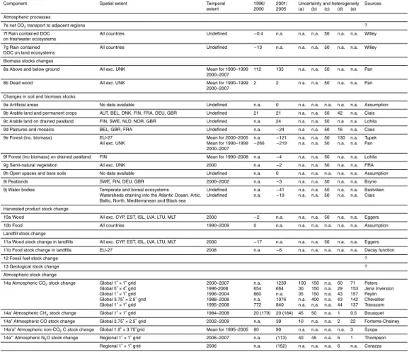
2.5 Data products
10
All data products used in this study are described in the supplementary material provid-ing details on the underlyprovid-ing observations, processprovid-ing done by the data owner, uncer-tainty estimates and post-processing in this study in addition to literature references.
2.6 Uncertainty estimates and error propagation
For data products that were subject of a formal uncertainty analysis, these uncertainty 15
estimates were propagated in the balance computations. However, for the vast majority of the data products, no formal uncertainty analysis was available, for those products we assumed a normal uncertainty distribution with 95 % uncertainty interval amounting to 100 % of the flux estimate (thus 1 standard deviation is 50 % of the flux estimate). This imposed uncertainty was also propagated in the balance computations.
20
BGD
9, 2005–2053, 2012The European CO2, CO, CH4 and N2O
balance between 2001 and 2005
S. Luyssaert et al.
Title Page
Abstract Introduction
Conclusions References
Tables Figures
◭ ◮
◭ ◮
Back Close
Full Screen / Esc
Printer-friendly Version
Interactive Discussion
Discussion
P
a
per
|
Dis
cussion
P
a
per
|
Discussion
P
a
per
|
Discussio
n
P
a
per
|
aggregated flux of the region under study. The heterogeneity estimates are simply reported but not used in any of the uncertainty estimates.
For flux components with a single uncertainty component, the probability distribution was assumed to be normal with mean and standard deviation equal to the reported values. The probability distribution of the uncertainty of the CO2, CO, CH4 and N2O 5
inversions is often reported by two components. The first component describes a quasi uniform range of likely model outputs and is derived from sensitivity analyses (Table 1). The second component describes a normally distributed uncertainty and is due to the set-up of the inversion model and is typically obtained through the Bayesian approach. Within an inversion these components depend on each other and the former should be 10
contained in the latter, if the latter is well-defined. We used the uncertainty that resulted in the widest uncertainty intervals.
Probability distributions were fully accounted for in the balance sheets by means of simulations based on Monte Carlo techniques. Within each realization of the 6000 Monte Carlo simulations that were performed, (sub)totals were computed from 15
randomly selected realizations of the component fluxes. Mean and standard deviations of the (sub)totals were taken from their probability distribution based on 6000 realiza-tions.
2.7 Life cycle analysis
We performed a basic country-based life cycle analysis of the CO2 cost of land man-20
agement including the following processes: (a) agricultural activities (ploughing, har-rowing, cultivation and planting), (b) production and application of fertilizer, (c) produc-tion and applicaproduc-tion of herbicide (glyphosate), (d) thinning, harvesting and planting of forest, (e) transport of roundwood and (f) transport of fire wood. Emission factors were retrieved from Ecoinvent database (Frischknecht et al., 2007). Fertilizer and herbicide 25
BGD
9, 2005–2053, 2012The European CO2, CO, CH4 and N2O
balance between 2001 and 2005
S. Luyssaert et al.
Title Page
Abstract Introduction
Conclusions References
Tables Figures
◭ ◮
◭ ◮
Back Close
Full Screen / Esc
Printer-friendly Version
Interactive Discussion
Discussion
P
a
per
|
Dis
cussion
P
a
per
|
Discussion
P
a
per
|
Discussio
n
P
a
per
|
the time frame of the study, this inconsistency was though to be of minor importance given the assumptions made in the life cycle analysis.
For cropland the following assumptions were made: each cropland is ploughed, har-rowed, planted, cultivated, fertilized, sprayed and harvested annually. Grassland is ploughed and harrowed every 10 yr and cultivated and fertilized every year. In the ab-5
sence of specific data, the CO2 cost of fertilizer production was distributed over crop
and grassland assuming that grasslands received half the dose of croplands. One per-cent of the forest land was harvested and planted and 10 % was thinned each year. The harvested wood was transported over a distance of 80 km if used as industrial roundwood. Fire wood was transported over a distance of 40 km.
10
3 Results and discussion
3.1 Inversion-derived net land-atmosphere GHG fluxes
A subset of inversions, optimized for Europe was selected to compile the European CO2, CH4, CO and N2O budgets (Tables 1 and 2). Despite the effort in harmonizing
the spatial, and temporal extent, the different inversions resulted in largely different 15
estimates of the land-atmosphere flux ranging from 654 Tg C y−1 to 1239 Tg C y−1 for CO2(Chevallier et al., 2010; Peters et al., 2010; Peylin et al., 2005; R ¨odenbeck et al.,
2003). For N2O the two available inversions converged within 25 % from each other.
Although at first this looks very encouraging it should be noticed that both inversions largely used the same observations (Corazza et al., 2011; Thompson et al., 2011) so 20
that the difference between the inversions is most likely due to differences in atmo-spheric transport and the definitions for prior uncertainties. For CH4 (Bousquet et al., 2006) and CO (Fortems-Cheiney et al., 2011) just a single inversion was used and therefore inter-model variability could not be estimated. Further, inversions provide only a top-down estimate for regions constrained by the observations. For N2O the 25
BGD
9, 2005–2053, 2012The European CO2, CO, CH4 and N2O
balance between 2001 and 2005
S. Luyssaert et al.
Title Page
Abstract Introduction
Conclusions References
Tables Figures
◭ ◮
◭ ◮
Back Close
Full Screen / Esc
Printer-friendly Version
Interactive Discussion
Discussion
P
a
per
|
Dis
cussion
P
a
per
|
Discussion
P
a
per
|
Discussio
n
P
a
per
|
The land-atmosphere flux of GHG’s determines to a large extent the rate of ac-cumulation of GHG’s in the atmosphere and its interannual variability modulates the year-to-year growth-rate of GHG’s and is thus of special interest to the climate system. Also interannual variability hints at the sensitivity of the land surface to climate variabil-ity and therefore in hindsight about future land surface responses to climate change. 5
The interannual variability of Europe was studied by simultaneously considering two characteristics: (1) the absolute value of the land-atmosphere fluxµj(µi(| Fluxi j|)) and (2) the mean interannual variability of the land-atmosphere fluxµj(σi(|Fluxi j|)). Where
i indicates the pixel andj indicates the data product. The first characteristic identifies regions where the land-atmosphere flux is potentially important for the climate system 10
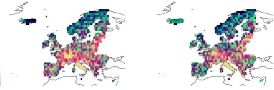
whereas the second characteristic identifies regions where the interannual variability is expected to be large. Combining both characteristics in a single variable (Fig. 3) allows the regions to be distinguished that contribute most to the year-to-year variability in atmospheric CO2concentration.
For both periods (1996–2000 and 2001–2005), the net land-atmosphere flux in Scan-15
dinavia is a small contributor and the central region appears as an important contributor to the interannual variability in atmospheric CO2 concentration over Europe. A simi-lar latitudinal pattern in interannual variability was observed for deciduous forests but contradicted for evergreen forest based on observations from 39 northern-hemisphere eddy-covariance sites located at latitudes ranging from 29oN to 64◦N (Yuan et al., 20
2009). A comparison between two deciduous and one evergreen site suggests that deciduous forests may contribute disproportionately to variability in atmospheric CO2
concentrations within the northern hemisphere (Welp et al., 2007). Given the higher abundance of deciduous forests in central and southern compared to northern Europe, this finding may help to explain the observed spatial pattern (Fig. 3) in interannual vari-25
BGD
9, 2005–2053, 2012The European CO2, CO, CH4 and N2O
balance between 2001 and 2005
S. Luyssaert et al.
Title Page
Abstract Introduction
Conclusions References
Tables Figures
◭ ◮
◭ ◮
Back Close
Full Screen / Esc
Printer-friendly Version
Interactive Discussion
Discussion
P
a
per
|
Dis
cussion
P
a
per
|
Discussion
P
a
per
|
Discussio
n
P
a
per
|
Rather than being an ecosystem property, the interannual variability in ecosystem productivity may be due to differences in weather patterns between central and north-ern Europe. Such a difference could for example be determined by the North Atlantic Oscillation (NAO) (Hoerling et al., 2001). In some years, the NAO pushes the Mediter-ranean climate southward resulting in wet weather in the central and MediterMediter-ranean 5
Europe, other years the NAO allows a more northern occurrence of the Mediterranean climate resulting in dry weather in central Europe (Hurrell, 1995). Differences in the spatial extent of the summer and winter NAO (Linderholm et al., 2009) may contribute to the observed north-south trend in interannual variability of the land-atmosphere CO2
flux. 10
The inversion-derived interannual variability over Europe is sensitive to the lack of observational constraint on fluxes and imperfect knowledge of the prior flux estimates. Atmospheric inversions are forced to achieve mass balance closure. The inversions may achieve mass balance closure by simply attributing the residual fluxes to the least constrained regions. In Europe, the tall tower network that is used to constraint the 15
inversions is less dense in northern, southern and eastern compared to central Europe (Ramonet et al., 2010). Contrary to our observations, this set-up of the inversions is expected assigning the residual fluxes and thus the highest variability to northern and southern Europe. However, in line with the set-up of the inversions, the inversions assigned a high variability to eastern Europe (EST, LVA, LTU and POL), a region poorly 20
constrained by measurements. Therefore, the observed pattern in Eastern Europe could reflect the state of the art in inversion rather than a biological phenomenon.
3.2 Eddy-covariance and inventory-based net land-atmosphere GHG fluxes
3.2.1 Land-use and surface area
The study region has surface area of 5×10⁶km2of which all except Switzerland is be-25
BGD
9, 2005–2053, 2012The European CO2, CO, CH4 and N2O
balance between 2001 and 2005
S. Luyssaert et al.
Title Page
Abstract Introduction
Conclusions References
Tables Figures
◭ ◮
◭ ◮
Back Close
Full Screen / Esc
Printer-friendly Version
Interactive Discussion
Discussion
P
a
per
|
Dis
cussion
P
a
per
|
Discussion
P
a
per
|
Discussio
n
P
a
per
|
most 12 % for the EU-25 when FAO and CORINE are compared. This difference is likely explained by CORINE classifying part of the harvested forest as semi-natural veg-etation. While different sources (i.e. CORINE versus FAO) agree on the importance of forest and cropland (estimates differ at most 6 % for the EU-25), such convergence is absent for grazing land with estimates diverging by more than 20 % for the EU-25, 5
which contains the best documented nations of Europe. This uncertainty is caused by whether the classification of grazing land includes only permanent grasslands (e.g. per-manent pastures) which are intensively and continuously managed (i.e. mowing or grazing) or also natural or semi-natural vegetation that is extensively grazed.
Where the CORINE land cover classes account for wetlands it is important to dis-10
tinguish between marshes and peatland and more specifically between disturbed and undisturbed peatland. For GHG budgets, distinguishing between these management types is essential because the undisturbed peatland typically acts as a GHG-sink whereas the disturbed peatland under cropland and forests often act as a GHG-source because of enhanced decomposition following harvest, ploughing and or drainage. 15
The areas for different land uses on peatland have been taken from Joosten (2010). Although not explicitly reported by Joosten (2010), for this study, the areas were as-sumed constant between 1996 and 2005.
3.2.2 Eddy covariance based net land-atmosphere flux
The current eddy-covariance tower network is equipped to record the CO2 exchange 20
between land and atmosphere (this fluxes is also known as NEE in the sense of Chapin et al., 2005). Although an eddy-covariance based CH4network is emerging, at present
only very few sites report other greenhouse gas fluxes than CO2, therefore, our
eddy-covariance based estimates are limited to CO2exchange.
At the site scale, the scale for which eddy-covariance measurements are avail-25
able, CO2 is exchanged with neighbouring sites (i.e. lateral CO2 transport, harvest
BGD
9, 2005–2053, 2012The European CO2, CO, CH4 and N2O
balance between 2001 and 2005
S. Luyssaert et al.
Title Page
Abstract Introduction
Conclusions References
Tables Figures
◭ ◮
◭ ◮
Back Close
Full Screen / Esc
Printer-friendly Version
Interactive Discussion
Discussion
P
a
per
|
Dis
cussion
P
a
per
|
Discussion
P
a
per
|
Discussio
n
P
a
per
|
ecosystem and atmosphere. Consequently, NEE estimates need to be corrected for lateral transport and leaching from the soil matrix to obtain the ecosystem carbon sink. Accounting is further complicated by the fact that (Korner, 2003): (1) C, CH4and CO2
are exported to neighbouring ecosystems that are not part of the eddy-covariance net-work i.e. inland water and product pools (Fig. 2). Therefore, lateral fluxes and the CO2 5
exchange between these ecosystems and the atmosphere also need to be accounted for. (2) For forests and grasslands the network is biased towards uniform established ecosystems, hence, newly established ecosystems following land-use change need to be separately accounted for. (3) Eddy-covariance measurements are not made during fires to prevent the equipment from being damaged; fires emissions thus need to be 10
separately accounted for. (4) No eddy-covariance network exists over urban and in-dustrial areas, therefore, fossil fuel emissions need to be separately accounted for. (5) The eddy-covariance is not globally representative but given its density over Europe, this is likely a minor issue for estimating mean fluxes over the study region (Sulkava et al., 2011). Equation (2) and Fig. 2 show how issues 1 to 4 were accounted for in this 15
study.
Despite being well documented that annual NEE poorly correlates to climate and is more likely driven by site disturbance such as harvest, grazing, thinning, fire, ploughing, etc. (Luyssaert et al., 2007), for a given site, NEE fluxes at high temporal resolutions (i.e. hourly to monthly) are (partly) driven by meteorology (Baldocchi, 2008; Law et al., 20
2002). Jung et al. (2011) and Papale et al. (2003) used this observation to upscale eddy-covariance measurement to the region. Nevertheless, these authors caution for the lack of spatially explicit disturbance data in their upscaling approach and the sub-stantial uncertainty of their data products (Jung et al., 2009, 2011).
For the region and period under consideration both eddy-covariance-based esti-25
mates (Table 1), using the same data but different statistical methods, converged at −965 Tg C y−1within 10 % (one standard deviation). Not surprisingly the estimates in-dicate that the European land surface consistently takes up CO2from the atmosphere.
BGD
9, 2005–2053, 2012The European CO2, CO, CH4 and N2O
balance between 2001 and 2005
S. Luyssaert et al.
Title Page
Abstract Introduction
Conclusions References
Tables Figures
◭ ◮
◭ ◮
Back Close
Full Screen / Esc
Printer-friendly Version
Interactive Discussion
Discussion
P
a
per
|
Dis
cussion
P
a
per
|
Discussion
P
a
per
|
Discussio
n
P
a
per
|
related to meteorology. Although the spatial variability in NEE is thought to be driven by disturbances, the relationship between the temporal variability in NEE and meteo-rology may be real (Baldocchi, 2008; Law et al., 2002). Nevertheless, the strength of this relationship is most likely an artefact of the fact that the upscaling makes use of remotely sensed fpar and meteorological data (Jung et al., 2011). Following account-5
ing for fluxes not measured by the eddy-covariance technique (Eq. 2), the net land-atmosphere flux was estimated at 943±540 Tg C y−1between 2001 and 2005. Several of the flux estimates were temporally unresolved, hence, the interannual variability of the net land-atmosphere flux could not be estimated.
3.2.3 Inventory based net land-atmosphere flux
10
Alternatively, net land-atmosphere fluxes of CO2, CH4and CO can be estimated from
repeated C-inventories often in conjunction with deterministic models (i.e. Tupek et al., 2010; see also supplementary material) and flux measurements to complete the inventory measurements (see Methods and material). This approach has been formal-ized in Eq. (7). Although this appears as the most straightforward of the three applied 15
approaches to estimate the net land-atmosphere flux, the representativeness of the European estimates may be hampered by data scarcity (see supplementary material). For example, changes in soil carbon for the entire territory are based on a rather limited number of sampling plots for croplands (Ciais et al., 2010c) and grasslands (Lettens et al., 2005; Goidts and Wesemael, 2007; Soussana et al., 2004; Bellamy et al., 2005) 20
and are based on deterministic modelling for forests (Luyssaert et al., 2010; Tupek et al., 2010). Further, spatially explicit estimates are none existent for several potential hotspots such as drained peatlands, reservoirs and areas under land-use change, for example, it remains unclear what happens with soil carbon following urbanisation.
Assuming that the regions that were inventoried are representative for the spa-25
BGD
9, 2005–2053, 2012The European CO2, CO, CH4 and N2O
balance between 2001 and 2005
S. Luyssaert et al.
Title Page
Abstract Introduction
Conclusions References
Tables Figures
◭ ◮
◭ ◮
Back Close
Full Screen / Esc
Printer-friendly Version
Interactive Discussion
Discussion
P
a
per
|
Dis
cussion
P
a
per
|
Discussion
P
a
per
|
Discussio
n
P
a
per
|
is a source for CH4 and CO of respectively 23±5 and 21±5 Tg C y− 1
. For N2O the
land-atmosphere flux is estimated at 125±35 Tg C in CO2-eq y− 1
or 1 Tg N y−1. Sev-eral of the flux estimates required to estimate the net land-atmosphere flux of CO2, CH4, CO and N2O were temporally unresolved, hence, the interannual variability was
not estimated. 5
3.3 Uncertainty and consistency of the net land-atmosphere GHG fluxes
Inversion based accounting adjusts a prior set of fluxes for the net ecosystem-atmosphere exchange with a given uncertainty to better match the observed atmo-spheric concentrations of the species under study within their uncertainty. Recent in-versions come with a formal uncertainty analysis (Table 1). However, the vast majority 10
of the data products other than inversions have not been subjected to formal uncer-tainty analysis. For these products we assumed a Gaussian unceruncer-tainty distribution with 95 % uncertainty interval amounting to 100 % of the flux estimate (thus 1 standard deviation is 50 % of the flux estimate).
The uncertainty of the eddy-covariance and inventory based estimate of the net 15
land-atmosphere flux was estimated from the uncertainty of its components and is thus determined by the assumed uncertainty of 50 %. Despite the shared assump-tion, the uncertainty of the inventory-based estimate was estimated to be almost one third of that of the flux-based estimate (Table 2). This difference is due to the diff er-ence in the magnitude of the fluxes that are used in the balance calculations (i.e. Eq. 2 20
vs. Eq. 7). Given our assumption, the largest component flux comes with the largest uncertainty. Consequently, the total uncertainty is determined by the uncertainty of the upscaled NEE (2ab; Table 1) in the flux-based approach whereas the uncertainty of the inventory-based approach is determined by the uncertainties of fossil fuel burning (5a; Table 1) and the changes in forest carbon (9e; Table 1) . Improved uncertainty 25
BGD
9, 2005–2053, 2012The European CO2, CO, CH4 and N2O
balance between 2001 and 2005
S. Luyssaert et al.
Title Page
Abstract Introduction
Conclusions References
Tables Figures
◭ ◮
◭ ◮
Back Close
Full Screen / Esc
Printer-friendly Version
Interactive Discussion
Discussion
P
a
per
|
Dis
cussion
P
a
per
|
Discussion
P
a
per
|
Discussio
n
P
a
per
|
The mass balance approach introduced in Sect. 2 supports internal consistency checks. Stock-based changes in carbon content of the aquatic, terrestrial, product and atmospheric pool obtained from inventories or inversions were confronted with their flux-based equivalents (Fig. 2). This approach is formalized for CO2 in Eqs. (3) to (6) and the balance closure has been reported in Table 3. Balance closure between 5
the stock-based and flux-based estimates is not significantly different from zero mainly because of the wide uncertainty intervals. The current estimates and their uncertain-ties lack statistical evidence to justify introducing a ‘closure gap’. Hence, our estimates for these components were considered consistent. Consistency is expected to further improve if atmospheric transport to adjacent regions would be accounted for (7b, 7d 10
and 7e in Table 1).
However, when the land sink is used as reference, the statistics-based consistency seems not justified for the biological product pool (i.e. all harvested biomass and subse-quent products such as food, fodder, wood, paper, . . . ) which shows an inconsistency of 88 Tg C y−1between the stock-change and flux-based approach. This inconsistency 15
represents about 40 % of the inventory-based change in carbon stock for the region under study (Table 3). This inconsistency may be due to the lack of dense harvest and herbivory observations for grasslands and croplands. The current budget relies on modelled data (see 3b, c and 3b, d in Table 1). Hence, it is expected that the internal consistency of the European C budget could largely improve by informing emissions 20
estimates of biological product pools by measurements.
It should be noted that in this consistency check, two inaccurate fluxes could com-pensate each other resulting in an apparently high consistency. Consequently, the information content of our balance closure approach is limited as it does not identify which fluxes or stock-change estimates need to be further improved to improve the 25
BGD
9, 2005–2053, 2012The European CO2, CO, CH4 and N2O
balance between 2001 and 2005
S. Luyssaert et al.
Title Page
Abstract Introduction
Conclusions References
Tables Figures
◭ ◮
◭ ◮
Back Close
Full Screen / Esc
Printer-friendly Version
Interactive Discussion
Discussion
P
a
per
|
Dis
cussion
P
a
per
|
Discussion
P
a
per
|
Discussio
n
P
a
per
|
3.4 GHG mitigation of European ecosystems
Sink estimates, based on Eqs. (8) to (10), show that the European ecosystems and bi-ological product pools were a C-sink between−356 and −201 Tg C y−1between 2001 and 2005 (Table 4). Individual sink estimates come with large uncertainties ranging between 80 and 330 Tg C y−1. However, the extreme high and low sink-strengths are 5
in conflict with the inventory-based approach that has a much smaller uncertainty of 80 Tg C y−1 and as such puts a tighter constraint on the estimated sink strength. Ap-plying the Bayesian theorem, a sink of−210±70 Tg C y−1 was found to be consistent with our three independent data sources i.e. atmospheric measurements, observed stock-changes and measured fluxes.
10
This C-sink in European ecosystems and biological product pools is thought to be mainly driven by changes in atmospheric CO2, climate, atmospheric N-deposition, land
use (intensity) change and to a minor extent by changes in ozone concentration and diffuse versus direct light flux (Le Qu ´er ´e et al., 2009). Proper understanding of the drivers, their interaction and their contributions to the current sink is a prerequisite to 15
predict whether the current sink-strength will increase, decrease or persist in the future. Spatially explicit sink attribution at the European scale is beyond the capacity of exper-imental work and can only be achieved by well-validated model-based experiments. For example, model-based experiments could shed a light on the effect of large scale bio-energy production on the current sink-strength. Such modelling-experiments could 20
extent the time period of data-driven studies (for example Hudiburg et al., 2011). How-ever, model-based sink attribution is still in its infancy because currently no single large scale model can deal with all aforementioned factors. At present multiple model-based experiments have been performed with different models. Hence, the observed sink is attributed to just a limited number of drivers, likely overestimating the importance of the 25
drivers the model accounts for.
BGD
9, 2005–2053, 2012The European CO2, CO, CH4 and N2O
balance between 2001 and 2005
S. Luyssaert et al.
Title Page
Abstract Introduction
Conclusions References
Tables Figures
◭ ◮
◭ ◮
Back Close
Full Screen / Esc
Printer-friendly Version
Interactive Discussion
Discussion
P
a
per
|
Dis
cussion
P
a
per
|
Discussion
P
a
per
|
Discussio
n
P
a
per
|
European C-sink than climate (Harrison et al., 2008b). Note that Europe was here de-fined as continental Europe. Warming was reported to emit C to the atmosphere. This C-source, however, was more than offset by the effect of increasing atmospheric [CO2]
resulting in a −114 Tg C y−1 sink between 1980–2005 (Harrison et al., 2008a). This modelling-experiment likely overestimates the effects of climate change and increasing 5
[CO2] because it accounted for land-use (intensity) change, N-deposition, increasing
atmospheric ozone and diffuse vs. direct light.
Another model experiment performed with a version of the LPJ (Lund Potsdam Jena) land surface model) accounting for climate change, increasing atmospheric [CO2]
and land cover change, found an important effect of land use change over the EU-10
15 (Zaehle et al., 2007). During the 1990’s, 3.3 Tg C y−1 was lost to urbanization, 19.3 Tg C y−1 to agricultural and 14.5 Tg C y−1 to grasslands. Emission due to land cover change were offset by sequestration of−59.1 Tg C y−1 in forest and wood prod-ucts resulting in a mean annual C-sink of−29 Tg C y−1(Zaehle et al., 2007).
O-CN, a branch of ORCHIDEE (Organizing Carbon and Hydrology in Dynamic 15
Ecosystems) integrating climate change, increasing atmospheric [CO2] and the
ni-trogen cycle, shows that nini-trogen deposition considerably alters the attribution of the C-sink to its drivers. Including nitrogen dynamics limited the global sink-strength by al-most 0.4 Pg C y−1 in the N-limited boreal regions, whereas N-deposition was reported to enhance the global terrestrial C-sink by 10 to 20 % (i.e.−0.2 to−0.4 Pg C y−1). Given 20
that no N-effect was simulated for tropical regions, interactions with reactive nitrogen (Nr) substantially contribute to the C-sink in the temperate zone (Zaehle et al., 2010). A similar modelling-experiment using a slightly different version of O-CN that also ac-counts for the effects of land cover change .(Zaehle et al., 2011) resulted in a net forest uptake rate due to Nr deposition of 23.5±8.5 Tg C y−1(mean and standard deviation of 25
BGD
9, 2005–2053, 2012The European CO2, CO, CH4 and N2O
balance between 2001 and 2005
S. Luyssaert et al.
Title Page
Abstract Introduction
Conclusions References
Tables Figures
◭ ◮
◭ ◮
Back Close
Full Screen / Esc
Printer-friendly Version
Interactive Discussion
Discussion
P
a
per
|
Dis
cussion
P
a
per
|
Discussion
P
a
per
|
Discussio
n
P
a
per
|
thereafter remained relatively constant with some inter-annual variations related mainly to the interactions of Nr availability with climatic variability (Zaehle et al., 2011).
A comparison of BIOME-BGC (Global Biome model – Biogeochemical Cycles), JULES, ORCHIDEE and O-CN suggested a continuous increase in carbon storage from 85 Tg C y−1in 1980s to 108 Tg C y−1in 1990s, and to 114 Tg C y−1in 2000–2007 5
(Churkina et al., 2010). These estimates are for continental Europe and limited to the terrestrial ecosystems sink. The study identified the effect of rising [CO2] in
combina-tion with Nr-deposicombina-tion and forest re-growth as the important explanatory factors for this net carbon storage. However, the modelling-experiments did not account for changes in the age structure of woody vegetation, a potentially important contributor.
10
Some modelling-experiments zoomed in on a single ecosystem and its specific char-acteristics. The effect of changes in age structure of forest has been subjected to sep-arate modelling-experiments (Bellassen et al., 2011; Zaehle et al., 2006). For Europe, ORCHIDEE-FM, another branch of ORCHIDEE, integrating climate change, increas-ing atmospheric [CO2], net forest cover change and changing age structure of forest 15
shows spatial variation in the main drivers. Locally, climate change and changing age structure often determine temporal changes in the forest C-sink, whereas at the conti-nental scale, increasing atmospheric [CO2] drives the increase of the forest sink
(Bel-lassen et al., 2011). A modelling-experiment with a similar capacity but making use of a LPJ (Zaehle et al., 2006) instead of ORCHIDEE-FM (Bellassen et al., 2011) found 20
that climate change and increased atmospheric [CO2] resulted in a net increase in the
vegetation carbon stock of −57 Tg C y−1 in the 1990s over the EU-25. Afforestation doubled the sink strength by−118 Tg C y−1. Despite its local importance for determin-ing the carbon balance on the European scale, changes in harvest intensity decreased C-sequestration by 5 Tg C y−1in forest vegetation and thus had a small impact on the 25
BGD
9, 2005–2053, 2012The European CO2, CO, CH4 and N2O
balance between 2001 and 2005
S. Luyssaert et al.
Title Page
Abstract Introduction
Conclusions References
Tables Figures
◭ ◮
◭ ◮
Back Close
Full Screen / Esc
Printer-friendly Version
Interactive Discussion
Discussion
P
a
per
|
Dis
cussion
P
a
per
|
Discussion
P
a
per
|
Discussio
n
P
a
per
|
Contrary to the inventory-based estimates (Table 1), model simulations estimated a small but uncertain CO2 C-sink in croplands (Ciais et al., 2010b). This sink was
attributed mainly to past and current management, and to a minor extent the shrinking areas of arable land consecutive to abandonment during the 20th century (Ciais et al., 2010b). When assessing the effects of rising atmospheric [CO2], changing climate, 5
and technology changes on the carbon balance of European croplands, agro-technology changes and varieties selection were found to be largely responsible for the sink rather than rising [CO2] and climate change (Gervois et al., 2008). Sink uncertainty
for croplands was dominated by unknown historical agro-technology changes (Ciais et al., 2010b; Kutsch et al., 2010; Ceschia et al., 2010) and model structure (Ciais et al., 10
2010b) with the model potentially missing processes that contribute to the observed C-source i.e. ploughing. Errors in climate forcing played a minor role (Ciais et al., 2010b). The above mentioned modelling-experiments limited their simulations to CO2uptake
and emissions. However, the same European ecosystems and biological product pools that were a CO2-sink were a source for CH4, CO and N2O (Table 2). When converted 15
to a common unit i.e. Tg C in CO2-eq y− 1
the C-sink is most likely offset by the global warming potential of CH4and N2O. As a consequence, the European ecosystems and biological product pools are a GHG source of 105 ±100 Tg C in CO2-eq y−1 to the atmosphere and thus contribute to global warming (Table 4). This finding confirms previous data-driven (Schulze et al., 2009, 2010) and model-based (Zaehle et al., 20
2011) studies.
To our best knowledge there are no comprehensive attribution studies of the GHG balance, which for Europe appears to be a source of GHG to the atmosphere (Ta-ble 4). However, global GHG-species-specific studies possibly shed some light on the global drivers of N2O and CH4emissions. Before 1960, agricultural expansion, includ-25
BGD
9, 2005–2053, 2012The European CO2, CO, CH4 and N2O
balance between 2001 and 2005
S. Luyssaert et al.
Title Page
Abstract Introduction
Conclusions References
Tables Figures
◭ ◮
◭ ◮
Back Close
Full Screen / Esc
Printer-friendly Version
Interactive Discussion
Discussion
P
a
per
|
Dis
cussion
P
a
per
|
Discussion
P
a
per
|
Discussio
n
P
a
per
|
for Europe.
The emissions of atmospheric methane were investigated by using two atmospheric inversions to quantify the distribution of sources and sinks for the 2006–2008 pe-riod, and a process-based model of methane emissions by natural wetland ecosys-tems (Bousquet et al., 2010). At the global scale, a significant contribution of CH4 5
emissions was thought to come from wetlands in Eurasia where annual changes in precipitation where thought to be the underlying driver (Bousquet et al., 2010). How-ever, other studies put forward other drivers i.e. more efficient rice production (Fuu Ming et al., 2011), unlikely to be important for Europe, or changes in petroleum production and use (Aydin et al., 2011). It remains to be quantified how relevant these global 10
drivers are in explaining the European CH4emissions.
Integrated studies of the interactions of carbon (i.e. CO2, CH4, BVOC, CO) and
nitro-gen (N2O) dynamics, land use (intensity) changes and environmental changes (i.e.
in-creasing atmospheric [CO2], climate change, increasing [O3], changes in direct versus diffuse light) are needed to further improve the quantitative understanding of the driving 15
forces of the European land carbon balance. Although such simulations may become available within a couple of years for forest, grasslands or croplands, a single simulation simultaneously accounting for the different ecosystems (including aquatic ecosystems) may not be available within the next 5 yr or so. The major constraints in realizing such simulations are: (a) model development in of support of such simulations and (b) lack 20
of multi-factorial field experiments that can be used to validate such model outcome.
3.5 Fossil fuel cost of the C sinks
The carbon sink is often presented as a free service from “nature” to “mankind” and in this section we test whether this statement is justified for the Europe. It has been shown that land management is among the main drivers of the European ecosystem-25
BGD
9, 2005–2053, 2012The European CO2, CO, CH4 and N2O
balance between 2001 and 2005
S. Luyssaert et al.
Title Page
Abstract Introduction
Conclusions References
Tables Figures
◭ ◮
◭ ◮
Back Close
Full Screen / Esc
Printer-friendly Version
Interactive Discussion
Discussion
P
a
per
|
Dis
cussion
P
a
per
|
Discussion
P
a
per
|
Discussio
n
P
a
per
|
and product use CO2”, 4a “Peat, wood and charcoal burning CO2” and 4b “other bio-fuel burning CO2”. In this section we used life cycle analysis (LCA) to estimate how
much of the CO2 emitted through fluxes 4a and 4b and 5a can be allocated to land
management.
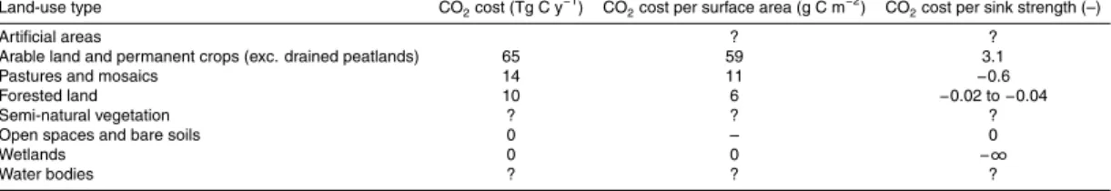
Based on our LCA assumptions (see Sect. 2.6) we estimated that the CO2 cost 5
for ecosystem management is 65 Tg C y−1 for cropland, 14 Tg C y−1for grassland and 10 Tg C y−1for forest (Table 5). Total emission for land management is thus 89 Tg C y−1 which represents less than 10 % of the total European emissions from fossil fuel burn-ing. However, when the land sink rather than the fossil fuel emissions are used as a reference, emissions due to land management practices (i.e. ploughing, harvesting, 10
fertilizing, etc.) can no longer be ignored.
Current agricultural ecosystems are a source of 21 Tg C y−1 (Table 1) and to create this source another 65 Tg C y−1is emitted through energy use for land management (in-cluding fertilizer and herbicide production and application). Management of grasslands is a small sink: the ecosystems store about 24 Tg C y−1their management emits about 15
14 Tg C y−1. Forest management is doing considerably better: only 0.02 and 0.04 Tg of C are emitted to sequester 1 Tg C in the ecosystem. We hypothise that in addition to fossil fuels consumed to manage the forest C-sink, the sink strength in European forests is an indirect result of high fossil fuel consumption, as has been shown for Aus-tria (Erb et al., 2008; Gingrich et al., 2007). Part of the current forest sink is thought 20
to be a result of society’s decreasing dependency on forest biomass resulting in har-vest levels well below wood increment. This situation is maintained by the fact that the energy and raw material previously provided by forests has now been substituted by fossil fuel based energy and products.
It should be noted that undisturbed peatlands are observed to be C-sinks (Table 1) 25
BGD
9, 2005–2053, 2012The European CO2, CO, CH4 and N2O
balance between 2001 and 2005
S. Luyssaert et al.
Title Page
Abstract Introduction
Conclusions References
Tables Figures
◭ ◮
◭ ◮
Back Close
Full Screen / Esc
Printer-friendly Version
Interactive Discussion
Discussion
P
a
per
|
Dis
cussion
P
a
per
|
Discussion
P
a
per
|
Discussio
n
P
a
per
|
Rivers, lakes and reservoirs act as C-sinks (Table 1) but the structure of their manage-ment cost is somehow different from terrestrial ecosystems as it constitutes mainly of the cost for constructing canals and dams of which we had insufficient information to estimate their cost.
It should be noted that our cost analysis was strictly limited to ecosystem manage-5
ment. Hence, subsequent processing of the food and raw material was not included. Such inclusion is likely to change the outcome of the LCA substantially. The CO2cost for food processing in the EU-27 is at least 12 Tg C y−1between 2001 and 2005 (item 1.AA.2.E in UNFCCC, 2007) and thus relatively low compared to its production costs. The CO2cost of wood processing and especially pulp and paper production, is with 8 10
Tg C y−1between 2001 and 2005 (item 1.AA.2.D in UNFCCC, 2007) high compared to the production cost of the wood itself. Also the CO2 costs for managing the biological
product pool are expected to be substantial but not included in this LCA. Given the as-sumptions and the accounting boundary of this LCA, the results should be considered as indicative rather than final. Nevertheless it clearly demonstrates the point that the 15
European C-sink in ecosystems and biological product pools is not a free service but comes at a considerable CO2cost.
4 Conclusions
This study confirmed that the European land surface (including inland waters and ur-ban areas) is a net source for CO2, CO, CH4 and N2O. However, for all ecosystems 20
except croplands, C uptake exceeds C release and us such part of the CO2 released
through fossil fuel burning is removed from the atmosphere and sequestered in both terrestrial and inland aquatic ecosystems. Note that the aquatic systems are estimated to contribute second most to fossil fuel uptake, and thus rank above the European crop-lands and grassland. Given their surface area, this makes the inland waters a hotspot 25
BGD
9, 2005–2053, 2012The European CO2, CO, CH4 and N2O
balance between 2001 and 2005
S. Luyssaert et al.
Title Page
Abstract Introduction
Conclusions References
Tables Figures
◭ ◮
◭ ◮
Back Close
Full Screen / Esc
Printer-friendly Version
Interactive Discussion
Discussion
P
a
per
|
Dis
cussion
P
a
per
|
Discussion
P
a
per
|
Discussio
n
P
a
per
|
If global CO2uptake would be uniformly distributed over the globe, the region under study is expected to sequester−45 to−105 Tg C y−1. Based on three independent ap-proaches we estimated the European C sequestration to amount−210±70 Tg C y−1. Owing to its large uncertainty, the additional uptake of 96 to 156 Tg C was not statis-tically significant but was nevertheless seen as an indicator that the European land 5
surface (including inland waters) takes up more C than the global average. Along the same lines of reasoning, the region under study represents less than 4 % of global photosynthesis but realizes 8 to 18 % of the global C-sink.
If the C cost for ecosystem management is taken into account, the net uptake of ecosystems was estimated to decrease by 45 % but still indicates substantial C-10
sequestration. Also, when the balance is extended from CO2towards the main GHGs, C-uptake by terrestrial and aquatic ecosystems is compensated for by emissions of GHGs. As such the European ecosystems are unlikely to contribute to mitigating the effects of climate change.
Until present it appears impossible to estimate independent temporally resolved 15
GHG balances over Europe for 1991–2000 and 2001–2009 due to lack of data. For several of the fluxes, all available data needed to be combined in a single and therefore temporally undefined estimate. We assigned our estimate to the period 2001–2005 but made use of data from other time periods. Hence, we did not succeed in obtaining high temporal consistency as stated in the objectives of this study and therefore temporal 20
patterns in the GHG balance are not supported by this data compilation.
Achieving high spatial consistency, another objective of this study, was reasonably well achieved as most data products come with a well defined spatial extent, however, it remains unclear whether all products could be considered representative for the whole spatial domain as often only subregion(s) of the under study were sampled. These 25