Ocean parameter estimation with high-frequency signals using a vector sensor array

(1)

Faculdade de Ciˆ

encias e Tecnologia

Ocean Parameter Estimation

with High-frequency Signals using

a Vector Sensor Array

Mestre Paulo Jorge Maia dos Santos

Tese apresentada à Universidade do Algarve para a obten¸cão do grau de Doutor no ramo de Engenharia Electrónica e Telecomunica¸cões, especialidade Processamento de Sinal.

(2)

(3)

Faculdade de Ciˆ

encias e Tecnologia

Ocean Parameter Estimation

with High-frequency Signals using

a Vector Sensor Array

Mestre Paulo Jorge Maia dos Santos

Orientadores: Doutor Sérgio Manuel Machado Jesus, Professor Catedrático da Faculdade de Ciências e Tecnologia, Universidade do Algarve

Doutor Paulo Alexandre da Silva Felisberto, Professor Adjunto do Instituto Superior de Engenharia, Universidade do Algarve

Tese apresentada à Universidade do Algarve para a obten¸cão do grau de Doutor no ramo de Engenharia Electrónica e Telecomunica¸cões, especialidade de Processamento de

Sinal.

(4)

Ocean Parameter Estimation with High-frequency Signals

using a Vector Sensor Array

Declara¸c˜ao de autoria do trabalho

Declaro ser o autor deste trabalho, que é original e inédito. Autores e trabalhos consultados estão devidamente citados no texto e constam da listagem de referências bibliográficas inclu´ıda.

Copyright c Paulo Jorge Maia dos Santos

A Universidade do Algarve tem o direito, perpétuo e sem limites geográficos, de arquivar e publicitar este trabalho através de exemplares impressos repro-duzidos em papel ou de forma digital, ou por qualquer outro meio conhecido ou que venha a ser inventado, de o divulgar através de repositórios cient´ıficos e de admitir a sua cópia e distribui¸cão com objectivos educacionais ou de investiga¸cão, não comerciais, desde que seja dado crédito ao autor e editor.

(5)

(6)

I

`

A minha filhota Rita que deu os primeiros passos no in´ıcio do meu tra-balho de Doutoramento

e cresceu ao mesmo tempo que o tra-balho desta Tese evolu´ıa,

ao meu filho Francisco pela paciˆencia que teve ao longo destes anos,

e `a minha mulher Sandra pelo apoio in-condicional e compreens˜ao nos momen-tos mais dif´ıceis.

(7)

(8)

III

Acknowledgements

I would like to thank my supervisors Prof. S´ergio M. Jesus and Prof. Paulo Felisberto for their permanent effort in providing the necessary conditions in the laboratory for accomplishing the objectives of this work, by organizing scientific projects and sea trials for collecting experimental data, their useful advises, and in particular, for their contributions through many suggestions and comments during the writing of this thesis.

I would like to thank also Prof. Orlando Rodr´ıguez for the design of the TRACEO Gaussian beam model used in this work, which provides the particle velocity outputs, and for his help, advises, comments and suggestions during the writing of this thesis.

I thank my colleagues in Electrotecnic Engineering Depart-ment of the ISE, University of Algarve for giving me conditions to realize the work of this thesis. Thank also my colleagues in the Signal Processing Laboratory (SiPLAB) that daily contributed for an enjoyable social environment and their contributions to the work of this thesis.

I would like to thank Michael Porter, chief scientist for the Makai Experiment, Jerry Tarasek at Naval Surface Weapons Center for the loan of the vector sensor array used in this work. I also thank Bruce Abraham at Applied Physical Sciences for providing assistance with the data acquisition and the team at HLS Research, particularly Paul Hursky for their help with the data used in this work.

Finally, special thanks to my wife and my children, for their patience and support, specially during the writing of this thesis.

This work was partially funded by National Funds through FCT - Fundation for Science and Technology under project SENSOCEAN (PTDC/EEA-ELC/104561/2008).

(9)

(10)

V

Name: Paulo Jorge Maia dos Santos College: Faculdade de Ciˆencias e Tecnologia University: Universidade do Algarve

Supervisors: Doutor S´ergio Manuel Machado Jesus, Full Professor of Faculdade de Ciˆencias e Tecnologia, Universidade do Algarve and Doctor Paulo Alexandre da Silva Felisberto, Adjoint Professor of Instituto Superior de Engenharia, Universidade do Algarve

Thesis title: Ocean Parameter Estimation with High-frequency Signals using a Vector Sensor Array

Abstract

Vector sensors began to emerge in 1980s as potential competitors to omni directional pressure driven hydrophones, while their practical usage in un-derwater applications started in the last two decades. The crucial advantage of vector sensors relative to hydrophones is that they are able to record both the omni-directional pressure and the three vectorial components of the par-ticle velocity. A claimed advantage of vector sensors over hydrophones is the quantity of information obtained from a single point spatial device, which potentially allows for high performance small aperture Vector Sensor Arrays (VSA). The capabilities of such small aperture VSA have captured the attention for their usage in high-frequency applications. The main con-tribution of this work is the understanding of the gain provided by vector sensors over hydrophones whenever ocean environmental parameter estima-tion is concerned. In a first step a particle velocity-pressure joint data model is proposed and an extended VSA-based Bartlett estimator is derived. This data model and estimator, initially developed for estimating direction of arrival, are generalized for ocean parameter estimation, assuming a particle velocity capable physical model - the TRACEO model. The highlighted ca-pabilities of the VSA are first demonstrated for angle of arrival estimation, where a variety of spatial configurations of hydrophone arrays are com-pared to that of a vertical VSA. A vertical VSA array configuration is then used for estimating geoacoustic bottom properties from short range acoustic data, using two VSA-based techniques: the generalized Bartlett estimator and the reflection coefficient estimator proposed by Harrison et al.. The proposed techniques where tested on experimental VSA data recorded in shallow water area off the Island of Kauai (Hawaii) during the MakaiEx 2005 experiment. The obtained results are comparable between techniques and inline with the expected values for that region. These results suggest that it is indeed possible to obtain reliable seabed geoacoustic properties’ estimates in a frequency band of 8-14 kHz using a small aperture VSA with only a few sensors.

Keywords: Vector sensor, Array processing, Matched-field processing, High-frequency tomography, Geoacoustic inversion, Underwater acoustics

(11)

(12)

VII

Nome: Paulo Jorge Maia dos Santos

Faculdade: Faculdade de Ciˆencias e Tecnologia Universidade: Universidade do Algarve

Orientadores: Doutor Sérgio Manuel Machado Jesus, Professor Catedrático da Faculdade de Ciências e Tecnologia, Universidade do Algarve e Doutor Paulo Alexandre da Silva Felisberto, Professor Adjunto do Instituto Superior de Engenharia, Universidade do Algarve

T´ıtulo da Tese: Ocean Parameter Estimation with High-frequency Signals using a Vector Sensor Array

Resumo

O oceano é um vasto e complexo mundo que cobre cerca de 75% do nosso planeta. O oceano é essencialmente opaco à luz e à radia¸cão eletromagnética, mas transparente em rela¸cão aos sinais acústicos, sendo o som praticamente a única via para transmitir sinais a grandes distâncias. Assim, na explora¸cão oceânica, a propaga¸cão do som na água é de grande importância, não só para a comunica¸cão entre os animais marinhos, mas também para detetar objetos, medir a profundidade da água e correntes ou inclusive estimar parâmetros ambien-tais. O estudo da propaga¸cão do som na água insere-se na área de investiga¸cão conhecida como acústica submarina, onde um dos objetivos é prever a influência que as fronteiras do oceano (superf´ıcie e fundo) e os parâmetros ambientais (temperatura, salinidade, substâncias dissolvidas ou em suspensão, etc.) têm na propaga¸cão do som. A acústica submarina usa a informa¸cão da propaga¸cão do som na água para prever as suas caracter´ısticas f´ısicas e biológicas, para comunicar ou detetar objetos e intrusos.

Depois da segunda guerra mundial, e devido a conflitos regionais ao longa da costa dos diversos pa´ıses, prote¸cão de portos, explora¸cão de gás e petróleo, influência das ondas, etc., o interesse da acústica submarina focou-se no estudo da propaga¸cão do som em águas pouco profundas (profundidades até 200 m). Nestas águas, a intera¸cão do som com a superf´ıcie da ´

agua e com o fundo marinho torna-se particularmente importante, pois os sinais são refletidos ou transmitidos ao longo dos sedimentos. As propriedades do fundo são geralmente descon-hecidas ou condescon-hecidas com uma elevada incerteza para largas áreas. As amostras do fundo só caracterizam uma determina área em particular, dificultando previsões da propaga¸cão do som a longas distâncias. Por conseguinte a estima¸cão das propriedades do fundo com elevada exatidão e larga cobertura espacial é de extrema importância para as aplica¸cões de acústica submarina em águas pouco profundas.

Na explora¸cão oceânica, a localiza¸cão de fontes acústicas em profundidade, distância e dire¸cão de chegada (DOA), e a estima¸cão de outros parâmetros tais como as propriedades do fundo marinho ou da coluna de água, são normalmente obtidas utilizando sinais de baixa-frequência (abaixo de 2 kHz) e longas antenas de hidrófones, de modo a conseguir-se uma elevada resolu¸cão na estima¸cão desses parâmetros. Os hidrófones medem a pressão acústica, uma grandeza escalar, e são tipicamente omnidirecionais, ou seja, são sens´ıveis à pressão igualmente em todas as dire¸cões. Contudo, as antenas longas têm problemas operacionais em termos da sua coloca¸cão na água e recupera¸cão, não sendo poss´ıvel utilizá-las em pe-quenas plataformas móveis ou ve´ıculos autónomos, onde o espa¸co é reduzido. Uma das formas de resolver este problema é a utiliza¸cão de sinais de alta-frequência (tipicamente na

(13)

banda de 5-50 kHz). Recentemente, a utiliza¸cão deste tipo de sinais tem tido um crescente interesse na comunidade cient´ıfica quer no plano teórico quer na demonstra¸cão experimental da sua aplicabilidade, relacionado com aplica¸cões nas comunica¸cões submarinas, tomografia e bioacústica. O uso de sinais de alta-frequência, ou seja, utiliza¸cão de sinais com menor comprimento de onda é potencialmente vantajoso em diversas aplica¸cões submarinas entre as quais a caracteriza¸cão dos parâmetros do fundo afim de se obter uma resolu¸cão mais fina destes. Outra vantagem da utiliza¸cão de sinais de alta-frequência é permitir utilizar antenas de recetores mais curtas e fontes acústicas de menores dimensões. Uma vantagem adicional dos sistemas de alta-frequência é a multifuncionalidade, podendo um mesmo sis-tema ser utilizado em diversas aplica¸cões tais como localiza¸cão de fontes, monitoriza¸cão de mam´ıferos marinhos, comunica¸cões submarinas e ainda inversão geoacústica (técnica re-mota de estima¸cão dos parâmetros do fundo marinho tais como velocidade compressional do sedimento, atenua¸cão compressional, densidade, entre outros).

Com o desenvolvimento de novos materiais piezoelétricos chamados cristais de PMT-PT (“Lead Magnesium Niobate / Lead Titanate”), surge nos anos 80 uma nova gera¸cão de sensores acústicos, denominados de sensores vetoriais - “Vector Sensors”. Estes sensores, por serem direcionais, aparecem como uma solu¸cão alternativa aos sistemas de aquisi¸cão normalmente utilizados - hidrófones, principalmente na estima¸cão da DOA. A maior van-tagem dos sensores vetoriais relativamente aos hidrófones é que são capazes de medir para além da pressão acústica, as três componentes da velocidade das part´ıculas, ou seja, são sens´ıveis à magnitude e à dire¸cão da onda acústica. Cada componente da velocidade das part´ıculas pode ser determinada pelo gradiente da pressão, podendo para tal serem usa-dos dois hidrófones (cuja distância é bem menor do que o comprimento de onda) medindo o diferencial de pressão ou através da utiliza¸cão de acelerómetros (atualmente a solu¸cão mais utilizada). Neste trabalho foram utilizados sensores vetoriais em que cada elemento ´

e constitu´ıdo por um hidrófone e por três acelerómetros. Os acelerómetros são sens´ıveis à velocidade das part´ıculas ao longo de um eixo espec´ıfico x, y ou z. A quantidade de in-forma¸cão que pode ser obtida por um sensor vetorial num determinado ponto do espa¸co e a sua capacidade de filtragem espacial intr´ınseca, permite que uma antena de poucos sensores vetoriais (VSA - “vector sensor array”) tenha um elevado desempenho quando comparado com uma antena com o mesmo número de hidrófones.

A maior parte dos estudos cient´ıficos envolvendo o uso dos VSA estão relacionados com a estima¸cão da DOA com dados simulados e sinais de baixa-frequência. Em ambos os casos foi verificado que um VSA com poucos elementos exibe um elevado desempenho na estima¸cão da DOA face a uma antena de hidrófones. Um dos inconvenientes de se usar uma antena linear de hidrófones é o aparecimento da conhecida ambiguidade esquerda/direita na estima¸cão da DOA, a qual é ultrapassada com o uso de um VSA linear. Destes estudos, algumas perguntas podem ser colocadas, nomeadamente: Quais as principais semelhan¸cas e diferen¸cas entre o campo acústico da velocidade das part´ıculas e o campo de pressão acústica? Será que a ele-vada capacidade de filtragem espacial de um VSA pode ser usada para melhorar a estima¸cão de outros parâmetros tais como a temperatura da coluna de água ou as propriedades do fundo marinho? Qual será a sensibilidade de cada componente da velocidade das part´ıculas relativamente a um parâmetro ambiental espec´ıfico? Poderá o VSA curto combinado com a utiliza¸cão de sinais de alta-frequência ser usado com vantagem na localiza¸cão tridimensional de fontes acústicas, ou mais especificamente na inversão geoacústica?

Tendo em conta o exposto, a principal ideia do trabalho proposto nesta tese ´e o de responder a estas quest˜oes espec´ıficas e outras relacionadas que surjam ao longo da

(14)

inves-IX

tiga¸cão. O estudo da aplicabilidade do VSA para estima¸cão de parâmetros genéricos no ambiente subaquático e a quantifica¸cão do ganho que advém da utiliza¸cão deste sistema de aquisi¸cão, será a maior contribui¸cão do trabalho proposto. Para este fim, técnicas de estima¸cão normalmente usadas com sinais adquiridos pelos hidrófones (por ex.: “Beamform-ing” ou “Matched-field Process“Beamform-ing”), serão adaptadas de modo a incluir a informa¸cão da velocidade das part´ıculas. Destacam-se as principais contribui¸cões deste trabalho:

• É proposto um modelo de dados que agrupa a pressão acústica com a velocidade das part´ıculas, tendo em conta a rela¸cão entre a velocidade das part´ıculas e a pressão dada pela equa¸cão de “Euler”. O modelo de dados é baseado no modelo f´ısico de propaga¸cão de raios, usando para isso a aproxima¸cão de feixes Gaussianos;

• São desenvolvidos estimadores VSA baseados no estimador linear - Bartlett, o qual cor-relaciona diretamente os dados medidos experimentalmente com as respetivas réplicas fornecidas por um modelo f´ısico. São derivados dois estimadores: um que considera o modelo de dados só com as componentes da velocidade das part´ıculas e outro que para além destas inclui também a pressão acústica. A vantagem dos estimadores que incluem a velocidade das part´ıculas relativamente ao estimador Bartlett tradicional, que considera somente a pressão, é deduzida analiticamente, demonstrando-se que os estimadores para VSA são proporcionais ao estimador só de pressão. Os fatores de proporcionalidade estão relacionados com a diretividade do VSA, constituindo a van-tagem crucial da utiliza¸cão da velocidade das part´ıculas na estima¸cão de parâmetros genéricos. Os fatores de diretividade proporcionam assim uma redu¸cão ou mesmo elim-ina¸cão dos lobos laterais nas superf´ıcies de ambiguidade dos parâmetros geométricos ou do fundo, e por conseguinte uma melhoria na sua resolu¸cão;

• Os estimadores VSA desenvolvidos são testados com dados simulados e dados experi-mentais, tanto para a estima¸cão da DOA como na estima¸cão dos parâmetros do fundo marinho. Os dados experimentais considerados neste trabalho foram adquiridos por um VSA vertical de quatro elementos durante a experiência de mar “Makai Exper-iment 2005” (MakaiEx’05). A experiência ocorreu na costa oeste da ilha de Kauai, Hawaii (Estados Unidos da América), entre 15 de setembro e 2 de outubro de 2005. A MakaiEx’05 foi organizada pela HLS Research e financiada pelo Office of Naval Re-search (ONR), tendo sido especificamente planeada para adquirir dados de suporte à investiga¸cão e valida¸cão de diferentes aplica¸cões de acústica de alta-frequência. Esta experiência de mar integrou um considerável número de investigadores de várias insti-tui¸cões internacionais, entre eles uma equipa do SiPLAB da Universidade do Algarve, com interesses em diferentes aspetos da acústica de altas-frequências: comunica¸cão acústica, tomografia acústica oceânica de alta resolu¸cão, modela¸cão de propaga¸cão acústica na banda das altas-frequências, dete¸cão de alvos, etc. A MakaiEx’05 foi a primeira experiência cient´ıfica que incluiu um VSA no conjunto dos equipamentos us-ados para recolha de sinais acústicos, os quais se encontram na banda de frequência 8-14 kHz;

• Por fim, a mais importante contribui¸cão deste trabalho é o estudo da aplicabilidade dos VSA à inversão geoacústica de alta-frequência, isto é, caracteriza¸cão do fundo marinho baseado na informa¸cão da velocidade das part´ıculas. Do que é conhecido do estado da arte, a aplica¸cão de um VSA com poucos elementos e sinais de alta-frequência em

(15)

inversão geoacústica é uma contribui¸cão original deste trabalho nesta área do conhec-imento. O que se propõe é o uso de uma antena VSA de poucos elementos e sinais de alta-frequência para estima¸cão dos parâmetros do fundo marinho, usando duas técnicas baseadas na velocidade das part´ıculas. Na primeira técnica, o estimador do coeficiente de reflexão proposto por C. Harrison et.al usando o ru´ıdo ambiental, é adaptado de modo a incluir as medidas verticais do VSA. A elevada capacidade do VSA em discrim-inar os sinais na horizontal e a correspondente resolu¸cão em termos verticais permite olhar para o sinal de interesse e distinguir os raios que chegam ao sistema de aquisi¸cão vindos da superf´ıcie daqueles que vêm pelo fundo. A razão entre a energia das chegadas que vêm pela superf´ıcie e a energia das chegadas vindas do fundo é uma aproxima¸cão do coeficiente de reflexão. As perdas por reflexão no fundo estimadas através dos sinais adquiridos são comparadas com as perdas por reflexão modeladas pelo modelo SAFARI, para um conjunto de parâmetros do fundo, número de sedimentos e respeti-vas espessuras. A melhor aproxima¸cão entre as superf´ıcies de ambiguidade das perdas por reflexão permite obter o conjunto de parâmetros que caracterizam o fundo em determinada área. Na segunda técnica, os estimadores VSA desenvolvidos no trabalho são aplicados à inversão dos parâmetros do fundo marinho usando “Matched-field Pro-cessing”, de modo a ilustrar-se a vantagem do uso da informa¸cão da velocidade das part´ıculas nesta técnica de estima¸cão remota. Verifica-se que o uso do VSA contribui para uma melhoria significativa da resolu¸cão de estima¸cão destes parâmetros tais como a velocidade compressional, atenua¸cão compressional e densidade do sedimento, face `

as tradicionais antenas de hidrófones. A densidade e atenua¸cão compressional são parâmetros normalmente dif´ıceis de serem estimados com elevada resolu¸cão usando as antenas de hidrófones, mesmo que tenham uma elevada abertura. Este trabalho mostra que uma antena curta de apenas quatro elementos de sensores vetoriais, con-segue obter uma elevada resolu¸cão de estima¸cão destes parâmetros bem como uma boa estabilidade dos resultados ao longo do tempo. De real¸car que estes resultados podem ainda ser conseguidos usando só a componente vertical da velocidade das part´ıculas.

Esta tese de doutoramento está organizada da seguinte forma: no Cap´ıtulo 1 é feita uma introdu¸cão à acústica submarina bem como é relatado o estado da arte. Faz-se referência `

as várias técnicas usadas normalmente nesta área do conhecimento, são descritos os vários trabalhos cient´ıficos quer teóricos quer com dados experimentais feitos com o uso do VSA e apresentam-se as motiva¸cões e contribui¸cões relevantes e inovadores deste trabalho para a comunidade cient´ıfica. No Cap´ıtulo 2 é feita uma abordagem à técnica de Beamform-ing com ondas planas, onde é realizado um estudo comparativo na estima¸cão da dire¸cão de chegada usando antenas de hidrófones e de sensores vetoriais. Várias configura¸cões de antenas de hidrófones são comparadas com a antena linear vertical de sensores vetoriais de modo a mostrar-se a vantagem do uso de um VSA na estima¸cão da DOA. No Cap´ıtulo 3 ´

e desenvolvido o modelo de dados que agrupa a pressão com as várias componentes da ve-locidade das part´ıculas, bem como a teoria relacionada com o estimador de Bartlett baseado na informa¸cão da velocidade das part´ıculas para a estima¸cão de parâmetros genéricos. Os estimadores propostos são aplicados, com dados simulados, na estima¸cão da DOA e ainda com grau de inova¸cão na estima¸cão de parâmetros do fundo marinho. É mostrado que o VSA exibe uma elevada resolu¸cão na estima¸cão destes parâmetros quando comparado com uma antena equivalente de hidrófones. É realizado ainda um breve estudo das perdas por transmissão (TL - Transmission Loss) com sinais de alta-frequência em que se compara a

(16)

XI

resposta de dois modelos f´ısicos capazes do cálculo da velocidade das part´ıculas, denomina-dos TRACEO Gaussian beam e MMPE - Monterey-Miami Parabolic Equation. Ambos os modelos mostram resultados do TL na coluna de água semelhantes, tanto para a pressão como para as componentes horizontal e vertical da velocidade das part´ıculas, ilustrando que a resposta impulsiva do canal na banda das altas-frequências tem ainda suficiente estrutura para suportar a estima¸cão dos parâmetros do fundo marinho. O Cap´ıtulo 4 descreve a ex-periência MakaiEx’05 em termos geométricos, informa¸cão da batimetria da área assim como os sinais emitidos durante a experiência. É descrito ainda a antena de sensores vetoriais usada neste trabalho, bem como os resultados obtidos com ela em termos de dire¸cão de chegada das várias fontes (usando sinais de baixa e alta-frequência), para os três dias em que o VSA esteve na água. O Cap´ıtulo 5 apresenta os resultados experimentais da inversão dos parâmetros do fundo marinho com os sinais de alta-frequência adquiridos pelo VSA, tendo em conta duas técnicas de estima¸cão: compara¸cão das perdas por reflexão obtidas por um modelo e pelos dados experimentais e por “Matched-field Processing” baseado nos estimadores propostos com o VSA. Finalmente o Cap´ıtulo 6 revela as conclusões obtidas com este trabalho e aponta dire¸cões a seguir em termos de investiga¸cão com o uso dos sensores vetoriais.

Palavras-chave: Sensores vectoriais, Processamento de antenas, Processamento por ajuste de campo, Tomografia de alta frequência, Inversão geoacústica, Acústica submarina

(17)

(18)

List of Figures

2.1 Array coordinates and geometry of acoustic plane-wave propagation emitted by source S, characterized by the wavenumber vector ks, with azimuth (θS)

and elevation (φS) angles. The sensors are located along the z-axis with d

spacing between sensors and the first element is at the origin of the Cartesian coordinate system, where rl is the sensor vector position. . . 23

2.2 The normalized beam pattern of 9 equispaced sensors with 1 m spacing ob-tained for a source azimuth direction of θs = 40◦ in the 300-1500 Hz frequency

band with c = 1500 m/s. . . 26 2.3 Vertical linear array of 9 equispaced sensors with 1 m spacing (a) and the

normalized beam pattern obtained for c = 1500 m/s, at frequency 500 Hz and source DOA (θs, φs) = (40◦, 20◦) (b). . . 27

2.4 Three-dimensional representation view of the beam pattern considering 9 eq-uispaced sensors with 1 m spacing in the vertical linear configuration, at fre-quency 500 Hz and source DOA (θs, φs) = (40◦, 20◦). . . 28

2.5 One-dimensional cross section of the normalized beam pattern obtained for 9, 20 and 50 equispaced hydrophones with 1 m spacing, for c = 1500 m/s, at frequency of 500 Hz and source DOA (θs, φs) = (40◦, 20◦). . . 28

2.6 Horizontal linear array of 9 equispaced sensors with 1 m spacing (a) and the normalized beam pattern obtained for c = 1500 m/s, at frequency 500 Hz and source DOA (θs, φs) = (40◦, 20◦) (b). . . 29

2.7 Three-dimensional representation view of the beam pattern considering 9 eq-uispaced sensors with 1 m spacing in the horizontal linear configuration, at frequency 500 Hz and source DOA (θs, φs) = (40◦, 20◦). . . 30

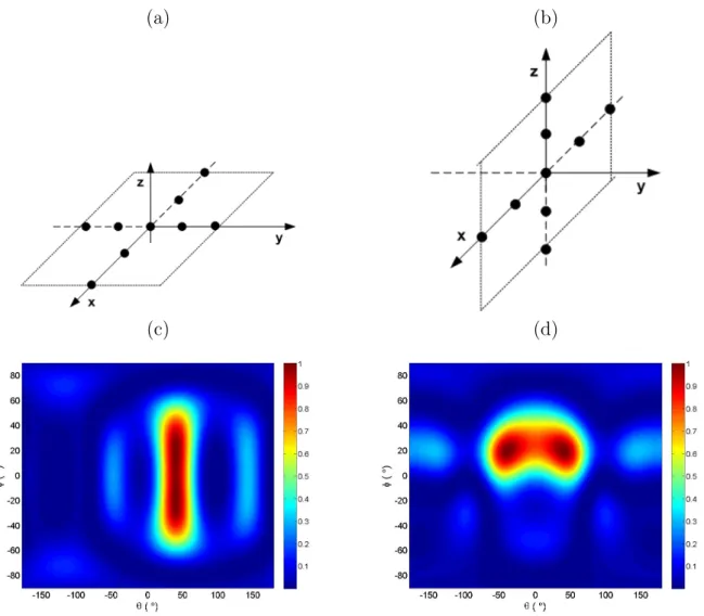
2.8 Planar array of 9 equispaced sensors with 1 m spacing, c = 1500 m/s, at frequency 500 Hz and source DOA (θs, φs) = (40◦, 20◦), for: horizontal (a)

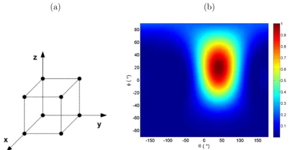
and vertical configurations (b) and the normalized beam pattern obtained for the horizontal (c) and vertical configurations (d). . . 31 2.9 Cubic array configuration of 8 equispaced sensors with 1 m spacing, c =

1500 m/s, at frequency 500 Hz and source DOA (θS, φS) = (40◦, 20◦) (a) and

the corresponding normalized beam pattern (b). . . 32 2.10 Three-dimensional representation of the beam pattern, calculated by the

beam-former considering a VSA of 9 equispaced elements with 1 m spacing, at fre-quency 500 Hz and source DOA (θs, φs) = (40◦, 20◦). . . 35

2.11 Two-dimensional normalized ambiguity surface considering a VSA of 9 eq-uispaced elements with 1 m spacing, at frequency 500 Hz and source DOA (θs, φs) = (40◦, 20◦). . . 36

(21)

3.1 Ray tangent and normal vectors esand en(a); Beam amplitude along the ray

normal direction (b). . . 42 3.2 Projection of the horizontal particle velocity vr on (x, y) axes with the

az-imuthal direction of the source, ϕs. . . 44

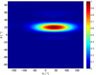
3.3 DOA estimation simulation results at frequency of 7500 Hz with azimuth θS =

45◦ and elevation φS = 30◦ angles considering: the p-only Bartlett estimator

(a), the [cos2(δ)] of Eq. 3.33) (b), the [4 cos4(δ₂)] of Eq. (3.37) (c), the particle velocity only components (v-only) or Eq. (3.33) (d) and all sensors of the VSA (p + v) or Eq. (3.37) (e). . . 55 3.4 Simulation scenario based on a typical setup encountered during the MakaiEx’05

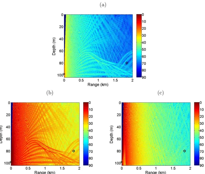
experiment with a deep mixed layer, characteristic of Hawaii. The source is bottom moored at 98 m depth and 1830 m range. The VSA is deployed with the deepest element positioned at 79.9 m. . . 56 3.5 Ray tracing calculated with TRACEO for the simulation scenario presented

in Fig. 3.4; source depth 98 m and receiver range 1830 m; the VSA is deployed with the deepest element positioned at 79.9 m. The symbol (x) indicates de position of the source and the symbol (o) indicates the position of the VSA. 58 3.6 Transmission loss calculated with TRACEO Gaussian beam model, at 13000 Hz,

for the acoustic pressure (a), horizontal particle velocity component (b) and vertical particle velocity component (c), considering the simulation scenario and the sound speed profile presented in Fig. 3.4. The symbol (x) indicates de position of the source and the symbol (o) indicates the position of the VSA. 59 3.7 Transmission loss calculated with MMPE model, at 13000 Hz, for the acoustic

pressure (a), horizontal particle velocity component (b) and vertical particle velocity component (c), considering the simulation scenario and the sound speed profile presented in Fig. 3.4. The symbol (x) indicates de position of the source and the symbol (o) indicates the position of the VSA. . . 60 3.8 Three-dimensional representation of the Bartlett estimator power for three

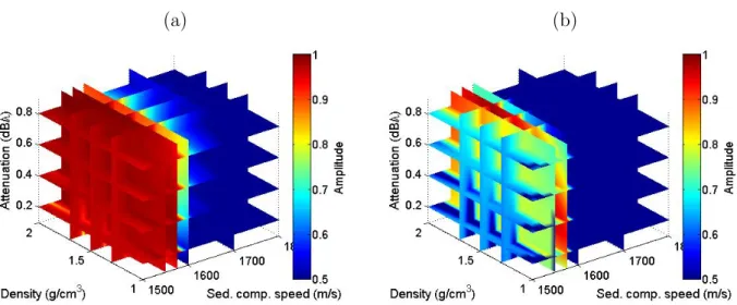
seabed parameters, at frequency 13000 Hz, considering the p-only estimator with 4 hydrophones (a) and the VSA (p + v) estimator (b). . . 63 3.9 Two-dimensional cross-sections of ambiguity surfaces estimation simulation

results, obtained with the Bartlett estimator at frequency 13000 Hz, for cp =

1575 m/s, ρ = 1.5 g/cm3 _{and α = 0.6 dB/λ considering: the p-only estimator}

(4 hydrophones) for fixed compressional attenuation (a), fixed density (b) and fixed sediment compressional speed (c) and the VSA (p + v) estimator (3.36) for fixed compressional attenuation (d), fixed density (e) and fixed sediment compressional speed (f). . . 64 3.10 One-dimensional cross section ambiguity surfaces obtained with normalized

Bartlett estimator at frequency 13000 Hz, for cp = 1575 m/s, ρ = 1.5 g/cm3

and α = 0.6 dB/λ considering the p-only estimator with 4 and 16 hydrophones and the VSA (p + v) estimator for: sediment compressional speed (a), density (b) and compressional attenuation (c). . . 66 3.11 One-dimensional cross sections ambiguity surfaces obtained with normalized

Bartlett estimator, at frequency 13000 Hz, for cp = 1575 m/s, ρ = 1.5 g/cm3

and α = 0.6 dB/λ considering the individual data components (vx, vy and vz),

v-only estimator and the VSA (p + v) estimator for: sediment compressional speed (a), density (b) and compressional attenuation (c). . . 68

(22)

XVII

3.12 Two-dimensional cross-sections ambiguity surfaces simulation results obtained with Bartlett estimator, at frequency 13000 Hz, for cp = 1575 m/s, ρ =

1.5 g/cm3 and α = 0.6 dB/λ considering the vertical particle velocity only component in Eq. (3.32) for fixed compressional attenuation (a), fixed den-sity (b) and fixed sediment compressional speed (c). . . 69 3.13 Three-dimensional representation of the vz-only Bartlett estimator power, for

the three seabed parameters, at frequency 13000 Hz, considering several slices for: compressional attenuation (a), density (b) and sediment compressional speed (c). . . 70

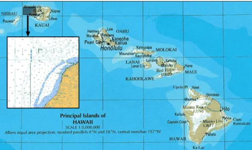
4.1 MakaiEx’05 site off the north west coast of Kauai Island, Hawaii, USA. . . . 74 4.2 Bathymetry map of the Makai experiment area and the location of the testbed

acoustic sources TB1 and TB2, thermistor strings TS2 and TS5, XBT and XCTD. . . 76 4.3 Thermistor strings temperature data in ◦C: TS2 (a) and TS5 (b) during

MakaiEx’05 sea trial, between September 17th (Julian day 260) and Septem-ber 29th (Julian day 273). . . 77 4.4 Sound speed profiles during September 20th (Julian day 264 ) and the mean

sound speed profile - black thick line. . . 78 4.5 Constitution of a single vector sensor and x, y and z-axis orientation. . . 78 4.6 A five-element vertical VSA: hose (a) and 10 cm element spacing view (b). . 79 4.7 Spectogram of noise generated by R/V Kilo Moana on VSA pressure-only

sensor at 79.6 m depth, on September 20th (Julian day 264). . . 80 4.8 Power spectrum estimates (periodogram with 1 s averaging time) of noise

gen-erated by R/V Kilo Moana on September 20th, on vector sensor at 79.6 m depth for: pressure-only sensor (a), vx component (b), vy component (c) and

vz component (d) of particle velocity sensors. . . 81

4.9 The normalized ambiguity surfaces for DOA estimation, obtained with mea-sured VSA data on September 20th at frequency 300 Hz, using the Bartlett beamformer considering: v-only (a) and VSA (p + v) (b). . . 82 4.10 Azimuth estimation results during the VSA data acquisition period at the

frequency 300 Hz on: September 20th (a), September 23rd (b) and September 25th (c). . . 83 4.11 The heading data from ship’s instruments (a) and the x and y-axis orientation

of VSA relatively to Kilo Moana’s heading, bearing in mind the ship’s noise azimuth angle estimation on September 20th. . . 84 4.12 The heading data from ship’s instruments (a), the trajectory of the R/V Kilo

Moana (green line) and the orientation of x particle velocity component of the VSA obtained from ship’s noise and ship’s heading during the drift, on September 23rd (b). . . 85 4.13 The heading data from ship’s instruments (a), the orientation of x and y-axis

of the VSA obtained from ship’s noise and ship’s heading, and the trajectory of the acoustic source Lubell 916C, on September 25th. . . 86 4.14 The bathymetry map of the MakaiEx’05 area and the position of the acoustic

sources TB1, TB2 and the VSA on September 20th - deployment 1. . . 88 4.15 The bathymetric profile between the VSA and TB1 (a) and TB2 (b) on

(23)

4.16 The 10 s received probe signals on VSA and transmitted by the acoustic sources: TB1 (a) and TB2 (b) on September 20th, constituted by LFM’s, multitones, an M-sequence and a communication signal sequence. . . 89 4.17 Source DOA estimation results obtained for frequency 8250 Hz, for: TB1 at

minute 1 where the maximum is at (127◦, 81◦) (a) and TB2 at minute 3 where the maximum is at (160◦, 95◦) (b). . . 90 4.18 The estimated azimuth results obtained for frequency 8250 Hz during the data

acquistion period, for: TB1 (blue asterisk) and TB2 (red triangle); and the ex-pected bearing obtained from the GPS data, ship’s heading and the estimated VSA horizontal plane orientation discussed in section 4.2, black asterisk for TB1 and black triangle for TB2. . . 91 4.19 Bathymetric profile during the drift (a) and source - receiver range (b) on

September 23rd - deployment 2. . . 92 4.20 The estimated azimuth results obtained for frequency 8250 Hz during the

pe-riod of data acquistion for TB2 (blue asterisk) and the expected bearing ob-tained from GPS data, ship’s heading and the estimated VSA horizontal plane orientation discussed in section 4.2 (red asterisk), on September 23rd - deploy-ment 2. . . 92 4.21 The location of VSA and the RHIB track during part of September 25th

-deployment 3. . . 93 4.22 The bathymetric profile (a) and source-receiver range (b) between VSA and

Lubell source, on September 25th - deployment 3. . . 93 4.23 The 2 minutes received signal on the VSA, transmitted by the Lubell 916C

source on September 25th, constituted by LFM’s, M-sequences and multitones in the 500-14000 Hz band. . . 94 4.24 The estimated azimuth results for the source Lubell 916C (blue asterink) with

a 90◦offset deducted (red asterisk), obtained on September 25th for frequency: 6550 Hz (a) and 9032 Hz (b) and the expected bearing from GPS data (black asterisk). . . 95

5.1 Sketch of the ray approached geometry of a plane wave emitted by an acoustic source (S) and received by a receiver (R) at the elevation angle φ0. . . 99

5.2 The location of VSA and the RHIB track during part of September 25th (deployment 3), where the source position is shown at approximately 200 m and 500 m range. . . 101 5.3 The vertical beam response at the source azimuth angle obtained using the

four p-only sensors of the VSA for minute 38 (a), 41 (b), 44 (c) and 48 (d). . 103 5.4 The vertical beam response at the source azimuth angle obtained using the

four-elements VSA for minute 38 (a), 41 (b), 44 (c) and 48 (d). . . 104 5.5 The vertical beam response at the source azimuth angle obtained using the

four individual particle velocity components of the VSA: vx-component (a)

and (b), vy-component (c) and (d), and vz-component (e) and (f). The results

where obtained for minute 38 on the left side and for minute 48 on the right side, source-range 500 m and 200 m respectively . . . 105 5.6 The bottom reflection loss at 8-14 kHz frequency band, deduced from the

down-up ratio of the experimental data on September 25th at minute 48 and 200 m source-range (a) and as modelled by the SAFARI model (b). . . 107

(24)

XIX

5.7 The bottom reflection loss at 8-14 kHz frequency band, deduced from the down-up ratio of the experimental data on September 25th at minute 38 (a) and at minute 44 (b). . . 109 5.8 The bottom reflection loss in the 8-14 kHz frequency band, deduced from the

down-up ratio of the experimental data on September 20th (deployment 1) at minute 19 (a) and at minute 27 (b). . . 110 5.9 The bathymetry map of the MakaiEx’05 area, the location of the VSA on

September 20th (deployment 1) and September 25th (deployment 3), the lo-cation of the acoustic source TB2 and the Lubell 916C trajectory. . . 111 5.10 The bathymetry map of the MakaiEx’05 area with the locations of the VSA

and the acoustic source TB2 (a) and baseline environment with the mean sound speed profile (b) on September 20th (deployment 1). The VSA was deployed with the deepest element at 79.9 m and the TB2 was bottom moored at 98 m. . . 113 5.11 Maxima of hypercube slices along time for the sediment compressional speed

at frequency 13078 Hz, considering the VSA (p + v) Bartlett estimator (a) and the vz-only Bartlett estimator (b). . . 114

5.12 The experimental data normalized ambiguity surfaces for compressional at-tenuation and density, taking into account the sediment compressional speed value of 1580 m/s, using the p-only Bartlett estimator (a), the VSA (p + v) Bartlett estimator (b) and the vz-only Bartlett estimator (c). . . 116

5.13 The experimental data normalized ambiguity surfaces using the geometric mean of estimates over time (two hours), considering: the VSA (p+v) Bartlett estimator for sediment compressional speed versus density (a) and sediment compressional speed versus attenuation (b) and the vz-only Bartlett estimator

for sediment compressional speed versus density (c) and sediment compres-sional speed versus attenuation (d). . . 117 5.14 The experimental data normalized ambiguity surfaces for sediment

compres-sional speed during data acquisition period (two hours), using : the p-only Bartlett estimator (a), the VSA (p + v) Bartlett estimator (b) and vz-only

(25)

(26)

List of Tables

4.1 Time schedule of VSA deployments during MakaiEx’05. . . 79 4.2 Geographic localization and geometric characteristics of acoustic sources, TB1

and TB2; last two columns show the estimated source depth (SD) and the estimated source range between the acoustic sources and the VSA, obtained from GPS and R/V Kilo Moana ship’s instruments. . . 87

5.1 The estimated bottom parameters taking into account the measured VSA data on September 25th and manual adjustments on SAFARI model, considering a four-layer structure. . . 109

(27)

(28)

Chapter 1 Introduction

Covering almost 75% of the planet, the ocean is a vast, complex, mostly dark world, largely

unknown and unexplored by man. Understanding the ocean and its behavior is important

to scientists in diverse areas such as oceanography, seismic exploration, weather and climate

monitoring, etc., and has barely been touched by today’s science and technology [1]. The

ocean is essentially opaque to light and electromagnetic radiation but it is transparent to

acoustic signals. Therefore, sound is the only practical way to propagate signals to great

distances in the ocean. The propagation of sound in the ocean is of vital importance, not

only for communication between marine animals but also for finding objects, measuring

water depth, currents, or other environmental parameters.

Underwater acoustics is the study of the propagation of sound in water and its interaction

with the ocean boundaries (surface and seafloor), consequently underwater acousticians use

this knowledge to predict the characteristics of physical and biological parameters of the

ocean through which it has traveled, to communicate or to find objects and intruders. As

a mechanical wave of energy, sound changes the pressure of the medium. Changes in sound

speed can be related to small changes in the average temperature of the ocean which in turn

is strongly influenced by the environmental conditions. Sound speed is an empirical function

(29)

of temperature, salinity and depth [2] and these parameters are affected not only by seasonal

and diurnal changes but also depend on the geophysical properties of the water column and

seabed [3].

Ocean acoustic tomography (OAT) is a remote sensing technique used in underwater

acoustics to study average temperatures over large regions of the ocean. It was proposed

in 1979 by Munk and Wunsch [4, 5] for global ocean monitoring. Due to interest in large

scale monitoring, OAT techniques measure the perturbation of sound travel time between

a source and a receiver at known locations to estimate sound speed disturbances, and has

been thoroughly investigated normally at low frequency (below 2 kHz), both theoretically

and experimentally [5, 6, 7].

After the cold war, due to regional conflicts in costal countries, self protection and port

entrance security, gas and oil exploration, ocean wave influence, etc., the interest in

under-water acoustics shifted to shallow under-water - say for depths less than 200 m [8]. In shallow

water, the interaction of sound with the sea surface and seabed, where it can be reflected

and transmitted into the sediments, is particularly relevant. Seabed parameters are generally

not known in sufficient detail and with enough accuracy to permit satisfactory long-range

predictions [2]. Therefore, the estimation of such parameters with sufficient resolution is

important to characterize the environment for underwater acoustic applications. A further

complication being that shallow water is usually a noisy environment affected by ship traffic

and other human activity along the costal zones.

In order to provide high estimation resolution of ocean parameters using low frequency

signals led to large aperture hydrophone arrays with many elements used to cover most of

(30)

3

as difficulties in deployment and long term operation, even in shallow water. Therefore,

the use of high-frequency (HF) signals in OAT (defined here as in the 5-50 kHz band) has

become the subject of investigation [9]. This frequency band, historically included torpedo

interception, is the subject of renewed interest related to research in acoustic

communica-tion, target scattering, HF tomography and bioacoustics. OAT with HF signals (short wave

length) can be potentially advantageous in fine resolution of ocean disturbances and seabed

parameters characterization over a particular area. Furthermore, using HF signals has

oper-ational advantages since it allows for small aperture arrays, and a single system can be used

in various acoustical applications such as source localization, underwater communications

and geoacoustic inversion.

Recent developments in new piezoelectric materials (PMN-PT crystals) and new

elec-tromechanical design have led to a new generation of sensors - the vector sensors [10]. Each

vector sensor is constituted by one omni-directional hydrophone and three uni-axial

ac-celerometers. The omni-directional hydrophone is sensitive to the acoustic pressure, in the

following termed as acoustic pressure-only; each accelerometer is sensitive to the acoustic

particle velocity only along a specific axis while being very insensitive in the other two axes,

in the following termed as particle velocity components. Therefore, a vector sensor is able to

measure both the acoustic pressure and the three particle velocity components providing the

directional capabilities of the sensor. A crucial advantage of vector sensors over hydrophones

is the quantity of information obtained from a single point spatial device. The spatial

filter-ing capabilities of vector sensors have become a subject of investigation, predominantely in

direction of arrival (DOA) estimation [11, 12, 13, 14]. The potential gain verified in DOA

(31)

allow for high performance small aperture Vector Sensor Arrays (hereafter VSA). Taking

advantage of its directionality and its performance in DOA estimation, the proposal of this

work is to estimate geoacoustic and geometric parameters with a VSA of a few elements,

to provide better estimation resolution than equivalent arrays of hydrophones (with same

number of elements). The ability of a vector sensor to measure signals in one direction while

ignoring possible noise sources from other directions can be useful to improve the estimation

of ocean parameters. Additionally, it is intended to use HF signals, consequently a VSA

can be very compact and easy-to-deploy, providing a good alternative to be embarked on

reduced dimension autonomous platforms or vehicles where space is very limited.

1.1 State of the Art

Acoustic sensor array signal processing is an active area of research, whose objective is to

estimate relevant spatial parameters such as the number of emitting sources and their

loca-tions - range, depth and DOA, through the analysis of the data collected at several sensors.

H. Krim and M. Viberg [15] discussed and summarized many of the parameter estimation

methods in sensor array processing. First of all, a signal processing technique known as

beamforming where the objective is to estimate the signal DOA. The signals from different

sensors are delayed, weighted and summed in order to create a pattern whose maximum gives

the true source DOA estimate. Beamforming techniques can be classified in two categories,

depending on how the weights are chosen: data independent (or conventional beamformers)

and statistically optimal [16]. Conventional beamformers use a fixed set of weights

inde-pendent of the array data (only the information about the location of the sensors in space

(32)

interfer-1.1. STATE OF THE ART 5

ence scenarios. In contrast, in statistically optimal beamformers the weights are selected

based on the statistics of the array data; such selection automatically optimizes the array

response according to given criteria. Multiple Sidelobe Canceller (MSC), Reference Signal,

Maximization of Signal to Noise Ratio (Max SNR) and Linearly Constrained Minimum

Vari-ance (LCMV) are different approaches of implementing optimum beamformers. However,

the statistics of the array data are usually unknown and may change with time, so adaptive

algorithms such as Least Mean Squares (LMS) or Recursive Least Square (RLS) are used to

determine weights that converge to the statistically optimal solution [16].

Beamforming was extended to the estimation of other parameters and a generalized

beamformer was introduced by Hinich [17] and Bucker [18] as a source localization method

- Matched-Field Processing (MFP). MFP consists of correlating the measured signal at the

sensors with the modelled replica field, in order to obtain the parameter that gives the

high-est correlation, which in fact is the parameter high-estimate. Hinich was the first to examine

source localization, using the spatial complexity of the underwater acoustic field to localize

the source (in range and depth) with a vertical array, but Bucker was credited with the

formulation of MFP, using realistic environmental models and introducing the concept of

ambiguity surfaces. Since this technique is a simple correlator, the most widely used

proces-sor is the Bartlett procesproces-sor, which directly correlates the measured data with the modelled

replica data. The accuracy of range and depth estimation in conventional MFP depends on

the accurate knowledge of the ocean environmental parameters. To overcome this stringent

requirement several methods were introduced. Yang [19] proposed a method of range and

depth estimation based on modal decomposition, where the reflection/scattering loss

(33)

required. The author estimated range and depth, either separately or simultaneously, by

decomposing the array data and beamforming on the mode amplitudes. The normal mode

amplitudes were used for source depth estimation while the phase differences between the

normal modes were used to source range estimation. This method was successfully applied

for data acquired during the 1982 FRAM IV experiment in the Arctic Ocean. Another

source localization method, which eliminates the need of an accurate knowledge of the ocean

environmental parameters by including these parameters in the search space, was introduced

by M. Collins in 1991 [20], namely Focalization. Focalization is a method where both the

source parameters and the environmental parameters are unknown or partially unknown.

The environmental parameters are adjusted in an attempt to localize the acoustic sources,

i.e., simultaneously focus and localizes. But if MFP is sensitive to the environmental

infor-mation and if the source locations are known or partially known, this technique can also be

used to invert the environmental parameters. This concept has demonstrated an increased

interest in underwater acoustics relating to a wide range of inversion problems - generically

called Matched-Field Inversion (MFI) [21]. However, a first work suggesting that MFP could

be used to environmental parameters was presented in 1987 by A. Tolstoy in [22]. The

au-thor examined the estimation of rms surface roughness for a known source with simulated

data. Then, applications of MFI were suggested for tomography, where the estimation of

deep water sound speed profiles was first proposed in [23] and later extended in [24] for the

estimation of geoacoustic profiles in shallow water environments.

Thus, the 90s saw the beginning of the use of the MFP concept for environmental

inver-sion. In particular, geoacoustic inversion based on MFI techniques is a research area that

(34)

1.1. STATE OF THE ART 7

intrusive remote sensing technique of great importance, since the geoacoustic properties such

as sediment layer thickness, sediment sound speed profiles, density and attenuation, can be

rapidly and efficiently estimated; in contrast with direct measurements, which are difficult

and almost impossible to survey any region extensively [21]. In fact, assessing seabed

pa-rameters with in situ measurements such as grabs and cores [25], is an expensive task and

time consuming process and only a limited area, where the measurements are collected, is

characterized. In [26] properties of the ocean bottom were estimated using the concepts of

MFI. The inversion method was illustrated for seabed parameters (sound speed, density,

at-tenuation and layer thickness) in a range independent environment and for bathymetry and

bottom sound speed in a range dependent environment. However, the number of parameters

to be estimated can be extremely large and an exhaustive search of the optimal solution

could be very difficult. Thus, with the development of numerical models and the increase of

computer power, the inversion of the geoacoustic parameters can be posed as an optimization

problem using techniques, such as genetic algorithms [27, 28], simulated annealing [29, 30]

or even based on a Bayesian formulation [31] to address a large number of parameters over

a wide parameter search space.

In the implementation of those inversion methods is common to use vertical arrays of

hydrophones to cover almost all the water column. In order to simplify the array systems

and to create easier deployment and lower cost systems, research involving different array

configurations suggested that it is possible to estimate seabed parameters from data

ac-quired by horizontal hydrophone arrays, which could be towed [32, 33] or bottom moored

[34]. Furthermore, in [35] it was proposed and tested with experimental results a geoacoustic

(35)

demon-strated that a single transmission of a broadband (200-800 Hz) coded signal received at a

single depth was sufficient to correctly estimate bottom properties. The results were

com-pared with MFP of multitone data received on a vertical hydrophone array showing good

agreement. Other experimental results of acoustic inversion methods with broadband signals

and short aperture arrays were presented in [36].

At this point, it should be remarked that geoacoustic inversion is not only based on

methods where the measured data is directly correlated with the modelled data to estimate

the parameters of interest. The inversion of seabed parameters could also be obtained from

measurements of the reflection coefficient as a function of the angle of incidence (or grazing

angle). The technique takes advantage of the fact that the reflection loss at the

water-sediment interface and, sound speed and attenuation profiles in the water-sediment influence the

acoustic propagation. An inversion process based on the Biot’s theory context is presented

in [37], where the sensitivity of the reflection coefficient due to the geophysical properties

(such as porosity, grain density, permeability, pore size, etc.) were discussed. Another

method for estimating the elastic properties of the seafloor sediment, based on the reflection

amplitude measurements from explosive charges, is described in [38]. This work noticed that

the relationship between the signal amplitude and the angle of incidence can be described by

the reflection coefficient, which was calculated for different values of density, compressional

and shear-wave speeds. Another method of geoacoustic inversion based on the reflection loss

estimation was proposed by C. Harrison et al. in [39]. The method consists on the extraction

of the reflection loss from the vertical array measurements of ambient noise, such as surface

generated noise in the 200-1500 Hz band. The method uses experimental data acquired on

(36)

extended in [40] to 1-4 kHz using an array of 32 elements at 0.18 m spacing and length of

5.58 m. The ratio between downward and upward beam responses is an approximation of

the bottom reflection coefficient, and the reflection loss versus angle is directly found by

comparing the noise intensity arriving from equal down and up elevation angles. Then,

comparisons between measurements and predictions provide the number of layers, their

thickness and the respective bottom parameters. This technique will be described in more

detail in Chapter 5.

The previously described techniques have been applied using acoustic pressure signals

acquired by omni-directional hydrophones, which sense the acoustic pressure equally in every

direction. Since the 1980s, the idea of measuring particle velocity beyond the acoustic

pressure field appeared in underwater acoustics to improve the DOA estimation. The U.S.

Navy has been using a DIFAR (DIrectional Frequency Analysis and Recording) sonobuoy to

detect submarines, using two horizontal particle velocity components as well as the pressure.

The horizontal particle velocity allows to determine the azimuth of low frequency sounds

below 2 kHz. The DIFAR concept was only used for scientific purposes in the 90s [41], where

a vertical line array of DIFAR sensors was designed and constructed by the Marine Physical

Laboratory’s. The main features of this DIFAR array were described in [42], where each

element consisted of three orthogonally-oriented geophones to measure the corresponding

particle velocity components and a hydrophone to measure the acoustic pressure. The array

was constituted by 16 sensor elements, with 15 m spacing between elements, in the

10-270 Hz band; each element had a compass to measure the orientation of the two horizontal

geophones with respect to magnetic North. The concept of acquiring the particle velocity

(37)

hydrophones are used. D’Spain et al. in [43] presented beamforming results with data

collected from the first sea test of a DIFAR array. The DOA estimation results for a towed

source, using conventional and adaptive beamforming methods, provided surprisingly good

spatial resolution in azimuth estimation, in addition to the vertical resolution of the array’s

225 m aperture.

The use of directional sensors becomes a subject of investigation, where several authors

have been conducting research on theoretical aspects of vector sensor processing, initially

for air [44, 45] and then extended for underwater acoustics [11, 12, 13]. Tabrikian et al.

[44] proposed an efficient electromagnetic vector sensor configuration for source localization

in air. The authors found that the minimum number of sensors, capable of estimating the

DOA of an arbitrary polarized signal from any direction, is two electric and two magnetic

sensors referred to as quadrature vector sensor. Nehorai and Paldi developed an analytical

model, initially for electromagnetic sources [45], and then extended it to the underwater

acoustic case [11], where an ideal vector sensor, consisting of one omni-directional pressure

sensor and three particle velocity-meters that are sensitive in a specific direction (x, y or

z), was considered. The performance of a VSA was compared to that of a hydrophone

array for DOA estimation and it was suggested that this type of device has the ability to

provide directional information, with a clear advantage in DOA estimation and gives rise to

an improved accuracy. The authors also derived a compact expression for the Cram´er-Rao

Lower Bound (CRLB) on the estimation errors of the source DOA. Thus, the vector sensors

emerged as a potential competitor to traditional omni-directional hydrophones. Cray and

Nuttall [12] applied the plane-wave beamforming to particle velocity sensors and compared

(38)

directivity gain not possible to achieve with an equivalent number of hydrophones. Wan et al.

[13] performed a comparative simulation study of DOA estimation using classic methods such

as MUltiple SIgnal Classification (MUSIC) and Minimum Variance Distortionless Response

(MVDR) estimators, with vector sensors, gradient sensors and pressure sensors. The results

show that VSAs outperform gradient hydrophone arrays, which consist of three pressure

hydrophones symmetrically mounted in a circle.

Recently, theoretical work using quaternion based algorithms has been proposed for

pro-cessing VSA data for DOA estimation [46, 47, 48]. Quaternions are a four dimensional

hypercomplex number representation, where each quaternion is described by four

compo-nents: one real and three imaginary numbers. In [46, 47, 48], the real part was attributed to

the acoustic pressure and the imaginary part to the three particle velocity components. The

authors proposed a quaternion based MUSIC algorithm (Q-MUSIC) for DOA and

polariza-tion parameter estimapolariza-tion. The results were compared to the classical MUSIC algorithm

for scalar sensor array and to another MUSIC-like algorithm for VSA (V-MUSIC). It was

shown that Q-MUSIC is clearly more accurate than classical MUSIC and presents equivalent

results when compared to V-MUSIC; the Q-MUSIC reduces the computational memory

re-quirements for covariance matrix estimation, which may be relevant for specific applications.

Since 2006, research involving experimental VSA data appeared in the scientific literature.

Lindwall [49] showed the advantage of using vector data over scalar data for image structures

in a 3-D volume. This was supported by a scale experiment with a vector sensor in a water

tank. The author used the same type of vector sensor considered in this thesis, which was

specially designed for use in water by the Naval Underwater Warfare Center in collaboration

(39)

provide directional information on target noise sources. Shipps and Abraham [10] described

the new vector sensor developed for the U.S. Navy, which can be particularly useful in

underwater acoustic surveillance and port security. VSAs can improve the detection or

localization of acoustic signals compared with hydrophone arrays and have the ability, for

example, to detect acoustic signals from an intruder that are quieter than the surrounding

noise sources, which can not be detected by a hydrophone array [10]. The VSA is able to

estimate both elevation and azimuth angles, eliminates the well known left/right ambiguity of

linear arrays and provides better resolution than hydrophone arrays. The crucial advantage

of VSA verified in three dimensional DOA estimation can be potentially applied to the

estimation of other geometric or environmental parameters. Therefore, applications of the

VSA appear in underwater communications [50, 51] and geoacoustic inversion [52]. The

results presented in [50, 51] suggest that a single vector sensor has better performance than

a single pressure sensor or even pressure-only arrays. It was found that a single vector sensor

improves significantly the signal-to-noise ratio (SNR) when compared with pressure-only

arrays. The usefulness of particle velocity information in underwater communications was

demonstrated and the vector sensor can offer an attractive acoustic communication solution

for compact underwater platforms and underwater autonomous vehicles, where space is very

limited. A geoacoustic inversion scheme based on experimental data measured by a VSA

using low frequency signals (central frequency 400 Hz), was proposed by Peng and Li [52].

The authors showed that the vector sensor can reduce the uncertainty on the estimation of

the sediment compressional speed.

High-frequency acoustics is another, albeit unexpected, emerging research topic [8]. HF

(40)

of high attenuation in the ocean volume. Moreover, the propagation of short wave length

(HF) signals is highly influenced by bottom and surface scattering, hence difficult to model.

However, for surprise of many, the sound energy is not annihilated by contact with boundaries

and it can reflect many times and still yield distinct echoes [53]. Some theoretical and

experimental works proved that environmental properties can be characterized using HF

signals [40, 54, 55]. A pioneer work in HF tomography was presented by Lewis et al. [9].

This work revealed that arrival times between source-receivers at short distances (3-5 km) at

frequencies in the 8-11 kHz band were readily detectable and distinguishable. Furthermore,

the use of HF signals provides [53, 55]:

1. The use of small aperture arrays due to short wave length;

2. The use of small sources to emit the signals;

3. A fine resolution of ocean variations in Ocean Acoustic Tomography and Matched-field

Processing applications;

4. The characterization of bottom parameters in a particular area.

Additionally, the usage of HF signals in underwater acoustic communications is important,

since a high bandwidth is required in order to transmit a higher data rate. In [51] a time

reversal multichannel receiver was proposed to exploit the use of particle velocity information

for underwater acoustic communications, using experimental data acquired during Makai

experiment 2005. The authors compared the results of a single vector sensor with a

pressure-only sensor array in HF band. Such results show that the vector sensor, besides a significant

(41)

with the VSA can be advantageous to increase the resolution of ocean parameters estimation

and to reduce the array’s aperture, providing more portable and compact systems to be used

in underwater acoustics applications.

The present work addresses the above mentioned subjects aiming to contribute to the

development of more efficient acoustic remote sampling systems. A particle velocity-pressure

joint data model (VSA data model) and a VSA-based Bartlett estimator are proposed, in

order to demonstrate the capabilities of using a VSA in ocean parameter estimation. The

highlighted advantages of the VSA-based Bartlett estimator over pressure-only estimator will

be tested for DOA estimation using low and HF signals, and most importantly for seabed

parameter estimation using HF signals.

1.2 Work motivation and Contributions

Traditionally, source localization - range, depth and DOA - and the estimation of other

pa-rameters such as ocean bottom papa-rameters, are found using low frequency signals and long

hydrophone arrays, in order to get as higher estimation resolution as possible. In fact, long

hydrophone arrays are not a practical solution to be embarked on reduced dimension

au-tonomous moving platforms or vehicles where space is limited. During the last two decades,

the use of directional sensors captured the attention of the scientific community; vector

sensor arrays were designed in order to outperform traditional hydrophone arrays in DOA

estimation. In fact, vector sensors have the ability to provide directional information

be-cause they measure the components of particle velocity along each spatial direction. The

high directivity of a single vector sensor allows a VSA to emerge as a potential alternative

(42)

1.2. WORK MOTIVATION AND CONTRIBUTIONS 15

Most of the research involving vector sensors is related to DOA estimation in a simulation

context, or using low frequency signals; in both cases it was shown the feasibility of vector

sensors for DOA estimation and it was also shown that vector sensors exhibit an improved

performance over pressure-only sensors. From such studies the following questions arise:

• What are the common and differentiating features of the particle velocity field when compared to the pressure field?

• Why does the VSA performance increase when compared with equivalent hydrophone arrays?

• Can the high directivity of the VSA be used with advantage for the estimation of other ocean parameters such as water column temperature or seabed parameters?

• Can the potential gain of the VSA be extended to three-dimensional source localization and geoacoustic inversion using a small aperture VSA, acquiring HF signals?

• How is the sensitivity of each particle velocity component to a particular environmental parameter?

The main objective of the present work is to answer these questions (and additional

others) along the discussion presented in the following sections. To such end, standard

estimation techniques were extended in order to account for particle velocity, and extensive

tests were performed based on simulations and on the processing of experimental data. On

the basis of the obtained results the following contributions can be highlighted:

• A particle velocity-pressure joint data model - VSA data model - is derived, taking into account the relationship of the particle velocity with the acoustic pressure from

(43)

the linear acoustic equation (Euler’s equation). The VSA data model is based on a ray

physical description, using the Gaussian beam approximation of the ray pressure [56];

• An estimator based on an extension of the conventional pressure-only Bartlett estima-tor including particle velocity information is proposed. Two VSA-based Bartlett

esti-mators are derived for generic ocean parameter estimation, bearing in mind the VSA

data model with and without the acoustic pressure. The performance of the VSA-based

Bartlett estimators relative to the pressure-only Bartlett estimator is analytically

de-duced, clearly showing the advantages of the VSA over pressure-only sensors. It will

be seen that the VSA-based Bartlett estimators are proportional to the pressure-only

Bartlett estimator, where the terms of proportionality are given by a directivity factor.

Such directivity factor is the crucial advantage of using particle velocity information

in underwater acoustic estimations, providing an improved sidelobe reduction or even

supression and increasing the estimation resolution of the ocean parameters;

• The proposed VSA-based Bartlett estimators are tested, with simulated and exper-imental data, for DOA estimation and for geoacoustic inversion. The experexper-imental

data considered in this work was acquired by a four-element vertical VSA in the

100-14000 Hz band during Makai experiment 2005 (MakaiEx’05). The MakaiEx’05 was

or-ganized by HLS Research and was designed to bring together a number of researchers

with interests in different aspects of HF acoustics (acoustic communications, target

scattering, HF tomography, etc.). This experiment was conducted from 15 September

to 2 October, 2005, off Kauai Island, Hawaii (USA) [55];