Inverse modeling of hydrologic parameters using surface flux and runoff observations in the Community Land Model

(1)

HESSD

10, 5077–5119, 2013

Inverse modeling of hydrologic parameters

Y. Sun et al.

Title Page

Abstract Introduction

Conclusions References

Tables Figures

◭ ◮

Back Close

Full Screen / Esc

Printer-friendly Version Interactive Discussion

Discussion

P

a

per

|

Dis

cussion

P

a

per

|

Discussion

P

a

per

|

Discussio

n

P

a

per

Hydrol. Earth Syst. Sci. Discuss., 10, 5077–5119, 2013 www.hydrol-earth-syst-sci-discuss.net/10/5077/2013/ doi:10.5194/hessd-10-5077-2013

Geoscientiic Geoscientiic

Hydrology and Earth System

Sciences

Open Access

Discussions

This discussion paper is/has been under review for the journal Hydrology and Earth System Sciences (HESS). Please refer to the corresponding final paper in HESS if available.

Inverse modeling of hydrologic

parameters using surface flux and runo

_ff

observations in the Community Land

Model

Y. Sun1,2, Z. Hou1, M. Huang1, F. Tian2, and L. R. Leung1

1

Pacific Northwest National Laboratory, P.O. Box 999, Richland, WA 99352, USA

2

Department of Hydraulic Engineering, State Key Laboratory of Hydroscience and Engineering, Tsinghua University, Beijing 100084, China

Received: 1 April 2013 – Accepted: 13 April 2013 – Published: 23 April 2013 Correspondence to: Z. Hou (zhangshuan.hou@pnnl.gov)

(2)

HESSD

10, 5077–5119, 2013

Y. Sun et al.

Title Page

Tables Figures

◭ ◮

Back Close

Full Screen / Esc

Discussion

P

a

per

|

Dis

cussion

P

a

per

|

Discussion

P

a

per

|

Discussio

n

P

a

per

|

Abstract

This study demonstrates the possibility of inverting hydrologic parameters using

sur-face flux and runoffobservations in version 4 of the Community Land Model (CLM4).

Previous studies showed that surface flux and runoffcalculations are sensitive to major

hydrologic parameters in CLM4 over different watersheds, and illustrated the

neces-5

sity and possibility of parameter calibration. Two inversion strategies, the deterministic least-square fitting and stochastic Markov-Chain Monte-Carlo (MCMC) Bayesian in-version approaches, are evaluated by applying them to CLM4 at selected sites. The

unknowns to be estimated include surface and subsurface runoff generation

param-eters and vadose zone soil water paramparam-eters. We find that using model paramparam-eters

10

calibrated by the least-square fitting provides little improvements in the model simula-tions but the sampling-based stochastic inversion approaches are consistent – as more information comes in, the predictive intervals of the calibrated parameters become nar-rower and the misfits between the calculated and observed responses decrease. In general, parameters that are identified to be significant through sensitivity analyses

15

and statistical tests are better calibrated than those with weak or nonlinear impacts on

flux or runoffobservations. Temporal resolution of observations has larger impacts on

the results of inverse modeling using heat flux data than runoffdata. Soil and vegetation

cover have important impacts on parameter sensitivities, leading to different patterns

of posterior distributions of parameters at different sites. Overall, the MCMC-Bayesian

20

inversion approach effectively and reliably improves the simulation of CLM under diff

er-ent climates and environmer-ental conditions. Bayesian model averaging of the posterior

estimates with different reference acceptance probabilities can smooth the posterior

distribution and provide more reliable parameter estimates, but at the expense of wider uncertainty bounds.

(3)

HESSD

10, 5077–5119, 2013

Y. Sun et al.

Title Page

Tables Figures

◭ ◮

Back Close

Full Screen / Esc

Discussion

P

a

per

|

Dis

cussion

P

a

per

|

Discussion

P

a

per

|

Discussio

n

P

a

per

1 Introduction

Inverse problems (or parameter calibrations/optimizations) involve a general framework to derive from measurements information about a physical object or system (Taran-tola, 2005). During the past decades, numerous inversion strategies, deterministic or stochastic, have been developed and applied in earth systems sciences including

at-5

mospheric science, hydrology, geology, and geophysics. Three conditions (existence, uniqueness, stability of the solutions) are necessary for a well-posed inverse problem (Hadamard, 1902). However, as the conditions are usually violated in practice, some regularization is generally needed to introduce mild assumptions on the solution and prevent parametric over-fitting. It is also important for an inverse approach to be

capa-10

ble of quantifying and evaluating the prediction uncertainty.

For a given inverse problem, one can choose different approaches depending on the

requirements of parameter estimation accuracy, computational demand, and impor-tance of prediction uncertainty (e.g. Hou et al., 2006; Chen et al., 2004; Hoversten et al., 2006), which requires understanding of the advantages, disadvantages, and

appli-15

cability of each method. Deterministic approaches have been used to obtain ‘optimal’ parameter sets by evaluating the goodness of fit between observed and model simu-lated response variables (e.g. Sorooshian, 1981; Sorooshian and Dracup, 1980; Duan et al., 1992; Duan et al., 1993; Sorooshian et al., 1993; Hoversten et al., 2006). These approaches generally assume that an optimal parameter set exists and implicitly ignore

20

the estimation of predictive uncertainties. However, a single optimal parameter set may not exist and the uncertainties associated with the optimal parameter sets could be large (e.g. Gupta et al., 1998; Klepper et al., 1991; Van Straten and Keesman, 1991; Beven and Binley, 1992; Yapo et al., 1996). Moreover, a model with the optimal param-eter set may provide the best fit over the calibration period, but multiple paramparam-eter sets

25

(4)

HESSD

10, 5077–5119, 2013

Y. Sun et al.

Title Page

Tables Figures

◭ ◮

Back Close

Full Screen / Esc

Discussion

P

a

per

|

Dis

cussion

P

a

per

|

Discussion

P

a

per

|

Discussio

n

P

a

per

|

can address these limitations by describing the input and output uncertainties in a statistical manner. Generally, the input parameter space is represented in a form of multivariate probability distributions of input parameters and must be sampled to gen-erate multiple realizations of the model simulations so that the prediction range can be estimated based on the ensemble model simulations (Beven and Binley, 1992; Freer et

5

al., 1996; Kuczera and Parent, 1998; Vrugt et al., 2003b). When multiple types of data are available, multi-objective calibration can be used to deal with parameter estimation uncertainty by combining several measures of performance for data fusion (Boyle et al.,

2000; Kollat et al., 2012; Gupta et al., 1998; Vrugt et al., 2003a). In practice, different

optimization methods can also be combined to improve the treatment of uncertainty in

10

hydrologic modeling (Vrugt and Robinson, 2007; Feyen et al., 2007; Vrugt et al., 2005). In previous studies (Hou et al., 2012; Huang et al., 2013), we investigated the

sen-sitivity of surface fluxes and runoff simulations to major hydrologic parameters in

ver-sion 4 of the Community Land Model (CLM4) by integrating CLM4 with a stochastic exploratory sensitivity analysis framework at 13 flux towers from the Ameriflux

net-15

work and 20 watersheds from the Model Parameter Estimation Experiment (MOPEX) (Huang et al., 2013) spanning a wide range of climate, landscape, and soil conditions. We found that the CLM4 simulated latent heat flux (LH), sensible heat flux (SH), and

runoffshow the largest sensitivity to subsurface runoffgeneration parameters. These

studies demonstrated the necessity and possibility of parameter inversion/calibration

20

using available measurements of surface fluxes and streamflow to invert the optimal parameter set, and provided guidance on reduction of parameter set dimensionality and parameter calibration framework design for CLM4.

This study aims to demonstrate the inversion methodology at selected sites based on the global sensitivity analyses detailed in Hou et al. (2012) and Huang et al. (2013).

25

Among various inversion approaches, we adopt and compare the performances of two

different inversion strategies, including deterministic least-square fitting and a

(5)

HESSD

10, 5077–5119, 2013

Y. Sun et al.

Title Page

Tables Figures

◭ ◮

Back Close

Full Screen / Esc

Discussion

P

a

per

|

Dis

cussion

P

a

per

|

Discussion

P

a

per

|

Discussio

n

P

a

per

subsurface runoffgeneration and vadose zone soil water movement. Different options

for the inversion framework are evaluated at the selected sites. For example, it is impor-tant to evaluate the prior incompatibility issues in an inversion design (Hou and Rubin, 2005). As detailed in the remaining sections of this paper, we evaluated the impacts of prior information (e.g., initial guesses) on the inversion results. We also compared the

5

consistency and reliability of inversion using both monthly and daily flux observations, and compared the performance of Bayesian model averaging to the individual inver-sion approaches for parameter estimation. We also discuss the issues related to data quality, data worth, and redundancy.

2 Site and data description

10

We perform parameter estimation at two flux tower sites and one MOPEX basin. The MOPEX basin is in close proximity to one of the flux tower sites to investigate model

inversion using heat flux versus runoffdata. These sites/basins are chosen based on

previous sensitivity analyses over a larger set of flux tower sites and MOPEX basins (Hou et al., 2012; Huang et al., 2013) that demonstrated the feasibility and necessity of

15

parameter calibration at those locations and to provide representative and contrasting climate and environmental conditions within the United States for more robust con-clusions. US-ARM is located in Oklahoma and is covered by croplands (Allison et al., 2005; Baer et al., 2002; Fischer et al., 2007; Riley et al., 2009; Suyker and Verma, 2009). US-MOz is located in Missouri and is covered by deciduous broadleaf (Gu et

20

al., 2012, 2006). Meteorological forcing, site information such as soil texture, vege-tation cover, and satellite-derived phenology, as well as validation datasets, such as water and energy fluxes, are provided by the North American Carbon Program (NACP) site synthesis team. The site information is provided in Table 2 in (Hou et al., 2012). MOPEX basin (07147800) is the Walnut River basin in Kansas with a drainage area

25

(6)

HESSD

10, 5077–5119, 2013

Y. Sun et al.

Title Page

Tables Figures

◭ ◮

Back Close

Full Screen / Esc

Discussion

P

a

per

|

Dis

cussion

P

a

per

|

Discussion

P

a

per

|

Discussio

n

P

a

per

|

(Ke et al., 2012). The meteorological forcing for the MOPEX basin was extracted from the phase two North America Land Data Assimilation System (NLDAS2) forcing at an hourly time step from 1979–2007 (Xia et al., 2012), including precipitation, shortwave and longwave radiation, air temperature, humidity and wind speed at a 1/8th degree resolution derived from the 32 km resolution 3 hourly North American Regional

Re-5

analysis (NARR) following the algorithms detailed in Cosgrove et al. (2003). An area-average algorithm was then applied to the NLDAS2 forcing as inputs to CLM by treating the entire basin as a single computational unit. CLM was spun up by cycling the forcing at each site for at least five times until all the state variables reached equilibrium before any statistics were calibrated for inversion, based on the methodology described below.

10

3 Methodology

3.1 Parameterization

Observational data used in parameter estimation are observed latent heat fluxes and

runoffmeasurements, which are processed and gap-filled to obtain daily and monthly

averaged data. For unknowns, we focus on the parameters that are most identifiable

15

from the response variables (i.e. they have significant, straightforward, and

distinguish-able influences on hydrologic processes, including soil hydrology and runoff

genera-tion processes). The 10 hydrologic parameters that we found to have impacts on the

simulations of surface and subsurface runoff, latent and sensible heat fluxes, and soil

moisture in CLM4 arefmax,Cs,fover,fdrai,Qdm,Sy,b,Ψs,Ks, and θs. Explanations of

20

the 10 parameters and their prior information are shown in Table 1.

3.2 Parameter calibration using least-square fitting approaches

Different approaches can be used to calibrate the selected hydrologic parameters

(7)

HESSD

10, 5077–5119, 2013

Y. Sun et al.

Title Page

Tables Figures

◭ ◮

Back Close

Full Screen / Esc

Discussion

P

a

per

|

Dis

cussion

P

a

per

|

Discussion

P

a

per

|

Discussio

n

P

a

per

squares is a standard approach to approximate the solution of over-determined sys-tems, i.e., systems specified by more equations than unknowns. One well-known ap-proach utilizing the least-square fitting concept is PEST (Parameter ESTimation) (Do-herty, 2008), which is a general-purpose, model-independent, parameter estimation and model predictive uncertainty analysis package. Here we adopt PEST to perform

5

single-objective least-square fitting of the observational data, with the loss function

de-fined as the sum square of fitted residuals between calculated and observed runoffor

latent heat fluxes. However, simulations of heat flux and runoffusing the calibrated

rameters show only small improvements compared to simulations using the default pa-rameter values. To further explore the usefulness of the least-square fitting approach,

10

the PEST-calibrated parameter estimates are used as one of the choices for initial guesses of the parameters for stochastic Bayesian updating as explained below to determine if such estimates may improve the convergence rate or robustness of the inversion results.

3.3 Bayesian updating

15

In practice, it is critical to evaluate and quantify the uncertainty associated with pa-rameter estimation; therefore, we should consider stochastic inversion/calibration ap-proaches (e.g. Bayesian inference) and describe the input/output uncertainties in a probabilistic manner. Bayesian inference derives the posterior probability as a conse-quence of two antecedents: a prior probability given prior information, and a “likelihood

20

function” derived from a probability model for the data to be observed. Bayesian infer-ence computes the posterior probability according to Bayes’ rule:

f m_|d,I

∝f d_|m,I

·f m_|I

, (1)

wheref m_|d,I

represents the posterior pdf of parameter m, f d_|m,I

denotes the

likelihood of observing d given parameter m, and f m|I is the prior pdf of m given

(8)

HESSD

10, 5077–5119, 2013

Y. Sun et al.

Title Page

Tables Figures

◭ ◮

Back Close

Full Screen / Esc

Discussion

P

a

per

|

Dis

cussion

P

a

per

|

Discussion

P

a

per

|

Discussio

n

P

a

per

|

We assume that the forward models (e.g. CLM4) are being characterized by d_{i j}∗ =

gi j(m)+εi j, where m represents the vector of model parameters, di j=gi j( ) is the

forward model, ε_{i j} is the difference (i.e. residual) between the model d_{i j} and

obser-vationd_{i j}∗ (i.e. residuals),i=1,. . .,K;j=1,. . .,Ni,K being the number of data types

and Ni being the number of observations for the i-th data type. With the underlying

5

assumptions thatεi jεi j are normally distributed with varianceσ

2

i j, and the distributions

are independent, the likelihood function can be represented as (Hou et al., 2006):

fD_|M,Σ,I(d∗_|m,σ,I)=

YK

i=1

YNi

j=1



 1

√

2πσ_{i j}exp







− 1

2σ_{i j}2

h

d_{i j}∗ ₋gi j(m)

i2 



 

. (2)

The posterior distributions of the input parameters are the products of the priors and the likelihood functions. As more information comes in, Bayes’ rule can be applied

10

iteratively, that is, after observing some evidence, the resulting posterior probability can be treated as a prior probability, and a new posterior probability is computed from the new evidence.

3.4 Sampling methods

An efficient sampling approach is important for the success of Bayesian inversion,

15

especially when the forward modeling computational demand is high, the parameter dimensionality is high, or the parameters are weakly identifiable. In this study, the Metropolis-Hasting sampling method is used to draw samples from the joint posterior distribution functions. The procedure is as follows:

(a) initialize a random vectormfrom the prior distributions{m(0)_i ,i=1,. . .,n};

20

(b) generate a random variable m∗_i,i =1,. . .,n from the proposal distributions, and

(9)

HESSD

10, 5077–5119, 2013

Y. Sun et al.

Title Page

Tables Figures

◭ ◮

Back Close

Full Screen / Esc

Discussion

P

a

per

|

Dis

cussion

P

a

per

|

Discussion

P

a

per

|

Discussio

n

P

a

per

using Eq. 2):

α=min 

pra,

prob(m∗_i_|m(1)₁ ,m(1)₂ ,. . .,m(1)_i −1,m

(0) i+1,m

(0)

i+2,. . .,m (0) p )

prob(m(0)_i _|m(1)₁ ,m(1)₂ ,. . .,m(1)_i −1,m

(0) i+1,m

(0)

i+2,. . .,m (0) p )



; (3)

(c) generate a random valueuuniformly from interval (0,1);

(d) ifα > u, letm(1)_i =m_i∗; otherwise, letm(1)_i =m(0)_i .

Repeating steps (b) to (d) by replacing index (k) with index (k+1), we can obtain many

5

samples as follows:n(m(_ik)) :i =1,. . .,n, k=0, 1,. . .,qo. From the procedure, we can

see that the value m(_ik) only depends on the current state ofm, but not the previous

states; therefore, these samples form a Markov Chain.

3.5 Inversion setup

3.5.1 Choices of initial values (default, mean, PEST estimates)

10

Initial values have little impact on precision and accuracy of a robust optimization

algo-rithm, but affect the convergence speed. In order to increase the efficiency of inverse

modeling, we compared choices of initial values including the default parameter values in CLM4, the mean values between the prior bounds, as well as the PEST estimates calibrated using observational data at each study site. The default and mean values

15

are based on prior information in Table 1. Tests show that the convergence speed of

the MCMC-Bayesian calibration is not affected by the choices of initial values, although

(10)

HESSD

10, 5077–5119, 2013

Y. Sun et al.

Title Page

Tables Figures

◭ ◮

Back Close

Full Screen / Esc

Discussion

P

a

per

|

Dis

cussion

P

a

per

|

Discussion

P

a

per

|

Discussio

n

P

a

per

|

3.5.2 Choices of proposal distribution widths (automatic versus multi-chain comparison)

The convergence speed (i.e. the number of steps needed to obtain consistent poste-rior statistics of the unknown parameters) and accuracy of parameter estimation are associated with several tuning parameters of the inversion setup. Proposal distribution

5

width, an important tuning parameter of the MCMC algorithm, controls the searching

precision and speed. We compared different widths, i.e., 1/2, 1/4, 1/8, and 1/16,

rela-tive to the prior bounds of the unknown parameters. The widths correspond to the 99 % confidence interval of Gaussian proposal distributions. Optimized convergence speed and stable results can be achieved with a proposal width of 1/8 relative to the prior

10

bounds. To compare the performances of different tuning parameters, and to reduce

the time of convergence, we take advantage of high performance computing resources to conduct multi-chain calibrations simultaneously.

3.5.3 Reference acceptance probability

In this study, we also evaluated the effects of using different acceptance probabilities

15

for newly generated parameter samples in the MCMC process. We named the criterion

as reference acceptance probability, a trade-offbetween convergence speed and

accu-racy of parameter estimates. If the acceptance probability of new sample sets is greater than the product of reference acceptance probability and the acceptance probability of prior sample, we accept the new sample. Specifically, four reference acceptance

prob-20

abilities, i.e., 1.0, 0.95, 0.9, 0.5, are adopted to set the multi-model for inverse modeling

of CLM. Probabilistic model averaging can then be used to integrate the different sets

(11)

HESSD

10, 5077–5119, 2013

Y. Sun et al.

Title Page

Tables Figures

◭ ◮

Back Close

Full Screen / Esc

Discussion

P

a

per

|

Dis

cussion

P

a

per

|

Discussion

P

a

per

|

Discussio

n

P

a

per

3.6 Sensitivity to data frequency, observation type, and site conditions

Daily and monthly data (runoff and heat flux) are both used in parameter calibration,

and the performances are compared to study the impact of data temporal resolution on parameter inference. Compared to monthly data, daily data include higher-frequency characteristics of temporal variations in the observations; however, adjacent

obser-5

vations tend to have more information redundancy and data quality is an issue. A stochastic inversion approach usually provides parameter calibrations with lower un-certainty (more “precise”) as more and more data are used, but measurement errors could lead to overfitting of errors and therefore biased estimates. Through comparison, we can identify the most appropriate observing time scale for calibration to improve

10

CLM4 simulations.

Different model responses associated with different components of CLM have diff

er-ent sensitivities to the unknown parameters. We conduct a MCMC-Bayesian inversion at the US-ARM site and one MOPEX basin (07147800), which are located in close proximity with similar climate and land surface conditions. By comparing the inversion

15

results using observed heat flux and runoff, we can evaluate the impacts of using

dif-ferent types of observations on parameter inference in CLM.

Calibrations are also done at flux tower sites (US-ARM vs. US-MOz) with different soil

and vegetation conditions to study the impacts of land surface conditions on parameter inference of CLM. Soil, climate, and vegetation control water and energy fluxes, such

20

as infiltration, evaporation, and surface radiation; they can affect the overall parameter

(12)

HESSD

10, 5077–5119, 2013

Y. Sun et al.

Title Page

Tables Figures

◭ ◮

Back Close

Full Screen / Esc

Discussion

P

a

per

|

Dis

cussion

P

a

per

|

Discussion

P

a

per

|

Discussio

n

P

a

per

|

4 Results of full-set parameter inversion

4.1 Parameter inversion at flux tower sites using heat flux observations

4.1.1 Posterior distributions of input parameters and simulated heat flux from use of monthly data

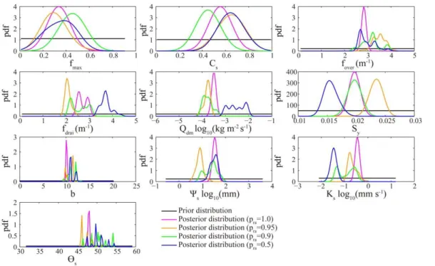
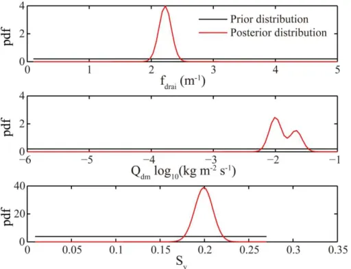
Using monthly heat flux data during 2003–2006 at the US-ARM site, we conducted

5

inversion of ten CLM parameters with four reference acceptance probabilities. Figure 1 shows the prior and posterior distributions of the parameters, where the prior distri-butions are derived from prior information, and the posterior distridistri-butions are derived

based on the last 200 samples of inverse modeling. Note that three parametersQdm,

Ψs, and Ks vary by several orders of magnitude, and are log10-transformed.

Poste-10

rior distributions with different reference acceptance probabilities generally are

consis-tent, except forfdrai,Qdm and Sy when the rejection rate is very low with a reference

acceptance probability pra of 0.5. As shown in Eq. (3), a low reference acceptance

probability p_ra means that the rejection standard and searching ranges are relaxed.

As more potential estimates are identified and accepted, the bounds of posterior

dis-15

tributions increase, and multi-modal behaviors occur, especially for θs. The posterior

means/modes of the estimated parameters shifted farther or less away from the prior

means, particularly forfover andθs.

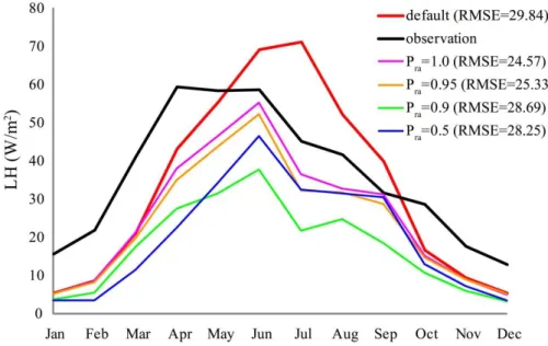
Figure 2 shows the simulated monthly mean heat fluxes using posterior estimates of parameters with four reference acceptance probabilities using monthly observations at

20

the US-ARM site. The black line shows the monthly mean heat fluxes obtained from ob-servations during 2003–2006, and the red line shows the calculated monthly mean heat fluxes using default parameters based on prior information. Simulations using default parameter values overestimate the heat fluxes in summer (from May to September), and underestimate in winter at the US-ARM site. When the reference probabilities are

25

(13)

HESSD

10, 5077–5119, 2013

Y. Sun et al.

Title Page

Tables Figures

◭ ◮

Back Close

Full Screen / Esc

Discussion

P

a

per

|

Dis

cussion

P

a

per

|

Discussion

P

a

per

|

Discussio

n

P

a

per

of Gaussian probabilities of misfits between calculated and observed responses) are 0.730, 0.730, and 0.728 respectively, which are greater than 0.636 for the default pa-rameter values. However the estimates with reference acceptance probability of 0.5 noticeably deviate from other inversion estimates, and tend to result in underestimates of simulated heat fluxes in summer. However, none of the parameter estimates is able

5

to yield much better fits during winter, which might be due to errors in the observed heat fluxes, errors in the CLM forcing data, and/or under-representation of the complicated physical processes using the current parameterization schemes.

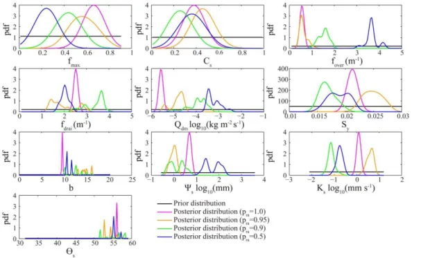
Similarly, inversion was also performed using monthly heat flux data during 2004–

2007 at the US-MOz site with different soil and vegetation cover from US-ARM site.

10

Figure 3 shows the posterior distributions of ten parameters with four reference

accep-tance probabilities. They show consistent patterns for different reference acceptance

probabilities, except for the parameterb. Even when the reference acceptance

proba-bility is 0.5, the inversion yields reasonable parameter estimates for most parameters

except forbandΨs. The relaxed rejection standard also leads to multi-modal, extended

15

posterior distribution bounds, and more potential parameter estimates. It is noted that

the posterior distribution off_max,C_s,f_drai,b, andΨs are around the median values of

the prior bounds.

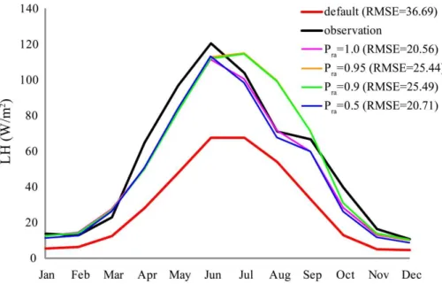
Figure 4 shows the calculated monthly mean heat fluxes using the posterior parame-ter estimates from monthly observation at the US-MOz site. It is obvious that the default

20

simulation underestimates the heat flux over all seasons. From January to June, all

posterior estimates with different reference acceptance probabilities can significantly

improve the simulation of heat flux, except for some small underestimations in April, May, and June. From July to December, the posterior estimates with reference accep-tance probabilities of 1.0 and 0.5 are similar and close to observation, while the other

25

(14)

HESSD

10, 5077–5119, 2013

Y. Sun et al.

Title Page

Tables Figures

◭ ◮

Back Close

Full Screen / Esc

Discussion

P

a

per

|

Dis

cussion

P

a

per

|

Discussion

P

a

per

|

Discussio

n

P

a

per

|

greater than 0.876 of the default simulation. Differences in the posterior distributions

with different reference acceptance probabilities are small.

4.1.2 Posterior distributions of input parameters and simulated heat flux from use of daily data

Figure 5 shows the posterior distribution of model parameters with four reference

ac-5

ceptance probabilities using daily heat flux data during 2003–2006 at the US-ARM site. The posterior distributions disperse over the prior bounds for most parameters. Among the four sets of posterior distributions, reference acceptance probability of 1.0 and 0.95

identify similar bounds, while the other two sets yield different results, particularly for

fmax,fover,Qdm, andKs. Moreover, multi-modal distributions occur for most parameters

10

when the rejection standard is relaxed.

Figure 6 shows the calculated monthly mean heat fluxes using the posterior esti-mates of parameters from daily observations at the US-ARM site. The posterior es-timates of parameters also improve the heat flux in summer. The acceptance proba-bilities of the simulations with four parameter sets are 0.636, 0.618, 0.584, and 0.593

15

respectively, which are all greater than 0.579 of the default simulation.

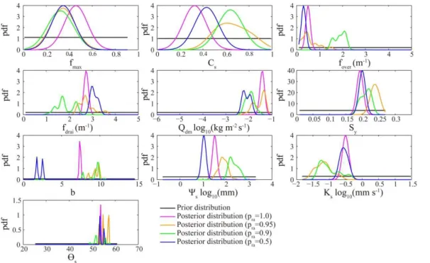
The posterior distributions of the parameters with the four reference acceptance probabilities using daily heat flux data during 2004–2007 at the US-MOz site show

that the posterior distributions are more consistent forCs,fover,Qdm,Sy, and Ψs, but

dispersed forb,Ksandθs. When the rejection standard is relaxed, the posterior bounds

20

can become much wider, especially forf_drai, Q_dm, b,K_s and θ_s. In winter, all

(15)

HESSD

10, 5077–5119, 2013

Y. Sun et al.

Title Page

Tables Figures

◭ ◮

Back Close

Full Screen / Esc

Discussion

P

a

per

|

Dis

cussion

P

a

per

|

Discussion

P

a

per

|

Discussio

n

P

a

per

4.2 Parameter inversion at MOPEX sites using runoffobservations

Runoffobservations are also used in the inverse modeling of CLM. Figure 7 shows the

posterior distribution of the parameters with four reference acceptance probabilities

using monthly runoff data during 2002–2005 at the MOPEX basin close to US-ARM.

Posterior distributions with strict reference acceptance probabilities (e.g. 1.0, 0.95 and

5

0.9) have consistent patterns for most parameters, except for b, K_s, and θ_s. It is

in-teresting to see thatfmax is identically estimated by inversions with different reference

acceptance probabilities. When the rejection standards are relaxed, the bounds of pos-terior distributions of most parameters become wider, and multi-modal patterns occur.

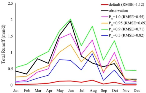
Figure 8 shows the calculated monthly mean runoff using the posterior estimates

10

of parameters from monthly observations at the MOPEX basin. The default simulation

barely shows any variability of runoff. The posterior estimates significantly improve the

runoffsimulations in all seasons, albeit larger variability than observations is noted from

July to October. The acceptance probabilities are 0.846, 0.767, 0.758, and 0.737, all

greater than 0.707 of the default runoffsimulation. Among the four sets of simulations

15

based on inversion, more stringent sample rejection criterion results in a better match between the simulated responses with observations.

For comparison with inversion using monthly runoffdata, we also perform inversion

using daily runoffdata during 2002-2005 at the MOPEX basin. The posterior

distribu-tions with different reference acceptance probabilities disperse over the prior bounds,

20

except forSy. The calculated monthly mean runoffvalues using the posterior estimates

of parameters from daily observation are reasonable. Posterior estimates with

refer-ence acceptance probabilities of 1.0 and 0.95 can significantly improve the runoff

sim-ulation over all seasons, but underestimate the runoffin summer, and overestimate the

runoffin winter.

(16)

HESSD

10, 5077–5119, 2013

Y. Sun et al.

Title Page

Tables Figures

◭ ◮

Back Close

Full Screen / Esc

Discussion

P

a

per

|

Dis

cussion

P

a

per

|

Discussion

P

a

per

|

Discussio

n

P

a

per

|

5 Results of subset parameter inversion

Our global sensitivity analyses across 13 flux towers and 20 MOPEX basins,

sug-gest that simulated LH and runoffare most sensitive to three subsurface parameters.

Because the other parameters are less identifiable, the inverse problem will be less ill-posed by fixing the trivial parameters. In this section, we test the feasibility of only

5

inverting a subset of identifiable parameters to determine if similar or improved model skill may be achieved compared to using the full-set parameter inversion results. We first conducted the inversion with a reduced set of parameters using monthly observa-tion at the two flux tower sites and the MOPEX basin.

Figure 9 shows the posterior distribution of the reduced set of parameters at the

US-10

MOz site. Compared with the results of ten parameters (see Figure 3), the medians of

the posterior distribution offdraiandQdmare smaller, the width of the posterior bounds

off_draiandS_yis unchanged, while that ofQ_dmexpands.

Figure 10 shows the calculated monthly mean heat flux using posterior estimates of parameters at the US-MOz site. The simulations using posterior estimates of the

15

reduced parameter set significantly improve the heat flux simulation over all seasons, and are similar to the results of inversion with ten parameters.

Inversion at the US-ARM site also show that in general, the posterior bounds start to narrow, and the multi-modal patterns disappear, compared to the inversion results with the full-set of parameters. Using posterior estimates of the reduced parameter set can

20

significantly improve the latent heat flux simulations compared to the results using the full-set of parameters, especially from October to December, and from January to May. Figure 11 shows the posterior distribution of the reduced parameters at the MOPEX basin. Compared with the results of ten parameters (see Fig. 7), the medians of

poste-rior distribution off_drai andQ_dm are smaller, while that ofS_y does not change, and the

25

widths of posterior distribution of all parameters stay the same.

Figure 12 shows the calculated monthly mean runoffusing posterior estimates of

(17)

HESSD

10, 5077–5119, 2013

Y. Sun et al.

Title Page

Tables Figures

◭ ◮

Back Close

Full Screen / Esc

Discussion

P

a

per

|

Dis

cussion

P

a

per

|

Discussion

P

a

per

|

Discussio

n

P

a

per

simulation, which is similar to the posterior simulation with ten parameters, while the simulation with the default parameter is far away from observation.

Overall, inverse modeling with a reduced set of parameters identified from previous sensitivity analysis shows some small improvements in simulating heat flux compared to using the posterior results with ten parameters, and since the inverse problems

be-5

come less ill-posed with fewer unknowns, the convergence of inverse modeling is faster and the resulting posteriors are more consistent without multi-modal patterns. However,

the simulations of heat flux at the US-MOz and runoffat the MOPEX basin are

com-parable between the inversion for the reduced and full set of parameters. Theoretically, one may expect improvement using the reduced parameter set because the inversion

10

become less ill-posed, but in practice, getting a faster convergence of the solution may be the main advantage, which is important especially when calibrating parameters for computationally intensive models.

6 Discussion

6.1 Impacts of temporal resolution of heat flux observation on inverse modeling

15

Both monthly and daily heat flux data have been used in the inverse modeling at se-lected flux tower sites. Using monthly observation data, inversion with reference

accep-tance probabilities (except forpraof 0.5 at US-ARM) is able to identify proper parameter

estimates to improve heat flux simulation. Using daily observation data, inversion im-proves the heat flux simulation only with reference acceptance probabilities of 1.0 and

20

0.95, suggesting that increasing data frequency requires a more stringent acceptance criterion. Comparing Figures 1 and 5, inversion using daily instead of monthly

obser-vations favors values offover,Qdm,Ψs towards the lower bounds butθs is opposite at

the US-ARM site. At the US-MOz site, inversion using daily observation also favors

values off_over,Q_dmtowards the lower bounds butK_sis opposite. Hence, finer temporal

(18)

HESSD

10, 5077–5119, 2013

Y. Sun et al.

Title Page

Tables Figures

◭ ◮

Back Close

Full Screen / Esc

Discussion

P

a

per

|

Dis

cussion

P

a

per

|

Discussion

P

a

per

|

Discussio

n

P

a

per

|

resolution of observation data all favors smallerfover andQdm. For specific site, it may

also lead to changes of other parameters.

Regarding inversion using runoff data, we also found that finer temporal resolution

of runoff observations leads to more dispersion of the posterior distributions of most

parameters, except for f_over, S_y and θ_s. Using monthly observation data, inversions

5

with all reference acceptance probabilities are able to improve monthly mean runoff

simulation over all seasons. However using daily observation data, inversion improves

runoffsimulation only with reference acceptance probabilities of 1.0 and 0.95.

Overall, finer temporal resolution of observation data leads to more dispersion of the posterior distributions and increases the risk of using relaxed rejection standard. These

10

are likely related to increased measurement errors, data redundancy, and over-fitting with higher temporal frequency observations.

6.2 Impacts of soil and vegetation cover on inverse modeling

Compared to US-MOz, inverse modeling at the US-ARM site identifies smallerQdm,

and greaterf_over,θ_s. In addition, the bounds of posterior distribution identified by the

15

inversion show more consistency across different reference acceptance probabilities

forfover,fdrai,Qdm,b, andΨsat US-ARM than US-MOz, especially with monthly heat

flux data. At US-MOz, the bounds of posterior distribution are mainly consistent forf_max,

fover,Qdm,Sy, andθs. These inversion results are consistent with the sensitivity analysis

performed by Hou et al. (2012), which shows larger sensitivity to the respective

param-20

eters at the two sites related to the soil and vegetation properties. The best estimated

parameters are different at sites with different climate, land use, and soil conditions;

hence soil and vegetation cover may inform the selection of sensitive parameters that can be used in reduced parameter sets for inverse modeling. It is therefore neces-sary to analyze parameter sensitivity and identifiability across the MOPEX basins and

25

classify them into different groups/classes with similar climate and soil conditions, and

(19)

HESSD

10, 5077–5119, 2013

Y. Sun et al.

Title Page

Tables Figures

◭ ◮

Back Close

Full Screen / Esc

Discussion

P

a

per

|

Dis

cussion

P

a

per

|

Discussion

P

a

per

|

Discussio

n

P

a

per

6.3 Impacts of reference acceptance probability

In this study, we set the reference acceptance probability in the inverse modeling to relax rejection standard to allow more freedom in searching for optimal parameter es-timates. However, relaxing the rejection standard leads to broadening of the bounds of posterior distribution and multi-modal behaviors. That is, the posterior estimates tend to

5

be more “accurate” but less “precise”, and the corresponding inversion process usually take longer to converge.

6.4 Impacts of different types of observations on inverse modeling

Inverse modeling using heat flux at US-ARM and runoff at the MOPEX basin, which

is located close to US-ARM, provides an opportunity to assess the impacts of data

10

type on inverse modeling. Comparing Fig. 1 and Fig. 7, the posterior distributions that

optimize the simulations of heat flux can differ from those that optimize the simulations

of runoff. Since the calibrated model parameters are directly related to soil hydrological

processes including surface and subsurface runoff, it is not surprising that model

in-version leads to more significant improvements in runoff(Fig. 8) than heat flux (Fig. 2)

15

compared to simulations that use the default parameter values. The simulations of heat flux can nevertheless be improved by inverting hydrologic parameters because surface

heat flux is influenced by soil moisture, which is closely related to runoffprocesses. The

improvement in simulations of heat flux is particularly noticeable for US-MOz, where the surface energy budget is more strongly influenced by soil moisture in a forested

20

site compared to US-ARM, which is a cropland site.

Although inversion modeling leads to larger improvements in the runoffsimulations

compared to the simulations using the default parameter values, the runoffsimulations

with the posterior estimates still deviate quite significantly from the observed runoffin

late summer and fall. This suggests that some model biases in runoffmay require

struc-25

(20)

HESSD

10, 5077–5119, 2013

Y. Sun et al.

Title Page

Tables Figures

◭ ◮

Back Close

Full Screen / Esc

Discussion

P

a

per

|

Dis

cussion

P

a

per

|

Discussion

P

a

per

|

Discussio

n

P

a

per

|

6.5 Improvements through Bayesian model averaging

For each reference acceptance probability for the MCMC-Bayesian inversion, one can obtain a set of posterior distributions of the unknowns. Bayesian model averaging is

used to integrate the different sets of predictions by weighting the posteriors according

to their posterior model probability.

5

By integrating inversion results of different reference acceptance probabilities,

Bayesian model averaging produces smoother posterior distributions. Figure 13 shows the posterior distributions of the parameters through Bayesian model averaging at the US-ARM site. The black lines represent the prior distributions based on prior informa-tion. The red and blue curves represent the posterior distributions of the parameters

10

using monthly and daily heat flux observations, respectively. These two sets of

poste-rior distributions are similar to each other for most parameters, except for fover. Daily

heat flux favors smallerC_s,f_over,Q_dm,Ψs, and greaterfmax,Ks,θs. The posterior

distri-butions using monthly and daily observations at the US-MOz site are also similar, but daily heat flux favors smallerCs,fover,fdrai,Qdm,Sy,Ψs,θs, and greaterfmax,Ks.

15

Figure 14 shows the posterior distribution of the parameters through Bayesian model averaging at the MOPEX basin. The posterior distributions using monthly and daily

runoffobservation are also similar. Daily observation favors smallerθs and greaterSy,

b,K_s. It is noted that the differences between the posterior distributions from monthly

and daily data are even smaller from inversion using runoffcompared to inversion using

20

heat flux, especially forfdrai,Qdm. This may be related to the characteristic time scales

of the physical processes. Surface heat flux may have less day-to-day variability (hence

larger data redundancy) compared to runoff, which responds more directly to

precipita-tion that has larger temporal variability during the wet season. These differences could

be site and season dependent so analyses over a larger number of sites can provide

25

(21)

HESSD

10, 5077–5119, 2013

Y. Sun et al.

Title Page

Tables Figures

◭ ◮

Back Close

Full Screen / Esc

Discussion

P

a

per

|

Dis

cussion

P

a

per

|

Discussion

P

a

per

|

Discussio

n

P

a

per

Model integration represents a compromise of all possibilities of the inversion setup. In general, it results in “safer” (i.e. more likely to be unbiased) estimates but lower resolution (i.e. wider posterior distributions).

6.6 Model validation

In the above analyses, we compared observed and model calibrated responses to

5

check whether smaller misfits can be achieved through the calibration process, and

to evaluate the different calibration power using runoff versus heat flux observations,

monthly versus daily data, and different tuning parameters. In an inverse study, it is

important to validate the inversion approach. It is straightforward to validate the results when true values of the unknown input parameters are available. Otherwise, people

10

may design “synthetic” models by assuming the “true” parameter values are available, then “generate” the corresponding “true” responses, which are then used for testing the inversion approach. An alternative way of validation is to separate the dataset to training (for calibrating the parameters) and testing periods, assuming the parameters are intrinsic to the system and not time-varying. Figure 15a and b show the

obser-15

vations as well as model simulated monthly and daily runoff calculated using default

and optimal parameter values. The inversion (training) time period is 2002–2005, and validation periods are 2000–2001 and 2006–2008. The root-mean-square-errors (RM-SEs) are calculated for the validation periods only. We found that RMSEs are reduced

more for monthly data than for daily data. In general, runoffcalculations using optimal

20

(22)

HESSD

10, 5077–5119, 2013

Y. Sun et al.

Title Page

Tables Figures

◭ ◮

Back Close

Full Screen / Esc

Discussion

P

a

per

|

Dis

cussion

P

a

per

|

Discussion

P

a

per

|

Discussio

n

P

a

per

|

7 Conclusions

In this study, we demonstrated the possibility of inverting hydrologic parameters using

surface flux and runoffobservations in CLM4. Calibrating model parameters using the

deterministic least–square fitting method provides little improvement in simulating heat

flux and runoff, but using the calibrated values as initial guesses in the MCMC-Bayesian

5

calibration reduces the discrepancies between simulated and observed responses, but

the convergence rate is unaffected by the choice of initial guesses.

Focusing on the MCMC-Bayesian inversion method, we conducted inverse model-ing at two flux tower sites and one MOPEX basin. We also discussed the impacts of relaxing the rejection standard, data temporal resolution, data types, and soil and

10

vegetation on parameter inference. Informed by our previous sensitivity analysis, we also performed inversion with reduced parameter dimensionality. Moreover, Bayesian

model averaging is adopted to integrate the posterior estimates with different reference

acceptance probabilities. The major conclusions are as follows.

1. Inversion results at the flux tower and MOPEX sites using monthly and daily

sur-15

face flux and runoff observations show that the MCMC-Bayesian inversion

ap-proach effectively and reliably improves the simulation of CLM under different

cli-mates and environmental conditions.

2. Temporal resolution of observations has clear impacts on the results of inverse

modeling using heat flux data, but the impacts are smaller using runoffdata. Due

20

to data redundancy and quality, finer temporal resolution of observations may yield biased estimates and multi-modal posterior distributions.

3. Significant improvements can be achieved to better match the simulated and

ob-served heat flux and runoffby using the estimated parameters compared to

us-ing the default parameter values. The improvement is more significant for runoff

25

than heat flux because the calibrated parameters are more directly related to

(23)

HESSD

10, 5077–5119, 2013

Y. Sun et al.

Title Page

Tables Figures

◭ ◮

Back Close

Full Screen / Esc

Discussion

P

a

per

|

Dis

cussion

P

a

per

|

Discussion

P

a

per

|

Discussio

n

P

a

per

especially in areas (e.g. forest) where the constraints between energy and water are stronger. Soil and vegetation cover have important impacts on parameter

sen-sitivities, leading to the different patterns of posterior distributions of parameters

at different sites.

4. Reducing the parameter set can make the inverse problem less ill-posed.

Numer-5

ically, it also speeds up the convergence. In this study, inverse modeling with the reduced parameter set favors parameter estimates closer to the lower bounds than using the full set of parameters.

5. Bayesian model averaging that integrates the posterior estimates with different

reference acceptance probabilities, can smooth the posterior distribution and

pro-10

vide more reliable parameter estimates, but at the expense of wider uncertainty bounds.

Overall, the MCMC-Bayesian inversion approach is found to provide effective and

re-liable estimates of model parameters at the site and watershed level to improve CLM

simulations of surface flux and runoff. To apply the method for inversion over a region

15

or globally, there are a number of challenges, including computational requirements and availability and quality of observation data. The analyses presented in this study should be extended to a larger number of sites with a wider range of climate, hydro-logic, and vegetation/soil conditions to determine if and how model parameters may be transferrable based on site conditions to larger areas or river basins. Exploring model

20

inversion at the river basin level rather than site level using combinations of local flux measurements, area averaged flux data (e.g. derived from satellite), and basin total

runoff, each with their own uncertainty estimates, may provide an alternative strategy

for calibrating model parameter values for each river basin. To reduce the computa-tional demand, we will also test the performance of the MCMC-Bayesian inversion

25

(24)

HESSD

10, 5077–5119, 2013

Y. Sun et al.

Title Page

Tables Figures

◭ ◮

Back Close

Full Screen / Esc

Discussion

P

a

per

|

Dis

cussion

P

a

per

|

Discussion

P

a

per

|

Discussio

n

P

a

per

|

Acknowledgements. This work is supported by the project “Climate Science for a Sustainable Energy Future” funded by the DOE Earth System Modeling Program. The Pacific Northwest National Laboratory (PNNL) Platform for Regional Integrated Modeling and Analysis (PRIMA) Initiative provided support for the model configuration and datasets used in the numerical ex-periments. PNNL is operated for the US DOE by Battelle Memorial Institute under Contract

5

DE-AC06-76RLO1830. Yu Sun and Fuqiang Tian would like to acknowledge the support from the National Science Foundation of China (NSFC51190092, 51222901) and the foundation of the State Key Laboratory of Hydroscience and Engineering of Tsinghua University (2012-KY-03).

References

10

Allison, V. J., Miller, R. M., Jastrow, J. D., Matamala, R., and Zak, D. R.: Changes in Soil Micro-bial Community Structure in a Tallgrass Prairie Chronosequence, Soil Sci. Soc. Am. J., 69, 1412–1421, doi:10.2136/sssaj2004.0252, 2005.

Baer, S. G., Kitchen, D. J., Blair, J. M., and Rice, C. W.: Changes in ecosystem structure and function along a chronosequence of restored grasslands, Ecol. Appl., 12, 1688–1701,

15

10.1890/1051-0761(2002)012[1688:ciesaf]2.0.co;2, 2002.

Beven, K. and Binley, A.: The future of distributed models: Model calibration and uncertainty prediction, Hydrol. Process., 6, 279–298, doi:10.1002/hyp.3360060305, 1992.

Boyle, D. P., Gupta, H. V., and Sorooshian, S.: Toward improved calibration of hydrologic mod-els: Combining the strengths of manual and automatic methods, Water Resour. Res., 36,

20

3663–3674, doi:10.1029/2000wr900207, 2000.

Chen, J., Hoversten, G. M., Vasco, D., Rubin, Y., and Hou, Z.: Joint inversion of seismic AVO and EM data for gas saturation estimation using a sampling-based stochastic model, 2004 SEG Annual Meeting, 2004,

Cosby, B. J., Hornberger, G. M., Clapp, R. B., and Ginn, T. R.: A Statistical Exploration of

25

the Relationships of Soil Moisture Characteristics to the Physical Properties of Soils, Water Resour. Res., 20, 682–690, doi:10.1029/WR020i006p00682, 1984.

Cosgrove, B. A., Lohmann, D., Mitchell, K. E., Houser, P. R., Wood, E. F., Schaake, J. C., Robock, A., Marshall, C., Sheffield, J., Duan, Q., Luo, L., Higgins, R. W., Pinker, R. T., Tarpley, J. D., and Meng, J.: Real-time and retrospective forcing in the North

(25)

HESSD

10, 5077–5119, 2013

Y. Sun et al.

Title Page

Tables Figures

◭ ◮

Back Close

Full Screen / Esc

Discussion

P

a

per

|

Dis

cussion

P

a

per

|

Discussion

P

a

per

|

Discussio

n

P

a

per

American Land Data Assimilation System (NLDAS) project, J. Geophys. Res., 108, 8842, doi:10.1029/2002jd003118, 2003.

Doherty, J.: PEST, Model Independent Parameter Estimation, 2008.

Duan, Q., Sorooshian, S., and Gupta, V.: Effective and efficient global optimization for con-ceptual rainfall-runoffmodels, Water Resour. Res., 28, 1015–1031, doi:10.1029/91wr02985,

5

1992.

Duan, Q. Y., Gupta, V. K., and Sorooshian, S.: Shuffled Complex Evolution Approach for Eff ec-tive and Efficient Global Minimization, J. Optimiz. Theory App., 76, 501–521, 1993.

Feyen, L., Vrugt, J. A., Nuall ´ain, B. ´O., van der Knijff, J., and De Roo, A.: Parameter optimisa-tion and uncertainty assessment for large-scale streamflow simulaoptimisa-tion with the LISFLOOD

10

model, J. Hydrol., 332, 276–289, doi:10.1016/j.jhydrol.2006.07.004, 2007.

Fischer, M. L., Billesbach, D. P., Berry, J. A., Riley, W. J., and Torn, M. S.: Spatiotemporal variations in growing season exchanges of CO₂, H₂O, and sensible heat in agricultural fields of the Southern Great Plains, Earth Interact., 11, 1–21, doi:10.1175/EI231.1, 2007.

Freer, J., Beven, K., and Ambroise, B.: Bayesian Estimation of Uncertainty in RunoffPrediction

15

and the Value of Data: An Application of the GLUE Approach, Water Resour. Res., 32, 2161– 2173, doi:10.1029/95wr03723, 1996.

Gu, L., Meyers, T., Pallardy, S. G., Hanson, P. J., Yang, B., Heuer, M., Hosman, K. P., Riggs, J. S., Sluss, D., and Wullschleger, S. D.: Direct and indirect effects of atmospheric condi-tions and soil moisture on surface energy partitioning revealed by a prolonged drought at a

20

temperate forest site, J. Geophys. Res., 111, D16102, doi:10.1029/2006jd007161, 2006. Gu, L., Massman, W. J., Leuning, R., Pallardy, S. G., Meyers, T., Hanson, P. J., Riggs, J. S.,

Hos-man, K. P., and Yang, B.: The fundamental equation of eddy covariance and its application in flux measurements, Agr. Forest Meteorol., 152, 135–148, 2012.

Gupta, H. V., Sorooshian, S., and Yapo, P. O.: Toward improved calibration of hydrologic models:

25

Multiple and noncommensurable measures of information, Water Resour. Res., 34, 751–763, doi:10.1029/97wr03495, 1998.

Hadamard, J.: Sur les probl èmes aux d ériv ées partielles et leur signification physique, Prince-ton University Bulletin, 49–52, 1902.

Hou, Z. and Rubin, Y.: On minimum relative entropy concepts and prior compatibility

is-30

(26)

HESSD

10, 5077–5119, 2013

Y. Sun et al.

Title Page

Tables Figures

◭ ◮

Back Close

Full Screen / Esc

Discussion

P

a

per

|

Dis

cussion

P

a

per

|

Discussion

P

a

per

|

Discussio

n

P

a

per

|

Hou, Z., Rubin, Y., Hoversten, G. M., Vasco, D., and Chen, J. S.: Reservoir-parameter identifi-cation using minimum relative entropy-based Bayesian inversion of seismic AVA and marine CSEM data, Geophysics, 71, O77–O88, doi:10.1190/1.2348770, 2006.

Hou, Z., Huang, M., Leung, L. R., Lin, G., and Ricciuto, D. M.: Sensitivity of surface flux sim-ulations to hydrologic parameters based on an uncertainty quantification framework applied

5

to the Community Land Model, J. Geophys. Res., 117, D15108, doi:10.1029/2012jd017521, 2012.

Hoversten, G. M., Cassassuce, F., Gasperikova, E., Newman, G. A., Chen, J., Rubin, Y., Hou, Z., and Vasco, D.: Direct reservoir parameter estimation using joint inversion of marine seis-mic AVA and CSEM data, Geophysics, 71, C1–C13, 2006.

10

Huang, M., Hou, Z., Leung, L. R., Ke, Y., Liu, Y., Fang, Z., and Sun, Y.: Uncertainty Analysis of RunoffSimulations and Parameter Detectability in the Community Land Model – Evidence from MOPEX Basins and Flux Tower Sites, J. Hydrometeorol., accepted, 2013.

Ke, Y., Leung, L. R., Huang, M., Coleman, A. M., Li, H., and Wigmosta, M. S.: Development of high resolution land surface parameters for the Community Land Model, Geosci. Model Dev.,

15

5, 1341–1362, doi:10.5194/gmd-5-1341-2012, 2012.

Klepper, O., Scholten, H., and Van Kamer, J. P. G. D.: Prediction uncertainty in an ecological model of the oosterschelde estuary, Journal of Forecasting, 10, 191–209, doi:10.1002/for.3980100111, 1991.

Kollat, J. B., Reed, P. M., and Wagener, T.: When are multiobjective calibration trade-offs in

hy-20

drologic models meaningful?, Water Resour. Res., 48, W03520, doi:10.1029/2011wr011534, 2012.

Kuczera, G. and Parent, E.: Monte Carlo assessment of parameter uncertainty in conceptual catchment models: the Metropolis algorithm, J. Hydrol., 211, 69–85, 1998.

Riley, W. J., Biraud, S. C., Torn, M. S., Fischer, M. L., Billesbach, D. P., and Berry, J. A.: Regional

25

CO₂and latent heat surface fluxes in the Southern Great Plains: Measurements, modeling, and scaling, J. Geophys. Res.-Biogeo., 114, G04009, doi:10.1029/2009jg001003, 2009. Sorooshian, S.: Parameter-Estimation of Rainfall – Runoff Models with Heteroscedastic

Streamflow Errors – the Non-Informative Data Case, J. Hydrol., 52, 127–138, 1981.

Sorooshian, S. and Dracup, J. A.: Stochastic Parameter-Estimation Procedures for Hydrologic

30

(27)

HESSD

10, 5077–5119, 2013

Y. Sun et al.

Title Page

Tables Figures

◭ ◮

Back Close

Full Screen / Esc

Discussion

P

a

per

|

Dis

cussion

P

a

per

|

Discussion

P

a

per

|

Discussio

n

P

a

per

Sorooshian, S., Duan, Q. Y., and Gupta, V. K.: Calibration of Rainfall-Runoff Models – Ap-plication of Global Optimization to the Sacramento Soil-Moisture Accounting Model, Water Resour. Res., 29, 1185–1194, 1993.

Suyker, A. E. and Verma, S. B.: Evapotranspiration of irrigated and rainfed maize-soybean cropping systems, Agr. Forest Meteorol., 149, 443–452, 2009.

5

Tarantola, A.: Inverse Problem Theory and Methods for Model Parameter Estimation, Society for Industrial and Applied Mathematics, Philadelphia, PA, USA, 2005.

Van Straten, G. T. and Keesman, K. J.: Uncertainty propagation and speculation in projective forecasts of environmental change: A lake-eutrophication example, J. Forecast., 10, 163– 190, doi:10.1002/for.3980100110, 1991.

10

Vrugt, J. A. and Robinson, B. A.: Improved evolutionary optimization from genetically adaptive multimethod search, P. Natl. Acad. Sci. USA, 104, 708–711, doi:10.1073/pnas.0610471104, 2007.

Vrugt, J. A., Gupta, H. V., Bastidas, L. A., Bouten, W., and Sorooshian, S.: Effective and efficient algorithm for multiobjective optimization of hydrologic models, Water Resour. Res., 39, 1214,

15

doi:10.1029/2002wr001746, 2003a.

Vrugt, J. A., Gupta, H. V., Bouten, W., and Sorooshian, S.: A Shuffled Complex Evolution Metropolis algorithm for optimization and uncertainty assessment of hydrologic model pa-rameters, Water Resour. Res., 39, 1201, doi:10.1029/2002wr001642, 2003b.

Vrugt, J. A., Diks, C. G. H., Gupta, H. V., Bouten, W., and Verstraten, J. M.: Improved treatment

20

of uncertainty in hydrologic modeling: Combining the strengths of global optimization and data assimilation, Water Resour. Res., 41, W01017, doi:10.1029/2004wr003059, 2005. Xia, Y., Mitchell, K., Ek, M., Cosgrove, B., Sheffield, J., Luo, L., Alonge, C., Wei, H., Meng,

J., Livneh, B., Duan, Q., and Lohmann, D.: Continental-scale water and energy flux anal-ysis and validation for North American Land Data Assimilation System project phase 2

25

(NLDAS-2): 2. Validation of model-simulated streamflow, J. Geophys. Res., 117, D03110, doi:10.1029/2011jd016051, 2012.

Yapo, P. O., Gupta, H. V., and Sorooshian, S.: Automatic calibration of conceptual rainfall-runoff