Samuel da Silva
Member, ABCM[email protected] State University of the West of Paraná- UNIOESTE Centro de Engenharias e Ciências Exatas Foz do Iguaçu, PR, Brazil.
Scott Cogan
[email protected]Emmanuel Foltête
[email protected]Université de Franche-Comté Institut FEMTO-ST, Département LMARC Besançon, France
Fabrice Buffe
[email protected] Centre National d’Etudes Spatiales –CNES Centre Spatial de Toulouse 31401 Toulouse, FranceMetrics for Nonlinear Model Updating
in Structural Dynamics
The aim of this paper is to perform a comparative study between different distance measures or metrics for use in nonlinear model updating using vibration test data. Four metrics derived from both frequency and time domain updating approaches are studied, including the harmonic balance method, the constitutive equation error, the restoring force surface and the Karhunen-Loève decomposition. In the first section, a benchmark model with local nonlinear stiffness is defined in order to illustrate each method. Secondly, each nonlinear updating metric is succinctly reviewed. Finally, the relative performances of the different metrics are investigated based on numerical simulations. These results allow us to characterize the applicability and limitations of the different approaches.
Keywords: nonlinear model updating, harmonic balance, constitutive relation error, restoring force surface, Karhunen-Loève decomposition
Introduction
1
Local methods for linear model updating based on vibration data are well-documented in the literature (Friswell and Mottershead, 1995). In general, the goal is to solve an inverse problem involving objective functions that represent correlations between the experimental and numerical data from a model in which some parameters are unknown. Currently, these functions are computed using either modal quantities, e.g. natural frequencies, modal shapes or frequency response functions (FRF). Unfortunately, if the structure presents any nonlinearity, these procedures often fail. Fundamentally speaking, the principal reason for this failure is that linear modal parameters are functions of relationships based on a unidimensional convolution while nonlinear systems follow multidimensional convolutions.
Nonlinear effects are becoming important in lightweight and flexible modern engineering structures due to the presence of joints, backlash, friction, stiffening nonlinearities, large displacement amplitudes, etc. Thus, if these nonlinear effects are not taken into account, then the linear model updating procedure will not necessarily converge properly, and the resulting model predictions will be erroneous (Kerschen et al., 2006).
The domain of nonlinear structural dynamics is not as mature as its linear counterpart, and this is especially true for model updating methodologies. However, numerous recent works are dedicated to the identification of the local nonlinear parameters of a model based on a variety of frequency and/or time domain methods.
A classical approach is to consider the multidimensional high-order FRFs as linearized FRFs using the first high-order harmonic balanced (HB) method to obtain a suitable model description in the frequency domain. Meyer and Link (2003) employed the HB method to update nonlinear two-degree-of-freedom elements in a
Paper accepted November, 2008. Technical Editor: Domingos A. Rade.
larger linear finite element model (FEM). Böswald and Link (2004) applied the HB method in a similar way to update nonlinear joint parameters. The main advantage of this method is that it allows us to perform nonlinear updating using FRF residuals. However, the HB method fails when working with complex nonlinearities due to the loss of information caused by the linearization procedure.
Another linear updating approach in the frequency domain that can be adapted for nonlinear updating is the method based on the constitutive relation error (CRE). The CRE is based on a separation between the reliable equations, e.g. the equilibrium equations, and the less reliable equations, e.g. the constitutive relations (Deraemaeker et al., 2002). Puel (2001) investigated an extension of CRE for nonlinear model updating employing the HB method to obtain linear FRFs. In this case, the same weaknesses shown by the HB method were observed. The author concludes that the frequency domain methods are not well-adapted for nonlinear identification.
A more effective frequency domain technique is to consider the concept of high-order FRFs using Volterra series. However the results produced have been limited by the fact that a low-order truncation of the series is in general required (Worden and Manson, 2005). Campello et al. (2004) proposed Laguerre filters to describe a discrete-time Volterra series in order to overcome this limitation and to be able to work with high-order kernels in the model.
Time domain procedures may be more promising than frequency domain methodologies because it is possible to avoid the transformation between domains, a difficult procedure in nonlinear system analysis. Various authors have already investigated this possibility. Schmidt (1994) proposed a methodology to update local nonlinearities, such as Coulomb friction, gaps and local plasticity in a FE model employing conventional modal state observers for the linearized model.
mass matrix be known in advance, this approach is difficult to implement in complex structures.
A more efficient time domain methodology is based on the proper orthogonal decomposition (POD) of the covariance matrix constructed from response time histories. The POD is also known as the Karhunen-Loève decomposition or principal component analysis (PCA). These concepts are mainly used in structural dynamics for compressing vector data (Silva et al., 2007). Lenaerts et al. (2001) used the POD of the displacement vector to identify the nonlinear parameters combined with an optimization procedure based on the differences between the experimental and simulated POD. Zhang and Guo (2007) combined the POD with a design of experiments (DOE) in order to update nonlinear material parameters based on strain measurements with uncertainty considerations. The DOE followed the work of Schultze et al. (2001). These examples and numerous others in the literature show that the POD is a suitable and promising indicator for nonlinear model updating. However, the decomposition is essentially a linear tool, and there are some difficulties that must be overcome in the future.
The reader interested in a detailed review of frequency and time domain techniques for nonlinear model updating can consult the work of Kerschen et al. (2006).
The aim of the present paper is to examine, through numerical simulations, some practical aspects and limitations of some frequency and time domain methods for nonlinear model updating. The following approaches are compared: HB method, CRE, RFS and POD. Initially, a benchmark example is defined and used to simulate different levels of local nonlinearities (weak, medium and strong). The residuals adapted for nonlinear behaviors obtained by the various methods are succinctly described. The results are then interpreted and suggestions for improving each method are discussed.
Nomenclature
M mass matrix K stiffness matrix
md
K modified stiffness matrix C proportional damping matrix
nl
f vector of nonlinear force function x&
& acceleration vector x& velocity vector x displacement vector
xˆ displacement amplitude in steady state
( )
0x initial condition vector of displacement
( )
tF excitation force in the time domain
( )
ΩF excitation force in the frequency domain F excitation force amplitude [N]
m lumped mass [kg]
i
k linear spring [N/m]
i
c linear viscous damping [N.s/m]
nl
k nonlinear stiffness parameter [N/m3]
eq
H equivalent FRF
ex
H experimental FRF
( )
knlJ objective function
(
U,V,W)
eω constitutive relation error
( )
nl CRE kE CRE energy index p nonlinear updating parameter
[ ]
kz time response matrix
Benchmark Structure Description
The equations of motion for a nonlinear vibrating system can be written by:
( )
t Cx( )
t Kx( )
t fnl( ) ( )
x,x Ft xM&& + & + + & = (1)
where the vector fnl
( )
x,x& is a nonlinear function of displacementsx and velocities x&. In this paper the techniques are illustrated
using a two DOF example in which the first mass is connected to the
ground through a spring with a cubic stiffness knl =15 N/m3, (see
Fig. 1). In this case the equations of motion are given by:
(
)
(
)
( )
(
2 3)
2(
2 3)
2 2 1 2 1 02
3 1 2 2 2 2 1 2 1 1 2 1 1
= − − + + + +
= + − − + + + +
x k x c x k k x c c x m
t f x k x k x c x k k x c c x
m nl
& &
& &
& &
& &
Figure 1. Nonlinear model of the 2 DOF system.
The nonlinear system also has linear springs k1=1N/m,
15
2=
k N/m and k3=1N/m, linear viscous damping with
1 0
3 2
1 c c .
c = = = Ns/m and mass m=1kg. To obtain the frequency
responses one generated 4096 samples with a sampling rate of 100 Hz. The time responses for the time domain procedures were
obtained assuming the excitation force f
( )
t null, and usingdifferent initial displacement vectors. The vectors used are
( )
[
]
T. .5 0918 0
0 =
x for weak nonlinearities, x
( )
0 =[
1.0 0.918]
Tfor medium nonlinearities and x
( )
0 =[
2.2 0.918]
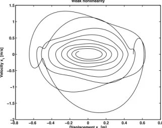
T for strongnonlinearities. Due to the assumed natures of the nonlinearity, it becomes clear that the larger the magnitudes of the initial displacements, the most important the nonlinear effects will be. The
phase plots for these conditions considering x1
( )
t and x&1( )
t areshown in Figs. 2 to 4. One can clearly see that the trajectories change as the initial condition vector varies.
−0.8 −0.6 −0.4 −0.2 0 0.2 0.4 0.6 0.8
−2 −1.5 −1 −0.5 0 0.5 1 1.5
Weak nonlinearity
Displacement x
1 [m]
Velocity x
1
[m/s]
For the frequency response analysis, sinusoidal excitations are applied in the frequency band from 0 to 2.5 Hz, using four increasing
amplitudes, namely F =0.1, 25F=0. , 5F=0. and 1 N. This
variation leads to increasing levels of nonlinear behavior. A classical downsampling procedure was performed to obtain a new sampling rate of 5 Hz, in order to improve the resolution near the equivalent linear modes. The frequency information of the two equivalent linear modes is in this range.
−1 −0.8 −0.6 −0.4 −0.2 0 0.2 0.4 0.6 0.8 1
−2.5 −2 −1.5 −1 −0.5 0 0.5 1 1.5 2 2.5
Medium nonlinearity
Displacement x
1 [m]
Velocity x
1
[m/s]
Figure 3. Phase portraits computed for medium nonlinearities.
−2 −1.5 −1 −0.5 0 0.5 1 1.5 2 2.5
−15 −10 −5 0 5 10 15
Strong nonlinearity
Displacement x
1 [m]
Velocity x
1
[m/s]
Figure 4. Phase portraits computed for strong nonlinearities.
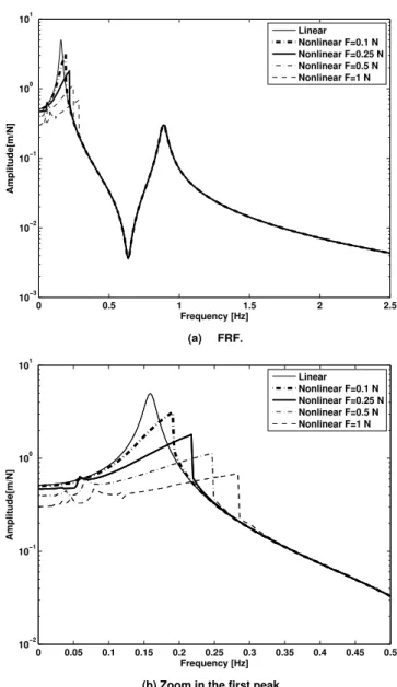
The plots of the ratio between the amplitudes of x1
( )
t and f( )
tare shown in Fig. 5. As can be seen, the resonance peaks change when the force amplitude is increased, (see Fig. 5b). This is a qualitative index of the presence of nonlinearity that affects mainly the first mode of the equivalent linear model. Several techniques can be used to detect nonlinear behaviors in experimental data, including the coherence functions, the Hilbert transform or the wavelet transform. These methodologies provide qualitative indicators for the presence of nonlinearities. The distortions between
the FRF curves indicate the nonlinear effects. Further details about these approaches can be found in (Worden and Tomlinson, 2001).
Metrics for Nonlinear Behavior
In this section, the metrics for nonlinear model updating obtained by several methods are reviewed. For the example considered herein, we assume for all the approaches that the nature and location of the nonlinearity are known.
0 0.5 1 1.5 2 2.5
10−3 10−2 10−1 100 101
Frequency [Hz]
Amplitude[m/N]
Linear Nonlinear F=0.1 N Nonlinear F=0.25 N Nonlinear F=0.5 N Nonlinear F=1 N
(a) FRF.
0 0.05 0.1 0.15 0.2 0.25 0.3 0.35 0.4 0.45 0.5
10−2 10−1 100 101
Frequency [Hz]
Amplitude[m/N]
Linear Nonlinear F=0.1 N Nonlinear F=0.25 N Nonlinear F=0.5 N Nonlinear F=1 N
(b) Zoom in the first peak.
Figure 5. Nonlinear FRF considering several levels of amplitude excitation.
Harmonic Balance Method
The harmonic balance method (HB) is a procedure to linearize the FRFs. The transformation to the frequency domain is performed by calculating the equivalent linear stiffness and damping parameters for the nonlinear elements (Böswald and Link, 2004). The fundamental assumption of the HB method is that the response of a nonlinear structure due to harmonic excitation can be approximated by a harmonic function of the frequency of excitation,
( )
(
)
( )
( )
( )
⎪ ⎩ ⎪ ⎨ ⎧ Ω Ω − ≈ Ω Ω ≈ Ω ≈ ⇒ + Ω = t sin xˆ x t cos xˆ x t sin xˆ x t sin fˆ t f 2 & & &ϕ (2)
In order to illustrate this approach, let us consider the simple case of a single degree of freedom system:
( ) ( )
x,x f t fx
m&&+ nl & = (3)
The nonlinear function fnl
( )
x,x& can be decomposed into aFourier series which can be truncated keeping only the fundamental terms:
( )
x,x& =a +a sin( )
Ωt +b cos( )
Ωt +Lfnl 0 1 1 (4)
where the coefficients a0,a1 and b1 are given by:
( )
ωπ π
∫
= 2 0 0 , 2 1 d x x f a nl &( ) ( )
ω ωπ π
∫
= 2 0 1 , 1 d cos x x f a nl &( ) ( )
ω ωπ π
∫
= 2 0 1 , 1 d sin x x f b nl &where ω=Ωt. The goal is to replace the nonlinear function
( )
x,xfnl & with equivalent elements. In the linear case:
( )
x,x k x c x k[
xˆsin( )
t]
c[
xˆcos( )
t]
fnl & = eq + eq&= eq Ω + eq Ω Ω (5)
After comparing Eq. (5) and (4) we note that:
( )
xˆ b xˆ
keq = 1 (6)
( )
Ωxˆ a xˆ
ceq = 1 (7)
The values of the equivalent parameter depend on the
steady-state amplitude xˆ. The equivalent parameter for a nonlinear cubic
stiffness can be expressed by:
2 4 3 xˆ k k
keq= + nl (8)
The equivalent stiffness keq is a function of the amplitude xˆ and
varies with the excitation frequency. From this equation it is possible to describe a linear FRF associated to the nonlinear system:
( )
2 2 4 3 1 xˆ k k jc m H nl eq + + Ω + Ω − =Ω (9)
An optimization procedure can be proposed by considering the experimental FRF obtained by a sinusoidal excitation in a given
frequency range, Hex
( )
Ω . The unknown parameters in Eq. (9) canbe found by minimizing the following objective function:
( )
∑
(
( )
(
)
)
= Ω − Ω = 2 1 2 N N k k eq kex H ,
H
J p p (10)
where * is the module, N1 and N2 indicate the initial and final
index frequency point, respectively, close to an equivalent linear
mode and p is the vector of parameters to update; in our example,
nl k
=
p . Classical local optimization procedures can be performed
to solve the minimization problem. Another indicator could be used based on the covariance:
( )
∑
(
( )
(
)
)
= − = 2 1 N N k k eq kex H ,p
H cov p
J Ω Ω (11)
In a multi-degree of freedom (MDOF) system, the Eq. (9) can be replaced by a FRF matrix between the input-ouput signals related to the nonlinear parameters. In this case, the modified stiffness
matrix Kmd is given by:
∑
=
+ = Nnl
i
i T i eqi
md K k
K
1
Θ
Θ (12)
where the vector Θi indicates the position of the lumped nonlinear
parameter of the ith nonlinear parameter, and Nnl is the number of
nonlinear elements.
Constitutive Relation Error
The problem in the CRE method is to find an admissible solution which verifies the less reliable equations and quantities as closely as possible. In the frequency domain, this is expressed by:
( )
ωω
ω e S
S ∈
∈ p p
p which minimizes where
Find 2 (13)
where eω2
( )
p is the CRE modified in each sampling frequency. TheCRE contains all the less reliable information that is not verified by
the admissible solution Sω. In the case of a FEM, the CRE is
expressed based on the discrete fields U, V and W, and the
structural matrices (Deraemaeker et al., 2002):
(
) {
}
[
]
{
}
{
}
{
}
{
}
r{
ex}
* ex * md * r r e U U G U U W U M W U V U C T K V U W V, U, − Θ − Θ − + − Ω − − + − Ω + − = 1 2 1 2 2 2 2 γ γ ω (14)
where γ and T are constants and Gr represents a weighting
matrix for the test-analysis distances, given by:
[
mdr r]
rr K T C M
G 2 2
2 1
2 ω
γ
γ + Ω + −
=
(15)
where the subscript r indicates the reduced matrix and Kmd is the
modified stiffness matrix given by Eq. (12). The fields U, V and
W must be admissible and are computed by solving the following
B
AZ= (16)
where
(
)
(
)
(
)
(
)
(
)
⎥⎥⎥ ⎥ ⎥ ⎦ ⎤ Ω + Ω − − Θ Θ − ⎢ ⎢ ⎢ ⎢ ⎢ ⎢ ⎣ ⎡ Ω − Ω + Ω − − Ω + Ω − Ω + = M C K 0 G M C K M K C T K M C T K A 2 2 2 2 2 1 2 1 2 2 1 2 j r r j j md r T md md md md γ γ γ γ ⎪ ⎭ ⎪ ⎬ ⎫ ⎪ ⎩ ⎪ ⎨ ⎧ − − = U W U V U Z( )
⎪⎪ ⎭ ⎪ ⎪ ⎬ ⎫ ⎪ ⎪ ⎩ ⎪ ⎪ ⎨ ⎧ Ω Θ Θ − = F GB 1 0
r T r
r
To summarize, the CRE method requires the evaluation of Eq. (14) for each nonlinear parameter of cubic stiffness defined in the
matrix Kmd. The procedure used for nonlinear model updating
assumes also a linearization by HB method. However, this technique expands the information on unmeasured points through the estimation of the different displacement fields using the Eq. (16). In comparison with the HB method which attempts to minimize output errors, the CRE method leads to the minimization of a residual having a strong physical meaning. This method requires information on the displacements and the excitation forces in the frequency domain and assumes that the linear parameters are known.
In order to evaluate the CRE total energy, an indicator is computed in a frequency range close to the equivalent linear mode of interest. This metric is obtained for each nonlinear parameter
nl k :
( )
2( )
21 nl N N k k nl
CRE k ek
E
∑
=
= α (17)
where αk is a value to normalize the energy.
Restoring Force Surface Method
The RFS method rewrites the Eq. (1) in a different form in order
to emphasize the nonlinear function fnl
( )
x,x& :( ) ( )
xx Ft Mx Cx Kxfnl ,& = − &&− &− (18)
If the values of excitation forces, accelerations, velocities, displacements, and the linear structural matrix are assumed to be
known, then the nonlinear function fnl
( )
x,x& can be estimated.Moreover, if the order and degree of nonlinearity is known, the method has been shown to work well. For example, in our
benchmark, this term is a function of the displacement x and the
nonlinear parameter knl:
(
)
31 1,k k x x
fnl nl = nl (19)
It is thus possible to propose an indicator using the Eqs. (18) and (19). For example, one can use the following objective function considering that the nonlinear force vector in Eq. (18) is the experimental value, and the value given by Eq. (19) is the model-predicted value for each time instant:
( )
(
(
( ) ( )
)
(
( )
)
)
20 1
∑
= − = N k nl k m nl k k e nlnl f xt ,xt f x t ,k
k
J & (20)
where N is the number of time points considered and the
superscripts e and m indicate the experimental and the model data,
respectively. Another indicator can be obtained using the covariance of this residual:
( )
∑
(
(
( ) ( )
)
(
( )
)
)
= − = N k nl k m nl k k e nlnl cov f xt ,xt f x t ,k k
J
0
1
& (21)
The acceleration vector can be estimated using the numerical derivative of the velocity:
t x lim x t δ δ δ & & & 0 →
= (22)
In the numerical example in this paper, the Eq. (18) is replaced by the following expression:
( )
x,x mx1(
c1 c2) (
x1 k1 k2)
x1 k2x2 c2x2fnl & =− && − + & − + + + & (23)
as, since we are working with the free response, F
( )
t is null. It isworth observing that this method requires information about the displacement and velocity of the first and second masses. The advantage of this approach is that it allows an optimal value to be found without having to solve an optimization problem. The exact
value of a parameter vector p=knl can be found by solving the
following problem:
( )
X X X f( )
xxp= T −1 T nl ,& (24)
where X is the regressive vector that contains the acceleration,
velocity and displacement vectors.
Karhunen-Loève Decomposition
In this method, a vector z
[ ]
k of the response componentscorresponding to
m
measurements locations is formed, accordingto:
[ ]
k[
z[ ] [ ]
k z k z[ ]
k]
z = 1 2 L m (25)
The covariance matrix, Ψ(m×m), constructed from spatial
measurement locations summed over all discrete time samples, is obtained by:
[ ] [ ]
∑
= = N k T k z k z ψ 1 (26)i i
i v
v
ψ =λ (27)
where λi and vi are the eigenvalues and eigenvectors,
respectively. The eigenvector vi is called a principal component of
the covariance matrix or proper orthogonal model (POM) (Sohn et al., 2000).
The nonlinear model updating can be based on the minimization of the difference between the experimental and simulated POM, with the advantage of having a metric requiring a limited number of measurements points.
Several methods can be used to compute behavior metrics with the POM. Lenaerts et al. (2001) used the differences between quantities resulting from the singular value decomposition the
matrix defined in Eq. (26), ψ=UΣVT. This objective function is
given by:
( )
=∑∑
( )
+∑
( )
+∑∑
(
)
j k jk j
ij i j
ij
nl U Σ V
k
J ∆ 2 ∆ 2 ∆ 2 (28)
where U
(
m×m)
and V(
m×m)
are orthogonal matrices UTU=Iand VTV=I, with I being the identity matrix, and
(
, , , n)
diagσ1 σ2 Lσ=
Σ , where σi are the singular values of the
covariance matrix ψ (m×m). Only the dominant terms are used to
compute the summation indicated in Eq. (28). Another common function is based on the Modal Assurance Criterion (MAC) between the experimental and model-predicted POM. This function is used in the work of Kerschen et al. (2002) in the form:
( )
∑
(
)
[
]
=
− ∈ −
= q
i m
i e i nl MACv ,v
q k J
1
0 1 1
(29)
where q is the number of POM considered and the subscripts e
and m are relative to experimental and model POM, respectively.
However the POD is a linear projection, so it also fails when working with strong nonlinearities (Kerschen, 2002).
Results
In this section, we will compare the performance of the different metrics presented above for nonlinear model updating. Equations (10), (11), (17), (20), (21) and (28) are applied to the numerical simulation data obtained in Section 2. All metrics are normalized with respect to their maximum values.
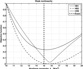
Figures (6) to (11) show the curves of the objective function over a range of values of the unknown nonlinear parameter. The exact value is indicated by the vertical line in order to facilitate the comparison with the actual minima in the curves which are the points to which an optimization algorithms are expected to converge. Moreover, the figures are divided according to the level of nonlinearity and the domain of the test, either frequency or time. The nonlinearity levels considered are obtained by applying different amplitudes of the excitation force, F = 0.1 N, 0.25 N and 1.0 N, for weak, medium and strong nonlinearity, respectively.
10 11 12 13 14 15 16 17 18 19 20
0 0.1 0.2 0.3 0.4 0.5 0.6 0.7 0.8 0.9 1
Objective function
Weak nonlinearity
Nonlinear parameter k
nl [N/m 3
]
HB1 HB2 CRE Exact
Figure 6. Evolution of the frequency residuals with the variation of the nonlinear parameter considering weak nonlinearity, where HB1 and HB2 are the residuals by using Eqs. (10) and (11), respectively.
10 11 12 13 14 15 16 17 18 19 20
0 0.1 0.2 0.3 0.4 0.5 0.6 0.7 0.8 0.9 1
Objective function
Weak nonlinearity
Nonlinear parameter k
nl [N/m 3
]
RFS1 RFS2 POD Exact
Figure 7. Evolution of the time residuals with the variation of the nonlinear parameter considering weak non-linearity, where RFS1 and RFS2 are the residuals by using Eqs. (20) and (21), respectively.
The first remark is that all curves are convex and hence well adapted to conventional local optimization procedures. The frequency methods studied here introduce in a strong linearization due the application of the HB method, once it is considered that the response of a nonlinear structure due to harmonic excitation is approximated by a harmonic function with contribution only provided by the fundamental frequency.
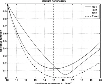
10 11 12 13 14 15 16 17 18 19 20 0
0.1 0.2 0.3 0.4 0.5 0.6 0.7 0.8 0.9 1
Objective function
Medium nonlinearity
Nonlinear parameter k
nl [N/m 3
]
HB1 HB2 CRE Exact
Figure 8. Evolution of the frequency residuals with the variation of the nonlinear parameter considering medium nonlinearity, where HB1 and HB2 are the residuals by using Eqs. (10) and (11), respectively.
10 11 12 13 14 15 16 17 18 19 20
0 0.1 0.2 0.3 0.4 0.5 0.6 0.7 0.8 0.9 1
Objective function
Medium nonlinearity
Nonlinear parameter k
nl [N/m 3
]
RFS1 RFS2 POD Exact
Figure 9. Evolution of the time residuals with the variation of the nonlinear parameter considering medium nonlinearity, where RFS1 and RFS2 are the residuals by using Eqs. (20) and (21), respectively.
In the frequency domain, the CRE gives superior results in comparison to the HB method since in this approach the FRF information on the mass 2, considered unmeasured, is estimated by solving the linear system given by Eq. (16).
In the time domain, the same can be said for the RFS method which benefits from a knowledge of a complete set of measurement points. The RFS approach also appears to be best adapted to treat all types of nonlinearities since the method is based on the exact equations. In all cases the minima of the curves correspond to the
exact value of the nonlinear parameter knl. However, it is unrealistic
to expect a complete knowledge of the system state vector as is required in this approach.
10 11 12 13 14 15 16 17 18 19 20
0 0.1 0.2 0.3 0.4 0.5 0.6 0.7 0.8 0.9 1
Objective function
Strong nonlinearity
Nonlinear parameter k
nl [N/m 3
] HB1
HB2 CRE Exact
Figure 10. Evolution of the frequency residuals with the variation of the nonlinear parameter considering strong nonlinearity, where HB1 and HB2 are the residuals by using Eqs. (10) and (11), respectively.
10 11 12 13 14 15 16 17 18 19 20
0 0.1 0.2 0.3 0.4 0.5 0.6 0.7 0.8 0.9 1
Objective function
Strong nonlinearity
Nonlinear parameter k
nl [N/m 3
]
RFS1 RFS2 Exact
Figure 11. Evolution of the time residuals with the variation of the nonlinear parameter updating considering strong nonlinearity, where RFS1 and RFS2 are the residuals by using Eqs. (20) and (21), respectively.
and then to apply the POD to each cluster in order to try to preserve the character of the nonlinear effects. This technique is known as nonlinear proper orthogonal decomposition (Kerschen, 2002).
In terms of computational costs, the frequency methods are more demanding because they require the simulation of a sinusoidal excitation over the frequency range for each iteration. The POD also requires the solution of the nonlinear equations of
motion for each value of knl. The lowest computational cost is
required by the RFS methodology.
Final Remarks
The different metrics discussed in the present paper for comparing nonlinear model updating technique have proven to be effective in working with structures with local and weak nonlinearities. However, in the case of strong nonlinearity, only the RFS method provided accurate results. Nonetheless, this approach must be adapted in order to be applied to complex structures. In perspective, further study should focus on two aspects: (1) nonlinear methods capable of accounting for strong nonlinear effects, and (2) a time domain approach based on the constitutive equation error, which should have the advantage of the RFS method without the constraint of measuring all model degrees of freedom. Moreover, in order to consider nonlinear updating in systems with strong nonlinearities and to overcome the above-mentioned difficulties, it will be fundamental to consider unconventional approaches based on adaptive filters, nonlinear state estimation, as well as other recent techniques based on the Volterra series.
Acknowledgements
The authors would like to thank the Centre National d’Etudes Spatiales, CNES – Toulouse for their generous support in this project. The authors also acknowledge the Associate Editor and the reviewers for their valuable comments.
References
Böswald, M. and Link, M., 2004, “Identification of non-linear joint parameters by using frequency response residuals”, In: International Conference on Noise Vibration Engineering, pp. 3121 – 3140.
Campello, R. J., Fávier, G. and Amaral, W. C., 2004, “Optimal expansions of discrete-time volterra models using laguerre functions”,
Automatica, Vol. 40, No. 1, pp. 815 – 822.
A. Deraemaeker, Ladevèze, P. and Leconte, Ph., 2002, “Reduced bases for model updating in structural dynamics based on constitutive relation error”, Computer Methods in Applied Mechanics and Engineering, Vol. 191, pp. 2427 – 2444.
Friswell, M. I. and Mottershead, J. E., 1995,“Finite Element Model Updating in Structural Dynamics”, Kluwer Academy Publishers.
Kerschen, G., 2002, “On the Model Validation in Non-linear Structural Dynamics”, PhD Thesis, Université de Liège, Belgium, 184 p.
Kerschen, G., Golinval, J. C. and Worden, K., 2001, “Theoretical and experimental identification of a non-linear beam”, Journal of Sound and
Vibration, Vol. 244, No. 4, pp. 597 – 613.
Kerschen, G., Worden, K., Vakakis, A. F. and Golinval, J. C., 2006, “Past, present and future of nonlinear system identification in structural dynamics”,
Mechanical Systems and Signal Processing, Vol. 20, pp. 502 – 592.
Lenaerts, V., Kerschen, G. and Golinval, J. C., 2001, “Proper orthogonal decomposition for model updating of non-linear mechanical system”,
Mechanical Systems and Signal Processing, Vol. 15, No. 1, pp. 31 – 43.
Meyer, S. and Link, M., 2003, “Modelling and updating of local non-linearities using frequency response residuals”, Mechanical Systems and
Signal Processing, Vol. 17, No. 1, pp. 219 – 226.
Puel, G., 2001, “Mise en évidence et recalage des non-linéarités locales en dynamique des structures”, Master’s thesis, Université Paris VI, France.
Schmidt, R., 1994, “Updating non-linear components”, Mechanical
Systems and Signal Processing, Vol. 8, No. 6., pp. 679 – 690.
Schultze, J. F., Hemez, F. M., Doebling, S.W. and Sohn, H., 2001, “Application of non-linear system model updating using feature extraction and parameter effect analysis”, Shock and Vibration, Vol. 8, pp. 325 – 337.
Silva, S., Dias Junior, M. and Lopes Junior, V, 2007, “Damage detection in a benchmark structure using Ar-Arx models and statistical pattern recognition”, Journal of the Brazilian Society of Mechanical Sciences and
Engineering, Vol. 29, No. 2, pp. 174 – 184.
Sohn, H., Czarnecki, J. J., Farrar, C. R., and Fellow, P. E., 2000, “Structural Health Monitoring using Statistical Process Control”, Journal of
Structural Engineering, ASCE,Vol. 126, No. 11, pp. 1356 - 1363.
Worden, K. and Manson, G. A. , 2005, “A Volterra series approximation to the coherence of the duffing oscillator”, Journal of Sound and Vibration, Vol. 286, No. 3, pp. 592 – 547.
Worden, K. and Tomlinson, G. R., 2001, Nonlinearity in Structural Dynamics. London : Institute of Physics Publishing.