NEGATIVE NON-GROUND QUERIES
IN WELL FOUNDED SEMANTICS
Facultade de Ciˆ
encias e Tecnologia
Departamento de Inform´
atica
NEGATIVE NON-GROUND QUERIES
IN WELL FOUNDED SEMANTICS
Por
V´ıctor Pablos Ceruelo
Dissertac¸ao apresentada na Facultade de Ciˆ
encias e Tecnologia
da Universidade Nova de Lisboa para obtenc¸ao do grau de
Mestre em Computational Logic
Orientador: Jos´
e J´
ulio Alves Alferes
Lisboa
The existing implementations of Well Founded Semantics restrict or forbid the use of variables when using negative queries, something which is essential for using logic programming as a programming language.
We present a procedure to obtain results under the Well Founded Semantics that removes this constraint by combining two techniques: the transformation presented in [MMNMH08] to obtain from a program its dual and the derivation procedure pre-sented in [PAP+91] to determine if a query belongs or not to the Well Founded Model of a program.
Some problems arise during their combination, mainly due to the original envi-ronment for which each one was designed: results obtained in the first one obey a variant of Kunen Semantics and non-ground programs are not allowed (or previously grounded) in the second one.
Most of these problems were solved by using abductive techniques, which lead us to observe that the existing implementations of abduction in logic programming disallow the use of variables.
The reason for that is the impossibility to evaluate non-ground queries, so it seemed interesting to develop an abductive framework making use of our negation system.
Contents . . . 5
Figures . . . 7
CHAPTER1 INTRODUCTION 9 CHAPTER2 SEMANTICS 17 2.1 Preliminaries . . . 17
2.1.1 Fixed Points . . . 23
2.2 Clark’s Predicate Completion Semantics . . . 24
2.2.1 Three-Valued Extensions . . . 26
2.2.2 Drawbacks of Clark’s Completion Semantics . . . 28
2.3 Least Model Semantics . . . 29
2.4 Perfect Model Semantics . . . 31
2.4.1 Perfect Models As Iterated Fixed Points and Iterated Least Models 36 2.4.2 Extensions of the Perfect Model Semantics . . . 38
2.5 Well Founded Model Semantics . . . 39
CHAPTER3 ON IMPLEMENTING WELL FOUNDED SEMANTICS 43 3.1 Negation as Failure . . . 45
3.2 Constructive Intensional Negation . . . 47
3.3 Derivation Procedure for Extended Stable Models . . . 51
3.4 The general picture of our implementation . . . 53
3.5 The universal quantification . . . 55
CHAPTER4 IMPLEMENTATION 59 4.1 Transform Overlapping Clauses into Nonoverlapping Ones . . . 60
4.2 Calculating the Negation of the clauses . . . 66
4.3 Adding the well founded semantics behavior . . . 71
4.3.1 Problems of loop detection . . . 80
4.4 The implementation of inequalities . . . 98
4.5 forall/2implementation . . . 102
CHAPTER5 EXTENSION: ABDUCTION 107 5.1 The theoretical approach of abduction . . . 109
5.5 Illustrative examples . . . 127 5.6 Summarizing the method of our adbuctive framework . . . 136
CHAPTER6 CONCLUSIONS 137
4.1 SLD-derivation of program 4.3.4 . . . 76
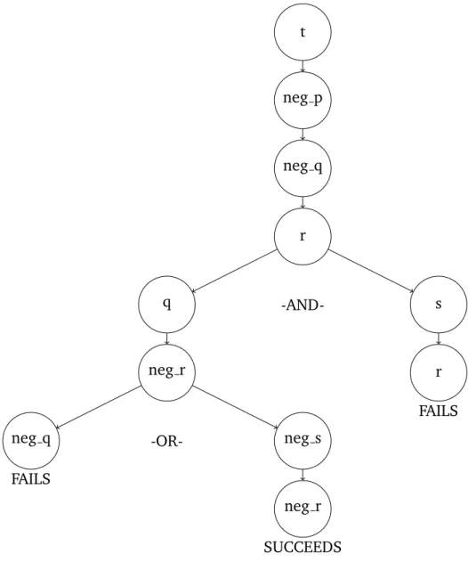
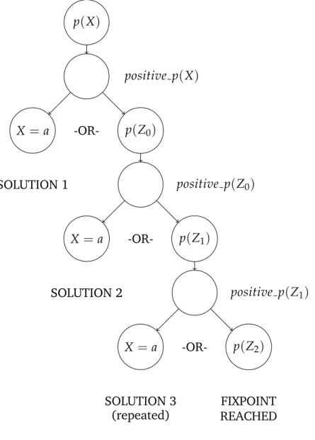
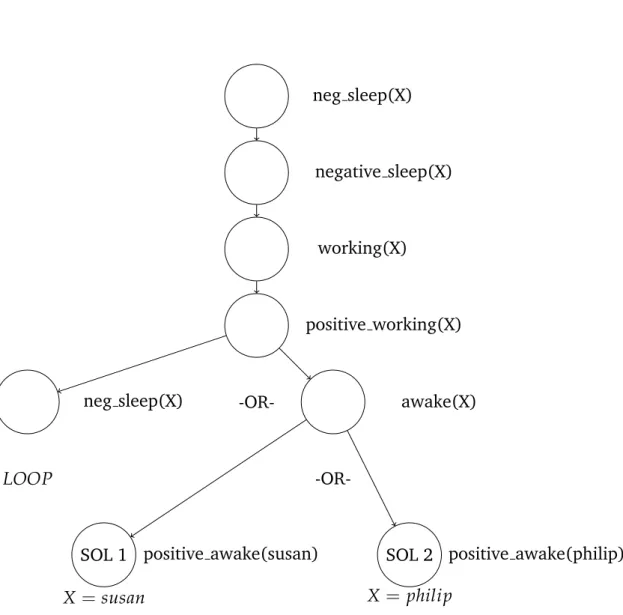
4.2 Evaluation of query?−t.in the example 1.1 from [SSW96] . . . 77
4.3 SLD-derivation of program 4.3.7 (simplified) . . . 79
4.4 SLD-derivation of program 4.3.8 . . . 82
4.5 Ideal derivation of program 4.3.8 . . . 84
4.6 SLD-derivation of program 4.3.10. . . 86
4.7 Ideal derivation of program 4.3.10. . . 87
4.8 Proposed derivation of program 4.3.12 step 1. . . 89
4.9 Proposed derivation of program 4.3.12 step 2. . . 89
4.10 Proposed derivation of program 4.3.12 step 3. . . 90
4.11 Proposed derivation of program 4.3.12 step 4. . . 90
4.12 Proposed derivation of program 4.3.12 step 5. . . 91
4.13 Proposed derivation of program 4.3.12 step 6. . . 92
4.14 Proposed derivation of program 4.3.12 step 7. . . 93
4.15 Proposed derivation of program 4.3.12 step 8 part 1 of 2. . . 94
4.16 Proposed derivation of program 4.3.12 step 8 part 2 of 2. . . 95
4.17 Proposed derivation of program 4.3.12 step 9. . . 96
I
NTRODUCTION
Kowalski and Colmerauer’s choice of the elements of first-order logic supported in logic programming was influenced by the availability of implementation techniques and efficiency considerations. Among those important aspects not included from the beginning we can mention evaluable functions, negation and higher order features. All of them have revealed themselves important for the expressiveness of logic pro-gramming as a propro-gramming language. Here we propose an implementation for Well Founded Semantics (WFS, see Sec. 2.5) that solves some pending problems with nega-tion: floundering when trying to solve non-ground negative queries
Negation in logic has been widely studied and its declarative semantics has been defined in multiple ways (see Chapter 2 for an overview). The development of the op-erational procedures for negation has been influenced by the necessity of using logic programs as programs (coding algorithms), while the development of the declarative semantics has been influenced by the purpose of using logic programs as a knowl-edge representation framework. These two different concerns lead to two different approaches to the meaning of logic programs, that we call respectively proof-theoretic approach and model-theoretic approach.
SMOD-stable models [PAP+91].
Although some authors argue that programs with contradictory, inconsistent or in-complete information are erroneous and not useful, the fact is that when representing knowledge we can not get rid of them. The following program is an example of this. Program 1.0.1
1
work ← ¬tired.
2
sleep ← ¬work.
3
tired ← ¬sleep.
4
angry ← work, ¬paid.
5
paid ← .
This program naturally encodes the knowledge that: we work if we are not tired (1), if we do not work then we sleep (2), we get tired if we do not sleep (3), when we work and we are not paid we get angry (4), and we are always paid (5).
If we try to determine if we are paid it is clear that we are, but we can not deter-mine if we work, we sleep, we are tired or we are angry. When evaluating the logic program the result is almost the same: we get an infinite loop when evaluating the querieswork,sleep,angryortired.
Depending on the point of view, we can describe our knowledge about these propo-sitions as incomplete or perhaps even confusing. The model-theoretic methods focus in assigning a truth value (undefined, false or even true) to a proposition suffering from this problems. Their proposal is to associate a model (see Def. 2.1.19) to the program and answer the queries directed to the program in accordance to this model. The model is themeaning of the program, or itsdeclarative semantics. For example, the
Well Founded Model (WFM, see Def. 2.5.2) for program 1.0.1 is { paid }, so that the atom paid belongs to the model and is thus true. Consequently, its negation, ¬paid, is false. Moreover, neither work, sleep, angry, tired nor their negations belong to our model and they are assigned theundefinedtruth value.
The definitions of the model-theoretic methods usually require that, in presence of variables, programs must be grounded before evaluating the model, and this ground-ing process might obtain an infinite ground program. This can be observed in the example program 1.0.2, where the Herbrand Universe (see Def. 2.1.9) is the infinite representation of the natural numbers: U= (0, s(0), s(s(0)), ...).
Program 1.0.2 (Peano numbers)
1
natural(0).
2
natural(s(X)) ← natural(X).
3 4
even(0).
5
even(s(X)) ← odd(X).
6
As we usually tend to program by using variables and functor symbols to build the data structures of our programs (see Def. 2.1.2), instead of computing the Herbrand Universe to determine the model (which is unfeasible for a machine), the implemen-tations rely on top-down methods for evaluating whether the query belongs or not to the model (see chapter 3). While for positive programs these methods works per-fectly, when dealing with negative non-ground queries they do not work adequately: as they make use of negation as failure they suffer from floundering. We first introduce negation as failure and just after it the floundering problem.
Negation as (finite) failure is the most common negation mechanism in logic pro-gramming. It is a meta-inference-rule allowing one to prove the negation of a ground goal, when the proof of the corresponding positive goal finitely fails. So, to prove¬a
in the following program we just have to prove thatafinitely fails. As in this case ahas a proof,¬a is not proven. On the contrary,b has no proof, and so¬bcan be proved. Program 1.0.3
1
a ← c.
2
b ← d.
3
c.
While negation as failure works perfectly for non-ground queries, when dealing with variables it produces unexpected results. In the following example, to prove ¬a(1) (which is again a ground query) we need to prove that a(1) finitely fails, and from that result negation as failure allows us to prove ¬a(1), which is the correct result. But to prove ¬a(X) we need to prove that a(X) finitely fails. As a(X) has a proof for X =2, it does not finitely fail and we get no proof for ¬a(X). So, while we expected a proof with the substitution X =1 (or, more generally, with X 6=2), what we get is “no”.
Program 1.0.4
1
a(X) ← r(X).
2
r(2).
Evaluation of queries ¬a(1) and¬a(X)in program 1.0.4 ?- ¬a(1).
yes
?- ¬a(X). no
1
friend(me, juan).
2
friend(me, pepe).
3
friend(juan, antonio).
4
friend(pepe, maria).
5
...
6
friend(X, Z) ← friend(X, Y) , friend(Y, Z).
The ones which are not my friends are then the ones that are not direct friends of me or direct friends of one of my friends. If we make a positive non-ground (or ground) query, the top-down method works perfectly, and it obtains all my friends one by one.
Evaluation of query f riend(me, X)in program 1.0.5
?- friend(me, X). X = juan ? ; X = pepe ? ; X = antonio ? ; X = maria ? ; ...
Correct results are also guaranteed if we make a ground negative query. But if we make a negative non-ground query, before getting any result the first thing that the method will do is to determine which are my friends. As the set of my friends behaves like an infinite set, it is impossible to compute the whole set of friends.
The existing WFS implementations do not have a correct management of univer-sally quantified variables and use basic methods that suffer from floundering1 (Both examples 1.0.4 and 1.0.5 suffer from floundering, although the end of the computa-tion in the second one presents an error, usuallyOutOfMemoryexception).
The main objective of this work is to develop an implementation dealing correctly with non-ground queries under the Well Founded Semantics. Non ground queries in logic programming is solved in the negation system developed in
[MHMN00, MHMNH01, MH03, MMNMH08], where the authors incorporate nega-tion in the Prolog system Ciao [Bue95]. They developed a system able to manage negation properly, combining different techniques and using static and dynamic tests to determine which method is the best in each case. They are able to select the built-in negation as failure(NAF, see Sec. 3.1) when a groundness analysis tells that every negative literal is ground at call time, select Finite Constructive Intensional Negation (an improved version of Constructive Intensional Negation that only works for finite domains) when the analysis tells that the program has no infinite answers, or using Constructive Intensional Negation (see Sec. 3.2) in the worst case.
Despite the huge amount of work done, the authors developed the system under a variant of Clark’s Predicate Completion Semantics (see Sec. 2.2) that they suggest
1When the evaluation stops with no answer the problem is called floundering. This problem has
to be seen as a CLP version of Kunen’s semantics (KS, see Sec. 3.2). The drawback of Kunen’s Semantics, as other proof-theoretic methods, is that it does not work ade-quately in presence of contradictory, inconsistent or incomplete information.
In this thesis we generalize this work on Constructive Intensional Negation [MMNMH08] to answer (non-ground) queries under the Well Founded Semantics. This is done by combining the procedure used in [MMNMH08] with the one used in [PAP+91].
Basically, we take from [MMNMH08] the methods to calculate the dual program, and the derivation procedure from [PAP+91]. As the derivation procedure was not developed to deal with dual programs, it is modified to take into account the following characteristics that dual programs present:
1. the dual of a unification is a disequality. Since the predefined inequal-ity predicate in logic programming is not suitable for dealing with variables (see Sec. 4.4), in the implementation we must use attributed variables (see Def. 4.4.1) to deal with them.
2. if a predicate in the original program has a free variable, its negation has this variable universally quantified (see Sec. 3.5). As logic programming does not have a predefined predicate to determine if a universal quantification holds or not, we must implement a method capable of determining that.
When solving these problems we found that the techniques used resemble abduc-tive techniques (see chapter 5). In fact, abduction collects solutions and tests these solutions for the consistency of the result. Our implementation behaves like that in two parts:
1. inequalities implementation: we collect all the disequalities over a variable and finally we test if their conjunction is consistent or not (see Sec. 4.4).
2. universally quantified variables implementation: the results for the variable are collected and finally they are tested in order to find a tautology that guarantees the universal quantification to hold (see Secs. 3.5 and 4.5).
The extension of our work presented in chapter 5, abduction, comes indeed from its previous use to solve these problems: as abduction is used to solve them, the appli-cation of our negation system to abduction, in order to obtain explanations to nega-tive hypotheses, seemed rather promising. The result from applying it is an abducnega-tive framework that benefits from this new implementation of negation, and that can make an unrestricted use of variables.
One extra feature that we considered mandatory for our negation system is that solutions must be obtained in a Prolog way, i.e. one by one. In [MMNMH08], instead, the solutions returned when making a query follow the structure
sol 1∨sol 2∨. . .∨sol n ? ;
• results obtained can not be used from other Prolog programs without a previous conversion.
• one might be only interested in one solution (or a small subset of solutions), in which case it makes no sense to wait for computing the whole disjunction. This is specially important if our set of solutions has an exponential size, as may happen when the computation of the universal quantification is involved.
• if the number of solutions is infinite then computing them (or their disjunction) is unfeasible. While there is a solution, their method is not able to obtain any solution at all.
Desirably, this should be substituted by the Prolog way, so that instead of results joined by disjunction what we get is one result (disjunct) at a time, following the structure
sol 1 ? ;
sol 2 ? ; . . .
sol n ? ;
no
The implementation of the Well Founded Semantics that we finally present here, and that constitutes the main contribution of this thesis, has the following character-istics:
1. It can be applied to any kind of logic program in which no symbols are intro-duced to constraint the normal execution of Prolog, like cuts (the term ”!” ). So, no restriction exists on the use of variables in the program or in the queries. 2. Solutions are obtained one by one. Some solutions represent disequalities, and
they use attributed variables for that purpose. Disequalities are only joined if they need to be fulfilled at the same time (and only by conjunction), so they represent only one valid solution.
3. The way inequalities between variables are tested is based on abductive tech-niques: inequality conditions are assumed in advance and stored in the attribute of the variables, being really tested when the variable is bound.
4. The way that the universal quantification is evaluated uses again abductive tech-niques: solutions to the universally quantified variables are collected and tested in order to build a tautology, so it can be determined if the universal quantifica-tion holds.
5. Answers are given according to the Well Founded Semantics.
S
EMANTICS
According to [PP90], which we follow for this overview, the declarative semantics SEM(Π) of a logic program Π can be specified in various ways, among which the following two are most common. One that can be called proof-theoretic, associates with Π its first order completion COMP (Π) (e.g., COMP (Π) can be Π itself or the Clark predicate completion comp(Π) ofΠ). A formula V is said to be implied by the semantics SEM(Π) if and only if it is logically implied by the completion
COMP (Π)|=V;
i.e., if V is satisfied in all 2-valued (Herbrand or not) models of COMP (Π).
Another method of defining the declarative semantics SEM(Π) of a program is model-theoretic. The semantics is determined by choosing a set MOD(Π) of intended models of Π (in particular, one intended modelMΠ). For example, MOD(Π) can be the set of all minimal models of Π or the unique least model of Π. A formula V is said to be implied by the semantics SEM(Π) if and only if it is satisfied in all intended models:
MOD(Π) |=V (in particular,MΠ |=V):
Observe, that the proof-theoretic approach can be viewed as a special case of the model-theoretic approach. Other approaches to defining the declarative semantics are possible, e.g., a combination of proof-theoretic and model-theoretic methods has been used in [Kun87, Fit85].
2.1
Preliminaries
Definition 2.1.1 (Alphabet). By an alphabet A of a first order language Lwe mean a (finite or countably infinite) set of constant, predicate and function symbols. In addition, any alphabet is assumed to contain a countably infinite set of variable symbols, connec-tives (∨,∧,¬,←), quantifiers (∃,∀) and the usual punctuation symbols. Moreover, we assume that our language also contains propositionst, uand f, denoting the properties of being true, undefined or false.
Definition 2.1.2(Term, Functor). Terms are as customarily defined in logic:
• A variable or constant is a term.
• A function symbol (or functor) with terms as arguments is a term.
Terms may also be viewed as data structures of the program, with function symbols serv-ing as record names. The word ground is used as a synonym for “variable-free”, in keepserv-ing with common practice. Often a constant is treated as a function symbol of arity zero.
Definition 2.1.3(Predicate, Atomic Formulae, Atom). A predicate is a relation between terms, so the arguments of a predicate are terms. We use the same symbol, e.g., p, to refer both a predicate and its relation.
If p is a predicate symbol of arity n (n ≥0) and t1, ...tn are terms then p(t1, ...tn) is
an atomic formulae or atom. Predicates of arity zero are also called propositions.
Definition 2.1.4(Formulae). If F1 andF2are formulas then so are
• ¬F1
• F1∨F2
• F1∧F2
• F1 ←F2
If Xis a variable and Fis a formulae then ∃X.Fand∀X.F are formulas too. We say that X is existentially quantified in∃X.F and universally quantified in∀X.F.
Definition 2.1.5 (Quantifier-free formulae). If F is a quantifier-free formulae, then by its ground instance we mean any ground formulae obtained from F by substituting ground terms from the Herbrand UniverseU(see Def. 2.1.9) for all variables.
Definition 2.1.6 (Universal closure of a formulae). For a given formulae F of a lan-guageLits universal closure or just closure∀Fis obtained by universally quantifying all variables inFwhich are not bound by any quantifier.
Definition 2.1.7 (Expression, Sentence). An expression is a term or a formulae. A formulae with no free (unquantified) variables is a sentence.
Definition 2.1.8(Literal). A literal L is either an atom A or its negation¬A. In the first form it is called positive literal and in the second one negative literal.
Definition 2.1.9 (Herbrand Base, Herbrand Universe). The set of all ground atoms of an alphabet A is called the Herbrand Base H of A. The set of all ground terms of A is called the Herbrand UniverseUofA.
Definition 2.1.10(Logic Rule or Clause). A rule or a clause C is a formulae of the form H ← L1 ∧ ... ∧ Ln
where H is an atom other than false and{ L1, ..., Ln }is a possibly empty set of literals.
The head or conclusion H is written on the left, and its subgoals (body) if any to the right of the symbol←, which may be read “if”. In some parts of this document we refer to the head by the left hand side (lhs) of the clause, and to the body by the right hand side (rhs) of the clause.
Conforming to a standard convention, conjunction is replaced by commas and there-fore clauses are simply written in the form
H ← L1, ..., Ln
For example,
p(X) ←a(X),¬ b(X),¬ (c(X), d(X))
is a rule in which p(X) is the head, a(X) is a positive subgoal and b(X) and (c(X), d(X)) are negative subgoals. The head of a rule is always a positive literal.
Definition 2.1.11 (Logic Program (I)). By a logic program Π we mean a finite set of logic rules or clauses. IfΠis a logic program then, unless stated otherwise, we will assume that the alphabetA used to write Πconsists precisely of all the constant, predicate and function symbols that explicitly appear inΠand thusA=AΠ is completely determined1 by the program Π. We can then talk about the first order language L = LΠ of the programΠand the Herbrand base H=HΠ of the program.
Remark. Although some authors distinguish between general logic programs and normal logic programs (see [GRS91, Llo87]), we will use logic programs to refer all of them.
Definition 2.1.12 (Logic program (II)). Programs are constructed from a signature Σ =hFSΣ,PSΣi of function and predicate symbols. Provided a countable set of variables V the setTerm(FSΣ,V)of terms is constructed in the usual way.
Remark. This definition is equivalent to the previous one, but instead of defining the alphabet from the program it defines the program from the alphabet. It is used in the explanation of the Constructive Intensional Negation method (see Sec. 3.2).
Definition 2.1.13 (Horn Rule and Horn Logic Program). A horn rule is a general rule with no negative subgoals, and a Horn logic program is one only with Horn rules.
Definition 2.1.14 ((Herbrand) constraint). A (Herbrand) constraint is a first-order formula where the only predicate symbol is the binary equality operator=/2. A formula
¬(t1 = t2) will be abbreviated t1 6= t2. The constants t (for true) and f (for false)
will denote the neutral elements of conjunction and disjunction, respectively. A tuple
(x1, . . . ,xn) will be abbreviated by x. The concatenation of tuples x and y is denoted
x·y.
Definition 2.1.15 ((constrained) Horn clause). A (constrained) Horn clause is a for-mula
h(x) ← b1(y·z), . . . , bn(y · z) []c(x·y)
where x, y and z are tuples from disjoint sets of variables.2 The symbols “,” and “[]” act here as aliases of logical conjunction (the second one is introduced for readability of the examples).
Definition 2.1.16((constrained) program). A (constrained) program is: p(x) ← B1(y1·z1) []c1(x·y1)
.. .
p(x) ←Bm(ym·zm) []cm(x·ym)
The set of defining clauses for predicate symbolpin programΠis denoteddefΠ(p). With-out loss of generality we have assumed that the left hand sides indefΠ(p)are syntactically identical.
Definition 2.1.17(Completed definition of a program). Assuming the normal form, let defΠ(p) = {p(x) ← Bi(yi·zi)[]ci(x·yi)|i ∈ 1 . . .m}. The completed definition of p,
cdefΠ(p)is defined as the formula
∀x.
"
p(x) ⇐⇒ m _
i=1
∃yi. ci(x·yi)∧ ∃zi.Bi(yi·zi)
#
Definition 2.1.18(Interpretation). By a 3-valued Herbrand interpretationI of the lan-guageLwe mean any pair<T, F >, whereTandFare disjoint subsets of the Herbrand
baseH. The setTcontains all ground atoms true inI, the setFcontains all ground atoms false in I and the truth value of the remaining atoms inU = H−(T∪F) is undefined. We assume that in every interpretationIthe propositiontis true, the propositionfis false and the propositionuis undefined. A 3-valued interpretation I is 2-valued if all ground atoms (except for the propositionu) are either true or false inI.
An alternative way to represent an interpretation I =<T, F>is
I = T ∪ {¬L | L ∈ F}.
Definition 2.1.19(Model). Mis a model of a programΠif and only if the degree of the truth of the head of every clause is at least as high as the degree of truth of its body. To use this definition we need to introduce how to evaluate the degree of truth of the head and the body of the clauses.
Any interpretationI=<T, F>can be equivalently viewed as a function
I : H → { 0, 12, 1}, from the Herbrand base Hto the 3-element setV ={ 0, 12, 1 }, defined by:
I(A) =
0, i f A∈ F
1
2, i f A∈ U
1, i f A∈ T
2The notationp(x)expresses thatVars(p(x))∈x, not that it is identical top(x
We now extend the function (interpretation) I : H → V recursively to the truth valuationˆI: C→Vdefined on the setCof all closed formulae of the language.
[Prz89a] If I is an interpretation, then the truth valuationˆI corresponding to I is a functionIˆ: C→Vfrom the set C of all (closed) formulae of the language toVrecursively defined as follows:
• If A is a ground atom, thenˆI(A) = I(A).
• If S is a closed formulae thenˆI(¬S) =1−ˆI(S).
• If S and T are closed formulae, then
ˆ
I(S∧T) =min{ˆI(S), ˆI(T)}; ˆ
I(S∨T) = max{ˆI(S), ˆI(T)};
ˆ
I(T ←S) =
1, i f ˆI(T)≥ˆI(S)
0, otherwise
• For any formulae S(X) with one unbounded variable X:
ˆ
I(∀X.S(X)) = min{Iˆ(S(A)): A ∈HΠ };
ˆ
I(∃X.S(X)) =max { Iˆ(S(A)) : A∈ HΠ };
where the maximum (resp. minimum) of an empty set is defined as 0 (resp. 1).
Once introduced how to evaluate the truth values of the head and the body of a clause we can expose that if our program is a set of rules of the form A ← L1, ..., Lm, where
m ≥ 0, A’s is an atom and Li’s are literals, then an (Herbrand) interpretation M is a model of a program Π if all the program clauses are true in M, i.e., if for every ground instance of a program clause we have
ˆ
M(A) ≥ min{ Mˆ(Li): i ≤ m }
Thus,M is a model of a program Π if and only if the degree of the truth of the head of every clause is at least as high as the degree of truth of its body, as told before. By a ground instantiation of a logic program Π we mean the (possibly infinite) theory consisting of all ground instances of clauses fromΠ.
Corollary 2.1.1. An (Herbrand) interpretationMis a model of a programΠif and only if it is a model of its ground instantiation.
A program Πcan have different Herbrand models, as can be seen in the following example. In fact, programs with negation may have several minimal Herbrand models.
Example 2.1.1 (Program with different Herbrand models)
1
p(1).
2
q(2).
3
model 1: {p(1), q(1), q(2)}
model 2: {p(1), p(2), q(1), q(2)}
Models are usually associated with programs to represent the “meaning of the program” or its “declarative semantics”. The idea is that a declarative semantics for a class of logic programs can be defined by selecting, for each program Πin this class, one of its models to determine which answer to a given query is considered correct. For instance, a query without variables should be answered “yes” if it belongs to the model and no otherwise, and a query with variables should be answered “yes” if by substitution we found a ground version of the query that belongs to the model.
Ideally we should be able to select a canonical model for that purpose, but instead of that we have different approaches to select it, as Stable Models [GL88], Perfect Models [Prz88] and Well Founded Models (WFM) [GRS91, VGRS88]. Each one of them is linked with a semantics, which respectively are Stable Model Semantics (SMS) [GL88], Perfect Model semantics (PMS) [Prz88, ABW88, vG89], and Well Founded Semantics (WFS) [GRS91, VGRS88]. A survey on PMS and WFS is exposed in the following sections. We refer the reader to [GL88, PP90] for a survey on SMS.
Definition 2.1.20. [Prz89a] If Iand Jare two interpretations then we say that I4J if I(A) ≤ J(A)(or,equivalently, ˆI(A) ≤ Jˆ(A))
for any ground atom A. IfIis a collection of interpretations, then an interpretation I∈ I
is called minimal inI if there is no interpretation J ∈ Isuch that J 4I and J 6= I. An interpretation I is called least in I if I 4J, for any other interpretation J ∈ I. A model M of a theory R is called minimal (resp. least) if it is minimal (resp. least) among all models of R.
Proposition 2.1.1. If I =< T,F > and I′ =< T′,F′ > are two interpretations, then
I4I’ iff T ∈ T′andF ∈ F′. In particular, for 2-valued interpretations, I4I’ iff I∈I’.
Thus I 4 I’ if and only if I has no more true facts and no less false facts than I’ .
This means that minimal and least models of a theory R minimize the degree of truth of their atoms, by minimizing the set T of true atoms and maximizing the set F of false atoms F. In particular, the least interpretation in the set of all interpretations is given by I=<∅,H >.
As we mentioned above, [Fit85] considers a different ordering of truth values based on the degree of information rather than on the degree of truth. Under this ordering, the ‘unknown’ value is less than both values ‘true’ and ‘false’, with ‘true’ and ‘false’ being incompatible. This immediately leads to a different ordering between interpretations and to different notions of minimal and least models.
Definition 2.1.21. [Fit85] If I =< T,F >and I’=< T′,F′ >are two interpretations,
then we say that I 4F I’ iff T ⊆T’ and F ⊆F’. We call this ordering the F-ordering. If I
In particular, the F-least interpretation in the set of all interpretations is given by I =< ∅,∅ >. The notions of F-minimal and F-least models are different from the
notions of minimal and least models (see 2.1.20). While minimal and least models of a theory R minimize the degree of truth of their atoms, by minimizing the set T of true atoms and maximizing the set F of false atoms F, F-minimal and F-least models minimize the degree of information of their atoms, by jointly minimizing the sets
T and F of atoms which are either true or false and thus maximizing the set U of unknown atoms. For example, the F-least model of the program p ← p is obtained when p is undefined, while the least model of Π is obtained when p is false. As it will be seen in the sequel, this distinction reflects fundamental differences between the semantics based on Clark’s completion and model-theoretic semantics, such as the least model semantics, perfect model semantics or well-founded semantics.
2.1.1
Fixed Points
Declarative semantics of logic programs is often defined using fixed points of some natural operatorsΨacting on ordered sets of interpretations. Suppose≤is an order-ing on the setI of interpretations of a given language, J is a subset of I and Ψ is an operatorΨ: I→IonI.
Definition 2.1.22. The operator Ψ is called monotone if I ≤ J implies Ψ(I) ≤ Ψ(J), for any I, J ∈ I. An interpretation I∈ Iis a fixed point of Ψif Ψ(I) = I . By the least upper bound∑JofJ(resp. the greatest lower boundΠJofJ) we mean an interpretation I∈ Isuch that J≤I , for any J ∈Jand J ≤J’ for any other J’ with this property (resp. I ≤ J , for any J ∈ J and J’ ≤ J for any other J’ with this property). By the smallest interpretation (under the given ordering) we mean an interpretation I0 such that I0 ≤I,
for any other interpretation I.
Least fixed points of monotone operators Ψ are often generated by iterating the operator Ψ starting from the smallest interpretation I0 and obtaining the (possibly transfinite) sequence:
Ψ↑0= I 0;
Ψ↑α+1=Ψ(Ψ↑α); Ψ↑λ =∑α<λΨ↑α;
for limit ordinalsλ. Clearly, an iterationΨ↑α is a fixed point ofΨif and only if
Ψ↑α =Ψ↑α+1.
In the sequel we will consider two principal orderings among interpretations, namely the standard ordering 4 (see Def. 2.1.20) and the F-ordering 4F (see Def. 2.1.21). Operators acting on sets of interpretations ordered by the standard ordering, will be denoted by Ψ or Θ, while those acting on sets of interpretations ordered by the F-ordering, will be denoted by Φ or Ω. Recall that I0 =< ∅,H >
(resp. I0 =<∅,∅ >) is the smallest (resp. F-smallest) interpretation in the set of all interpretations ordered by4(resp. 4F ).
(resp. ΠFJ) the least upper bound (resp. the greatest lower bound) ofJ with respect to4F.
Observe, that ifJ ={Js : s∈ S}, with Js =<Ts;Fs >, then:
∑J=< S
s∈S
Ts, T s∈S
Fs >;
ΠJ=< S
s∈S
Ts, T s∈S
Fs >;
∑FJ=< S
s∈S
Ts, S s∈S
Fs >;
ΠFJ=< T
s∈S
Ts, T s∈S
Fs >.
Although∑J,ΠJandΠFJare always well-defined interpretations,∑F J =< T, F >
may not be an interpretation, because the setsTand F may not be disjoint. However,
∑FJis always an interpretation, provided thatJis an F-directed set of interpretations, i.e., such that for any J, J’∈ Jthere is a J”∈ Jsatisfying J4F J” and J’4F J”.
2.2
Clark’s Predicate Completion Semantics
The most commonly used declarative semantics of logic programs, although less pop-ular in the context of knowledge representation, is based on the so called Clark predi-cate completion comp(Π) of a logic programΠ[Cla78, Llo87]. Clark’s completion of
Πis obtained by first rewriting every clause inΠ of the form: q(K1, ..., Kn ) ←L1 , ..., Lm,
where q is a predicate symbol and K1, ..., Kn are terms containing variables X1, ..., Xk, as a clause
q(T1, ..., Tn)←V, where Ti ’s are variables,
V =∃X1, ..., Xk (T1= K1 ∧... Tn = Kn ∧L1∧ ... ∧ Lm)
and then replacing, for every predicate symbol q in the alphabet, the (possibly empty3) set of all clauses
q(T1, ..., Tn)←V1 ...
q(T1, ..., Tn) ←Vs
with q appearing in the head, by a single universally quantified logical equivalence q(T1, ..., Tn)↔V1 ∨ ... ∨ Vs.
3If there are no clauses involving the head q(T
1, ..., Tn), then the corresponding disjunction is empty
Finally, the obtained theory is augmented by the so called Clark’s Equality Axioms (see Def. 2.2.1), which include unique names axioms and axioms for equality. These axioms are essential when considering non-Herbrand models of Clark’s completion. Definition 2.2.1 (Clark’s Equational Theory (CET)). The so called Clark’s Equality Axioms [Kun87] are:
CET1 X =X;
CET2 X =Y ⇒Y= X;
CET3 X =Y∧Y=Z ⇒X =Z;
CET4 X1 = Y1∧. . .∧Xm = Ym ⇒ f(X1, . . . ,Xm) = f(Y1, . . . ,Ym), for any
function f;
CET5 X1 = Y1∧. . .∧Xm = Ym ⇒ ( p(X1, . . . ,Xm) ⇒ p(Y1, . . . ,Ym) ), for
predicate p;
CET6 f(X1, . . . ,Xm) 6= g(Y1, . . . ,Yn), for any two different function symbols f
and g;
CET7 f(X1, . . . ,Xm) = f(Y1, . . . ,Ym) ⇒ X1 = Y1∧. . .∧Xm = Ym, for any
function f;
CET8 t[X]6=X, for any termt[X] different from X, but containing X.
Remark. The first five axioms describe the usual equality axioms and the remaining three axioms are called unique names axioms or freeness axioms. The significance of these axioms to logic programming is widely recognized [Llo87, Kun87]. The equality axioms (CET1) - (CET5) ensure that we can always assume that the equality predicate “=” is interpreted as identity in all models. Consequently, in order to satisfy the CET axioms, we just have to restrict ourselves to those models in which the equality predicate when interpreted as identity satisfies the unique names axioms (CET6) -(CET8).
Clark’s approach is mathematically elegant and founded on a natural idea that in common discourse we often tend to use ‘if’ statements, when we really mean ‘iff’ statements. For example, we may use program 2.2.1 to describe natural numbers. Program 2.2.1 (Peano numbers)
1
natural_number (0).
2
natural_number (succ(X)) ← natural_number (X).
natural number (T)↔ ∃X (T = 0∨ (T = succ(X)∨ natural number(X))) which is in fact Clark’s completion of program 2.2.1 and it indeed implies
¬natural number(MickeyMouse).
Unfortunately, Clark’s predicate completion semantics has some serious drawbacks. One of them is the fact that Clark’s completion is often inconsistent, i.e., it may not have any 2-valued (Herbrand or not) models, in which case Clark’s semantics is un-defined. For example, Clark’s completion of the program p ← ¬p is p ↔ ¬p, which is inconsistent. The situation can be even worse, e.g., Clark’s completion of the pro-gram 2.2.2 is propro-gram 2.2.3,
Program 2.2.2
1
p ← ¬q, ¬p
Program 2.2.3
1
p ← ¬q, ¬p
2 ¬q
which is inconsistent. However, after adding to program 2.2.2 a ‘meaningless’ clause q its completion becomes:
1
p ↔ ¬q, ¬p
2
q ↔ q
which has a unique 2-valued model in which q is true and p is false. On the other hand, after adding toΠanother ‘meaningless’ clause p p its completion becomes:
p↔p∨ (¬q∧ ¬p)
¬q
which has a unique, yet different, 2-valued model in which q is false and p is true.
2.2.1
Three-Valued Extensions
[Fit85] showed that the inconsistency problem for Clark’s semantics, as well as some other related problems, can be elegantly eliminated by considering 3-valued Herbrand models of the Clark predicate completion comp(Π), rather than 2-valued models only. Theorem 2.2.1 (Theorem 6.1 [Fit85]). Clark’s completion comp(Π) of any logic pro-gramΠalways has at least one 3-valued Herbrand model. Moreover, among all 3-valued models of comp(Π) there is exactly one F-least modelMΠ.
Definition 2.2.2(Fitting’s Semantics). [Fit85] Fitting’s 3-valued extension of the Clark predicate completion semantics is the semantics determined by the unique intended model MΠ or, equivalently, by the set MOD(Π) of intended models, consisting of all 3-valued Herbrand models of comp(Π).
For example, the program 2.2.2 defined before has a unique 3-valued model in which q is false and p is undefined. Fitting also provided an elegant fixed-point char-acterization of 3-valued models of comp(Π).
Definition 2.2.3 (The Fitting Operator). [Fit85] Suppose that Π is a logic program. The Fitting operatorΦ : I→Ion the setIof all 3-valued interpretations of comp(Π) is defined as follows. If I ∈Iis an interpretation of comp(Π) and A is a ground atom then Φ(I) is an interpretation given by4:
(i) Φ(I)(A) = 1 if there is a clause A ← L1, ..., Ln in Π such that I(Lˆ i) = 1, for all
i≤n;
(ii) Φ(I)(A) = 0 if for every clause A ← L1, ..., Ln in Π there is an i ≤ n such that
ˆ
I(Li) = 0;
(iii) Φ(I)(A) = 12 , otherwise.
Theorem 2.2.2. [Fit85] An interpretation I of comp(Π) is a model of comp(Π) if and only if it is a fixed point of the operatorΦ. In particular, MΠ is the F-least fixed point of Φ.
Moreover, the model MΠ can be obtained by iterating the operator Φ, namely, the sequenceΦ↑α of iterations5 ofΦ is monotonically increasing and it has a fixed point
Φ↑λ =MΠ.
Kunen [Kun87] showed that the set of formulae implied by Fitting’s semantics is not recursively enumerable and he proposed the following modification of Fitting’s approach.
Definition 2.2.4(Kunen’s Semantics). [Kun87] Kunen’s 3-valued extension of the Clark predicate completion semantics is the semantics determined by the set MOD(Π) of in-tended models, consisting of all 3-valued (Herbrand or not) models of comp(Π).
Kunen showed that his semantics is recursively enumerable and closely related to the Fitting operatorΦ.
Theorem 2.2.3. [Kun87] A closed formula V is implied by Kunen’s 3-valued extension of the Clark predicate completion semantics if and only if it is satisfied in at least one finite iteration Φ↑n of the Fitting operator Φ, n = 0,1,2, ... . Moreover, the set of formulae
implied by this semantics is recursively enumerable.
It is easy to see that Fitting’s semantics is stronger than Kunen’s semantics, i.e., any closed formula implied by Kunen’s semantics is also implied by Fitting’s semantics.
4According to the conventions adopted in Sec. 2.1,Πis assumed to be instantiated and
interpreta-tions are viewed as 3-valued funcinterpreta-tions.
5According to the convention from Sec. 2.1.1,Φis defined on the F-ordered set of interpretations
2.2.2
Drawbacks of Clark’s Completion Semantics
Unfortunately, Clark’s predicate completion does not always result in a satisfactory semantics. For many programs, it leads to a semantics which appears too weak. This problem applies both to standard Clark’s semantics as well as to its 3-valued extensions and it has been extensively discussed in the literature (see e.g. [She88, She84, Prz89b, GRS91] ). We illustrate it on the following three examples.
Example 2.2.1 Suppose that to the program 2.2.1 defined before we add a seem-ingly meaningless clause:
natural number(X) ←natural number(X). to obtain the program 2.2.4.
Program 2.2.4
1
natural_number(0).
2
natural_number(succ(X)) ← natural number (X).
3
natural_number(X) ← natural_number(X).
It appears that the newly obtained program 2.2.4 should have the same semantics. However, Clark’s completion of the new program 2.2.4 is:
natural number(T) ↔
(natural number(T) ∨T = 0∨∃X. (T = succ(X)∧natural number(X)))
from which it no longer follows that MickeyMouse (or anything else, for that matter) is not a natural number.
Example 2.2.2 (Van Gelder) Suppose, that we want to describe which vertices in a graph are reachable from a given vertex a. We could write the program 2.2.5. Program 2.2.5
1
edge(a, b)
2
edge(c, d)
3
edge(d, c)
4
reachable(a)
5
reachable(X ) ← reachable(Y), edge(Y, X).
We clearly expect vertices c and d not to be reachable. However, Clark’s completion of the predicate ‘reachable’ gives only
reachable(X)↔(X = a ∨ ∃Y (reachable(Y )∧ edge(Y, X )))
Example 2.2.3 Suppose the following program: Program 2.2.6
1
bird(tweety)
2
fly(X) ← bird(X), ¬abnormal(X)
3
abnormal(X) ← irregular(X)
4
irregular(X) ← abnormal(X).
The last two clauses merely state that irregularity is synonymous with abnormality. Based on the fact that nothing leads us to believe that tweety is abnormal, we are justified to expect that tweety flies, but Clark’s completion of program 2.2.6 yields
fly (T)↔(bird(T)∨ ¬abnormal(T)) abnormal(T) ↔irregular(T),
from which it does not follow that anything flies. On the other hand, without the last two clauses (or without just one of them) Clark’s semantics produces correct results.
The above described behavior of Clark’s completion is bound to be confusing for a thoughtful logic programmer, who may very well wonder why, for example, the ad-dition of a seemingly harmless statement “natural number(X)←natural number(X)” should change the meaning of the first program. The explanation that will most likely occur to him will be procedural in nature, namely, the fact that the above added clause may lead to a loop. But it was the idea of replacing procedural programming by declarative programming, that brought about the concept of logic programming and deductive databases in the first place, and therefore it seems that such a procedural explanation should be flatly rejected.
Some of the problems mentioned above are caused by the difficulties with the rep-resentation of transitive closures when using Clark’s semantics (e.g., in the program 2.2.5). [Kun87] formally showed that Clark’s semantics is not sufficiently expres-sive to naturally represent transitive closures. In the following sections we discuss model-theoretic approaches to declarative semantics of logic programs which attempt to avoid the drawbacks of Clark’s semantics discussed above.
2.3
Least Model Semantics
The model-theoretic approach is particularly well-understood in the case of positive logic programs. In this section we assume that all interpretations are 2-valued.
Example 2.3.1 Suppose that our program Π (taken from [PP90]) consists of clauses:
Program 2.3.1
1
able mathematician(X) ← physicist(X).
2
physicist(einstein).
3
This program has several different models, the largest of which is the model in which both Einstein and Iacocca are at the same time businessmen, physicists and good mathematicians. This model hardly seems to correctly describe the intended meaning of Π. Indeed, there is nothing in this program to imply that Iacocca is a physicist or that Einstein is a businessman. In fact, we are inclined to believe that the lack of such information indicates that we can assume the contrary.
The program also has the unique least model MΠ :
{physicist(einstein), businessman(iacocca), able mathematician(einstein)}, in which only Einstein is a physicist and good mathematician and only Iacocca is a businessman. This model seems to correctly reflect the semantics of P, at the same time incorporating the classical case of the closed-world assumption [Rei77] if no reason exists for some positive statement to be true, then we are allowed to infer that it is false. It turns out that the existence of the unique least modelMΠ is the property shared by all positive programs.
Theorem 2.3.1. [vEK76b] Every positive logic programΠhas a unique least (Herbrand) modelMΠ.
This important result led to the definition of the so called least model semantics for positive programs.
Definition 2.3.1(Least Model Semantics). [vEK76b] By the least model semantics of a positive programΠwe mean the semantics determined by the least Herbrand modelMΠ ofΠ.
The least Herbrand model semantics is very intuitive and it seems to properly reflect the intended meaning of positive logic programs. The motivation behind this approach is based on the idea that we should minimize positive information as much as possible, limiting it to facts explicitly implied by Π, and making everything else false. In other words, the least model semantics is based on a natural form of the closed world assumption.
The least model semantics avoids the drawbacks of the Clark predicate completion discussed in the previous section. For example, the least Herbrand modelMΠ of the programs 2.2.1 and 2.2.4 given above is:
{natural number(0), natural number(succ(0)), natural number(succ(succ(0))), ...}
which is exactly what we intended. Similarly, the least Herbrand model MΠ of the program 2.2.5 above is:
{edge(a, b), edge(c, d), edge(d, c), reachable(a), reachable(b)}, which is again exactly what we would expect.
Least model semantics also has a natural fixed point characterization. First we define the Van Emden-Kowalski immediate consequence operatorΨ:I→Ion the set
Definition 2.3.2(The Van Emden-Kowalski Operator). [vEK76b] Suppose that Π is a positive logic program, I∈ Iis an interpretation ofΠand A is a ground atom. ThenΨ(I) is an interpretation given by:
(i) Ψ(I)(A) = 1 if there is a clause A ← A1, ...,An in Π such that I(Ai) = 1, for all
i≤n;
(ii) Ψ(I)(A) = 0 , otherwise.
Theorem 2.3.2. [vEK76b] The Van Emden-Kowalski operatorΨhas the least fixed point, which coincides with the least modelMΠ. Moreover, the model MΠ can be obtained by iteratingω times the operatorΨ, namely, the sequenceΨ↑n,
n = 0, 1, 2, ...,ω, of iterations6
of Ψis monotonically increasing and it has a fixed point Ψ↑ω =MΠ.
The least model semantics is strictly stronger than Clark’s semantics:
Theorem 2.3.3. Suppose thatΠis a positive logic program. If a closed formula is implied by the Clark predicate completion semantics (or by one of its 3-valued extensions) then it is also implied by the least model semantics.
The only serious, drawback of the least model semantics seems to be the fact that it is well defined for a very restrictive class of programs. Programs which are not positive, in general, do not have least models. For example, the program p ← ¬ q
has two minimal models{p}and{q}, but it does not have the least model. Similarly, the program 2.2.6 from Example 2.2.3 does not have the least model.
2.4
Perfect Model Semantics
As we have seen above, although the least model semantics seems suitable for the class of positive programs, it is not adequate for more general programs, allowing negative premises in program clauses. The inclusion of negation in program clauses increases the expressive power of logic programs and thus is of great practical impor-tance. At the same time, the problem of finding a suitable semantics for programs with negation becomes much more complex. In this section we discuss the perfect model semantics, which extends the least model semantics to a wider class of logic programs. Throughout most of this section by an interpretation (model) we mean a 2-valued interpretation (model).
Example 2.4.1 Suppose that we know that physicists are able mathematicians, whereas typical businessmen tend to avoid (advanced) mathematics in their work, unless they somehow happen to have a strong mathematical background. Suppose also that we know that Iacocca is a businessman and that Einstein is a physicist. We can express these facts using a logic program as follows:
6With respect to the standard ordering4of interpretations and beginning from the smallest
Program 2.4.1
1
avoids_math(X) ← businessman(X), ¬able_mathematician(X)
2
able_mathematician(X) ← physicist(X)
3
businessman(iacocca)
4
physicist(einstein).
This program does not have a unique least model, but instead it has two minimal models (M1andM2). In both of them Iacocca is the only businessman, Einstein is the only physicist and he is also an able mathematician, who uses advanced mathematics. However, in one of them, say in M1, Iacocca avoids advanced mathematics, because he is not an able mathematician and in the other, M2, the situation is opposite and Iacocca is an able mathematician, who uses advanced mathematics in his work.
Since any intended semantics for logic programs must include some form of the closed world assumption, and thus it must in some way minimize positive information, it is natural to consider minimal models of our program Π [Min82, BS85, McC80] as providing the desired meaning of Π. It seems clear, however, that not both minimal models capture the intended meaning of Π. By placing negated predicate able mathematician(X) among the premises of the rule, we intended to say that busi-nessmen, in general, avoid advanced mathematics unless they are known to be good mathematicians. Since we have no information indicating that Iacocca is a good math-ematician we are inclined to infer that he does not use advanced mathematics. There-fore, only the first minimal model M1 seems to correspond to the intended meaning ofΠ.
The reason for this asymmetry is easy to explain. The first clause of Πis logically (classically) equivalent to the fifth clause
5
able_mathematician(X) ∨ avoids_math(X) ← businessman(X)
and modelsM1 and M2 are therefore also minimal models of the theoryΠ’ obtained from Πby replacing the first clause by the fifth one. However, the intended meaning of these two clauses seems to be different. The fifth clause does not assign distinct priorities to predicates (properties) able mathematician and avoids math and thus treats them as equally plausible. As a result the semantics determined by the two minimal modelsM1 andM2seems to be perfectly adequate to represent the intended meaning ofΠ’. On the other hand, the program’s first clause intuitively seems to assign distinct priorities for minimization to predicates able mathematician and avoids math, essentially saying that the predicate able mathematician has to be first assumed false unless there is a compelling reason to do otherwise. We can say, therefore, that the first clause assigns a higher priority for minimization (or falsification) to the predicate able mathematician than to the predicate avoids math.
We can easily imagine the above priorities reversed. This is for instance the case in the following clause:
able mathematician(X) ←physicist(X),¬avoids math(X)
Here, the predicate avoids math has a higher priority for minimization than the pred-icate able mathematician, i.e., it is supposed to be first assumed false unless there is a specific reason to do otherwise.
Also observe, that if B ← A is a clause, then minimizing B (i.e., making B false) immediately results in A being minimized, too. Consequently, A is always minimized before or at the same time when B is minimized. The above discussion leads us to the conclusion that the syntax of program clauses determines relative priorities for minimization among ground atoms according to the following rules:
I) Negative premises have higher priority than the heads; II) Positive premises have priority no less than that of the heads.
To formalize conditions I and II, we assume that the program is already instantiated and we introduce the dependency graph GΠofΠ(cf. [ABW88, vG89]), whose vertices
are ground atoms, i.e., elements of the Herbrand baseH. If A and B are atoms, then there is a directed edge in GΠ from B to A if and only if there is a clause inΠ, whose
head is A and one of whose premises is either B or¬B. In the latter case the edge is called negative.
Definition 2.4.1 (Priority Relation). [ABW88] For any two ground atoms A and B in
H we define B to have a higher priority7 than A (A <B ) if there is a directed path in
G leading from B to A and passing through at least one negative edge. We call the above defined relation<the priority relation between (ground) atoms. We will write A ≤B if
there is a directed path from B to A.
Analogously, we can define the predicate priority relation <P between predicate
symbols, replacing in the above definition ground atoms by predicate symbols. Having defined the priority relation, we are prepared to define the notion of a perfect model. It is our goal to define a minimal model in which atoms of higher priority are minimized (or falsified) first, even at the cost of including in the model (i.e., making true in it) some atoms of lower priority. It follows, that ifMis a model ofΠ and if a new model N is obtained from M, by adding and subtracting from M some atoms, then we will consider the new model N preferable toMif and only if the addition of any atom A is always justified by the removal of a higher priority atom B (i.e. such that A<B ). A
modelMofΠwill be considered perfect, if there are no models of Πpreferable to it. More formally:
Definition 2.4.2(Perfect Models). [Prz88, Prz89b] Suppose thatMand N are two dis-tinct models of a logic programΠ. We say that N is preferable toM(briefly,N < < M),
if for every atom A∈ N - Mthere is a higher priority atom B, B >A, such that B∈ M
-N . We say that a modelMof Πis perfect if there are no models preferable toM. We call the relation < < the preference relation between models.
7There is no consensus in the literature as to whether to describe this property as having ‘higher’ or
It is easy to prove
Theorem 2.4.1. [Prz88] Every perfect model is minimal. For positive programs the concepts of a least model and a perfect model coincide.
Example 2.4.2 Only modelM1in Example 2.4.1 is perfect. Indeed (using obvious abbreviations):
M2={physicist(e), able mathematician(e), businessman(i), able mathematician(i)}
M1 ={physicist(e), able mathematician(e), businessman(i), avoids math(i)} and we know that able mathematician > avoids math and therefore M1 < < M2,
while notM2 < < M1. Consequently,M1is perfect, butM2is not. Unfortunately, not every logic program has a perfect model: Example 2.4.3 The program:
1
p ← ¬ q
2
q ← ¬ p
has only two minimal Herbrand models M1 = {p} and M2 = {q} and since p < q and q < p we have M1 < < M2 and M2 < < M1, thus none of the models is
perfect.
The cause of this peculiarity is quite clear. The concept of a perfect model is based on relative priorities between ground atoms and therefore we have to be consistent when assigning those priorities to avoid priority conflicts (cycles), which could render our semantics meaningless. This observation underlies the approaches of Apt, Blair and Walker [ABW88] and Van Gelder [vG89] who argued that when using negation we should be referring to an already defined relation, so that the definition is not circular, or, as Van Gelder puts it, we should avoid negative recursion. This idea led them to the introduction of the class of stratified logic programs (see also [CH85, Naq86]). The class of stratified logic programs has been later extended [Prz88] to the class of locally stratified programs.
Definition 2.4.3. [ABW88, vG89, Prz88] A logic program Π is stratifed (resp. locally stratified) if it is possible to decompose the set S of all predicate symbols (resp. the Herbrand base H) into disjoint sets S1, S2, ... , Sα, ..., α < λ, called strata, so that for every clause (resp. instantiated clause):
C←A1, ..., Am,¬B1 , ...,¬Bn
in P, where A’s, B’s and C are atoms, we have that:
i) for every i, stratum(Ai )≤stratum(C);
ii) for every j, stratum(Bj )<stratum(C),
In the above definition, stratification determines priority levels (strata), with lower level (stratum) denoting higher priority for minimization. For example, the program from Example 2.4.1 is stratified and one of its stratifications is
S1={able mathematician},
S2={businessman, physicist, avoids math}.
The difference between the definitions of stratification and local stratification is that in the first case we decompose the set S of all predicate symbols, while in the second case we decompose the Herbrand baseH. Since every program can effectively refer only to a finite set of predicate symbols, stratifications can be always assumed to be finite. On the other hand, if the program uses function symbols then its Her-brand universe is infinite and its local stratifications can, in general, be infinite. The following fact is obvious:
Proposition 2.4.1. Every stratified program is locally stratified.
The next proposition characterizes (local) stratifiability.
Proposition 2.4.2. [ABW88, Prz88] A logic program Π is stratified if and only if its predicate priority relation<Π is a partial order8. A logic programΠ is locally stratified
if and only if its priority relation<is a partial order and if every increasing sequence of
ground atoms under<is finite9.
All programs described in sections 2.2, 2.3 and 2.4, with the exception of Example 2.4.3, are stratified. The program in Example 2.4.3, is not even locally stratified. We now present an example of a locally stratified program which is not stratified.
Example 2.4.4 The following program defines even numbers:
1
even(0)
2
even(s(X)) ← even(X).
Here s(X) is meant to represent the successor function on the set of natural numbers. This program is not stratified because the predicate even is involved in negative re-cursion with itself, i.e., even <Π even. However, Π is locally stratified, because the
priority ordering < between ground atoms is easily seen to be a partial order and
every increasing sequence of ground atoms is of the form:
even(s(s(s(...))))<even(s(s(...))) <even(s(...)) <...<even(s(0))<even(0)
and therefore it must be finite.
The following basic result shows that every locally stratified program has the least modelMΠ with respect to the preference relation < < .
Theorem 2.4.2. [Prz88] Every locally stratified programΠ has a unique perfect model MΠ. Moreover, MΠ is preferred to any other model M of Π, i.e., MΠ < < M, for any
other modelM.
8By a partial order we mean an irreflexive and transitive relation.
For stratified programs, models MΠ have been first introduced under the name of ‘natural’ models in [ABW88, vG89] and defined in terms of iterated fixed points and iterated least models. In general, a (locally) stratified program may have many stratifications, however, the notion of a perfect model is defined entirely in terms of the priority relation<and thus it does not depend on a particular stratification. Now
we can define the perfect model semantics of locally stratified logic programs.
Definition 2.4.4(Perfect Model Semantics). [ABW88, vG89, Prz88] Let Πbe a locally stratified10 logic program. By the perfect model semantics of Π we mean the semantics determined by the unique perfect modelMΠ of Π. It follows immediately from Theorem 2.4.1 that for positive logic programs the perfect model semantics is in fact equivalent to the least model semantics and thus the perfect model semantics extends the least model semantics. The following result, slightly generalizing [ABW88], shows that the perfect model semantics is strictly stronger than the semantics defined by Clark’s completion.
Theorem 2.4.3. (cf. [ABW88]) If Π is a locally stratified logic program, then Clark’s completion comp(Π) is consistent and if a closed formula is implied by the Clark predicate completion semantics (or by one of its 3-valued extensions) then it is also implied by the perfect model semantics.
The perfect model semantics eliminates various unituitive features of Clark’s se-mantics discussed before. For example, the unique perfect model of the program 2.2.6 discussed in Example 2.2.3 consists of:
{bird(tweety), fly(tweety) }, leading to the expected intended semantics.
2.4.1
Perfect Models As Iterated Fixed Points and Iterated Least
Models
Least models of positive programs have been characterized as fixed points of the Van Emden-Kowalski operator. It turns out that perfect models of locally stratified pro-grams can be also characterized as iterated least fixed points and as iterated least models of the program. In the remainder of this section we consider both 2-valued and 3-valued interpretations.
First we need a generalization of the Van Emden-Kowalski operator Ψ defined in Section 2.3. For any interpretation J we define a corresponding operatorΨJ as follows: Definition 2.4.5(The Generalized Van Emden-Kowalski Operator). Suppose that Πis any logic program, I, J ∈ Iare interpretations and A is a ground atom. Then ΨJ(I) is a (2-valued) interpretation given by:
(i) ΨJ(I)(A) = 1 if there is a clause A←L1, ..., Ln inΠ such that, for all i≤n, either
ˆ
J(Li) = 1 or Li is an atom and I (Li) = 1;
10Perfect model semantics can be defined for a significantly larger class of programs, but for the sake
![Figure 4.2: Evaluation of query ? − t . in the example 1.1 from [SSW96]](https://thumb-eu.123doks.com/thumbv2/123dok_br/16515778.735217/81.892.147.777.679.887/figure-evaluation-query-t-example-ssw.webp)