Comment on "Quantitative performance metrics for stratospheric-resolving chemistry-climate models" by Waugh and Eyring

(1)

ACPD

9, 14141–14164, 2009

Comment on “Quantitative performance

metrics”

V. Grewe and R. Sausen

Title Page

Abstract Introduction

Conclusions References

Tables Figures

◭ ◮

Back Close

Full Screen / Esc

Printer-friendly Version

Interactive Discussion

Atmos. Chem. Phys. Discuss., 9, 14141–14164, 2009 www.atmos-chem-phys-discuss.net/9/14141/2009/ © Author(s) 2009. This work is distributed under the Creative Commons Attribution 3.0 License.

Atmospheric Chemistry and Physics Discussions

This discussion paper is/has been under review for the journalAtmospheric Chemistry

and Physics (ACP). Please refer to the corresponding final paper inACPif available.

Comment on “Quantitative performance

metrics for stratospheric-resolving

chemistry-climate models” by Waugh and

Eyring

V. Grewe and R. Sausen

Deutsches Zentrum f ür Luft- und Raumfahrt, Institut f ür Physik der Atmosph äre, Oberpfaffenhofen, 82230 Wessling, Germany

Received: 15 May 2009 – Accepted: 18 June 2009 – Published: 26 June 2009

Correspondence to: V. Grewe (volker.grewe@dlr.de)

(2)

ACPD

9, 14141–14164, 2009

metrics”

Title Page

Tables Figures

◭ ◮

Back Close

Full Screen / Esc

Interactive Discussion Abstract

This comment focuses on the statistical limitations of a model grading, as applied by

D. Waugh and V. Eyring (2008) (WE08). The gradeg is calculated for a specific

di-agnostic, which basically relates the difference of model and observational data to the

standard deviation in the observational dataset. Monte Carlo simulations show that 5

this method is not leading to statistical significant gradings. Moreover, the difference

between two models is hardly significant. The results of the statistical tests performed in WE08 agree with our findings. However, most of those tests are based on special cases, which implicitely assume that observations are available without any errors and that the interannual variability of the observational data and the model data are equal. 10

Without these assumptions the grading becomes basically insignificant. We further show that the inclusion of confidence intervals into the grading approach is necessary, since it has the potential to change the grading results drastically.

1 Introduction

Waugh and Eyring (2008) (WE08) applied a set of performance metrics to climate-15

chemistry models (CCMs) aiming at quantifying their ability to reproduce key processes relevant for stratospheric ozone. These performance metrics are used to calculate a quantitative measure of performance, i.e. a grade. These grades are employed to illustrate the ability of individual models to simulate individual processes and to identify general deficiencies in modelling key processes. These grades are further applied to 20

weight individual CCM projections of the ozone layer to derive a weighted multi-model mean projection.

There is no doubt that the general approach, i.e. the model validation and grad-ing, provides an important contribution to scientific questions regarding stratospheric ozone. However, the approach relies on the way the grading is performed and hence re-25

(3)

ACPD

9, 14141–14164, 2009

metrics”

Title Page

Tables Figures

◭ ◮

Back Close

Full Screen / Esc

some statistical considerations, these considerations do not have any implications on

the grading, e.g. no confidence interval for the grading value is given. Moreover, effects

like uncertainties in the observational data are not included in most of the gradings:

the grading formula (details see below) includes a parameterσobs, which is defined for

some diganostics as the interannual variability and for others as an uncertainty due to 5

the measurement. However, this does not replace the need for consideration of confi-dence intervals. Our results suggest that even the qualitative results, obtained in WE08

will change drastically when these effects are included in the grading.

In the next section, we are addressing the questions related to errors in model and observational data: “What statistical implications do these errors have on a model grad-10

ing?” and “What statistical implications do they have on the difference of two model

grades?”. In Sect. 3 we define the general statistical terms, which we use. In Sect. 4, we present examples, which are aimed to clarify the shortcomings of the grading. In Sect. 5 the implications for a grading are discussed, when statistical significance

lev-els are included in the grading approach. This illustrates the difference between the

15

information on model performances presented in WE08 and the statistically robust in-formation.

2 What is a grading?

Generally, a grading means “How well does a test object represent a certain reference value?”. It consists of two parts, a test of the object against a reference value and a 20

relation between the outcome of the test and a grade. That is exactly what the first two sentences of the abstract of Waugh and Eyring (WE08 in the following) is about: “A set of performance metrics is applied to stratospheric-resolving chemistry-climate models (CCMs) to quantify their ability to reproduce key processes relevant for stratospheric ozone. The same metrics are used to assign a quantitative measure of performance 25

(”grade”) to each model-observations ...”

(4)

ACPD

9, 14141–14164, 2009

metrics”

Title Page

Tables Figures

◭ ◮

Back Close

Full Screen / Esc

value, i.e., when is a model able to reproduce key processes?” and “How to derive a

grade from a di_fference between the test value and the reference value?”.

It is important to separate these two questions. It is necessary to find a method dealing with either question. This is one of the main reasons, why the methodology applied in WE08 does not provide the information it was designed for.

5

2.1 When is a model result representing an observation?

In this case the test objects are results from climate-chemistry models and the refer-ence value is a certain observation.

The reference value itself is not precisely known, basically for four reasons:

1. uncertainties in measurement techniques, 10

2. uncertainties in methodology,

3. representativity for a certain region and time, and

4. representativity for a climatological value.

The first point summarizes all uncertainties associated with the measurement tech-niques, e.g., the precision of a measurement. The second one is more related to the 15

processing of the measured data to derive the physical quantity, e.g., retrieval algo-rithms. The third one describes an uncertainty, which is related to the temporal and spatial coverage of the measurements. The sampling of data by satellite measure-ments might be restricted to clear sky conditions, a certain local time or a latitude-longitude-time relation. If vertical profiles or certain height information are used, these 20

(5)

ACPD

9, 14141–14164, 2009

metrics”

Title Page

Tables Figures

◭ ◮

Back Close

Full Screen / Esc

with a mean valueµobs and an uncertainty range expressed by a standard deviation

σ_obsunc. Note that a bias also may occur, which complicates the whole picture.

In the case of a quality assessment of climate-chemistry models a further uncertainty has to be regarded in addition, namely climate variability. Because of the inter-annual variability, a climatological mean value can only be determined within a confidence 5

interval. Here we assume that this variability can be expressed by a standard deviation

σ_obsiav.

To summarize, all of these uncertainties limit the accuracy to which a climatologi-cal value from any observation can be determined. The uncertainties and errors are discussed in WE08 and the grading approach includes a variability measure, which 10

is based on either the interannual variability or a measurement uncertainty. In Fig. 5 of WE08 the uncertainty of the grade with respect to the used observational data set (ECMWF versus UKMO) has been impressively demonstrated. However, these find-ings are not systematically included in the grading, i.e., from a grade 0.2 it cannot be determined, whether the grade is low because the model is incorrect or the observa-15

tional data are uncertain.

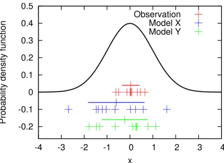
Figure 1 gives an illustration for the comparison of two 10 year model data sets (blue and green) and a 10 year observational data set (red). All are produced with computer generated random numbers for Gaussian distribution (black line) with expectation 0 and standard deviation 1. Note that this example neglects any uncertainties in the 20

observational data, i.e.σ_obsunc=0 and just takes into account an interannual variability.

In this example the underlying probability distribution is identical for the “model” and “observational” data. Hence model and the reality are identical, implying that the model is representing the reality perfectly. However, the 10 realisations for either “model run”

and the “observations” differ.

25

(6)

ACPD

9, 14141–14164, 2009

metrics”

Title Page

Tables Figures

◭ ◮

Back Close

Full Screen / Esc

the uncertainty of the grade. Then the estimates for the probability distributions have to be compared and a decision can be made whether the model represents the reality or not. Note that in the example the assumed distribution is Gaussian, the estimates

for the expectation (which is 0 in the example) is the sample mean value (differing from

zero) and for the standard deviation the sample standard deviation of the data. 5

2.2 When is a model better than another?

Model grades are used and will be used to rank models. Grades condense a complex context into a single number. However, as shown in Fig. 1, every intercomparison can only lead to a grade within a certain error range, which depends on a large number of

parameters. Hence two models (Fig. 1) might get two very different grades, however

10

with errorbars that are that large that the grades themselves do not differ statistically.

Therefore a grade itself is meaningless, unless an estimate for the uncertainty is given. Two model results are given (blue and green) in the example above (Fig. 1). They are

realisations (random samples) of the same random variable (X), which in this case has

a normal distribution with expectationE(X)₌0 and standard deviationS(X)₌1 (N(0,1)).

15

However, their gradings differ: Model X has a grade of 0.77 and Model Y of 0.46, when

applying formula (4) of WE08:

g= (

1−_n1

g

|µmodel−µobs|

σ_obs ,if 1 n_g

|µmodel−µobs|

σ_obs ≤1

0, else (1)

whereµmodelandµobs are the sample mean values of the model sample and

observa-tional sample, respectively. σobs is the sample standard deviation of the observational

20

data andn_g a factor (here: 3 as in WE08), which relates the difference of sample mean

values of the observations and model data tong times the sample standard deviation

of the observational data.

(7)

ACPD

9, 14141–14164, 2009

metrics”

Title Page

Tables Figures

◭ ◮

Back Close

Full Screen / Esc

In the following, terms and definitions are given. These form the basis for a systematic analysis, which is performed to show that the example, given above, is not an extreme outlier, but a representative example. The methodology can also be used as a basis for analysing further grading approaches.

3 Terms and definitions

5

In the following, X, Y, Z denote random variables representing a given diagnostic

for two models “Model X” and “Model Y” and observations. We are considering N

realisations of either Model X and Model Y, i.e. we have 2 samples, X1, ..., XN, and

Y1, ..., YN, and a sampleZ1, ..., ZM for the observations with sample sizeM.

We assume that the random variables have normal distributions, with expectations 10

E(X),E(Y) andE(Z) and standard deviationS(X), S(Y) and S(Z). To be consistent

with WE08, we denote the sample means ofX1, ..., XN, Y1, ..., YN, and Z1, ..., ZM as

µmodX, µmodY, and µobs. Note that in this case µ is not the expectation. In analogy,

the sample standard deviations are given byσ_modX,σ_modY, and σ_obs. Further, we

de-noteEr and Sr the real expectation and real standard deviation, describing the real

15

atmosphere. Hence a model is perfect ifE(X)=Er andS(X)=Sr and observations are

perfect ifE(Z)₌Er andS(Z)₌Sr.

FurtherGX andGY denote random variables of the grading of Model X and Model Y,

and GX1, ..., GXK and GY1, ..., GYK are samples of the grades of Model X and Y,

re-spectively. The samples have a sample sizeK each and are calculated on the basis of

20

samples of the random variablesX,Y andZ with sample sizesN for the models and

M for the observations. The sample mean values are given byµGX and µGY, i.e.µGX

and µ_GY are the mean values of K grades of either Model X and Y with N samples

of the random variablesX and Y (models) and M samples of the random variableZ

(observational data). Note that for one specific model run (as in WE08) the sample 25

sizeK equals 1. The expectations of the random variableGX andGY areE(GX) and

(8)

ACPD

9, 14141–14164, 2009

metrics”

Title Page

Tables Figures

◭ ◮

Back Close

Full Screen / Esc

A model is then statistically different from the observations, if the null hypothesis

H₀: “Model and observations have the same expectation” can be rejected and the

alternative hypothesis H1: “Model and observations are different” can be accepted.

For a model that does not differ statistically from observational data, i.e. forE(X)=E(Z)

andS(X)₌S(Z), we determine the threshold valuegobs(p) for which the probability that

5

G≤gobs(p) is p, i.e.P(G≤gobs(p))₌p, where pis the probability that H₀is erroneously

rejected. (We usep=1% and 5% in the following.) If the realisationGX1of the grading

of Model X is smaller thangobs(p), we reject the null hypothesis and regard the model

as statistically significantly di_fferent from the observations.

A model is then considered imperfect, if the null hypothesis H0: “Model and reality

10

have the same expectations” is rejected and the alternative hypothesis “Model and

reality have di_fferent expectations” is accepted. Hence we determine the threshold

valuegreal(p), whereP(G<greal(p))=p.

Note that these two tests seem to be very similar, however they have different

impli-cations. They di_ffer in the expectation and standard variation of the random variable

15

Z, which are E(Z) andS(Z) in the first case and Er and Sr in the second case. In

general, observational data are erroneous, which means that E(Z)6=Er orS(Z)6=Sr.

This has an impact on the grading, which we will describe in detail below.

Two model gradings are then statistically different, if the null hypothesis H0: “Grade

of Model X and grade of Model Y are equal” can be rejected and the alternative hypoth-20

esis H₁: “Grades of Model X and Model Y are different” can be accepted. Hence we

determine the threshold value∆g(p), whereP(|GX−GY|>∆g(p))=p, withE(X)=E(Y)

andS(X)=S(Y).

The statistical tests given in WE08 (their Sect. 2.2) are special cases

identi-cal to those described above, with the assumptions E(Z)=Er and S(Z)=Sr and

25

σmodX=σmodY=σobs. Our analysis will show that there is no disagreement between our

(9)

ACPD

9, 14141–14164, 2009

metrics”

Title Page

Tables Figures

◭ ◮

Back Close

Full Screen / Esc

results drastically.

4 Examples

4.1 A perfect model and perfect observations

Let us assume that we have a perfect model and that we know perfectly the regarded diagnostic of the reality. Further we assume that the values of the individual years 5

(here: N=M=10 years) have normal distributions. Since model and observations are

considered to be perfect in this case, the model’s and observational’s expectations and

standard deviations are equal:E(X)=E(Z)=Er=0 andS(X)=S(Z)=Sr=1.

What is the expectation of the grading E(G)? Is it simply: E(G)=1−1₃|E(X_S(Z))−E(Z)|=1?

No, becauseE(|X−Z|)6=|E(X)−E(Z)|. 10

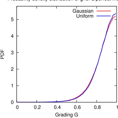
We estimate E(G) by means of a Monte Carlo simulation. We perform K=100 000

realisations of G. Each has random samples of X and Z with sample size N. The

resulting probability density function is given in Fig. 2. The derived sample mean value

for the grading isµG=0.87 (since K is large µG already converged to E(G)) and the

median is 0.88. They hence differ remarkably from 1. Calculating thep=5% (1%)

per-15

centile from the frequency distribution (Fig. 2) gives a value ofgobs(p)=greal(p)=0.65

(0.5) for this case.

For illustration purpose we additionally assume an uniform distribution of the random

variablesX andZ, with values between−1 and+1. The resulting pdf forGis the blue

line in Fig. 2. It only slightly differs from the Gaussian distribution.

20

4.2 A perfect model and imperfect observations

(10)

ACPD

9, 14141–14164, 2009

metrics”

Title Page

Tables Figures

◭ ◮

Back Close

Full Screen / Esc

derived. They also have some uncertainties related to the representativity (Lary and Aulov, 2008, e.g.).

Let us assume that (as above) the reality can be described by an expectation Er

and a standard deviation Sr. If we had perfect observations the sample mean value

µ_obs would be close toEr, for a large number of observational data (M). Let us now

5

assume that the observational data have an error. We express this error by an offset in

the expectation and standard deviation:E(Z)=Er+α×Sr andS(Z)=β×Sr. I.e. the

ob-servations have an error expressed by a multiple (or fraction) of the standard deviation, which is ithe interannual variability in the case of annual mean data.

An uncertainty in the expectation (=α) of 50% to a factor of 3 of the standard

de-10

viation is a reasonable assumption, as we will show in following by 2 examples. For

mid-latitude (35◦N–60◦N) total ozone columns, the interannual variability is in the range

of 5% and the differences between the various datasets (Ground-based, SBUV, NIWA,

GOME) are around 2–3%, which is around 50% of the interannual standard deviation (see WMO (2006) p. 3.11) . Lary and Aulov (2008) presented distributions of HCl mea-15

surements, e.g. for January at 450 K to 590 K isentropic levels and between 49 and

61◦N. Differences between 3 measurement systems are around 0.3 ppbv, whereas the

interannual variability for HALOE January values is in the order of 0.1 ppbv, which gives

a factor ofα=3.

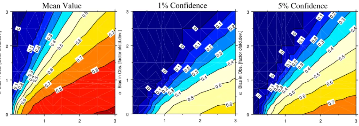
Figure 3 shows the mean values, 5% and 1% percentiles of the grading parameter. 20

The coordinate (0,1) represents the perfect observation, i.e., the example in Sect. 4.1. Clearly, the grading of the perfect model depends on the quality of the observational data. An increasing error in the expectation and hence the sample mean value leads to a reduction of the grading value. If the standard deviation in the observational data is lower than in reality, the grading value for the perfect model is also reduced. Whereas 25

the model gets a better grading, if the standard deviation of the observation is larger than in reality. The 5% and 1% percentiles (Fig. 3, mid and bottom) are decreasing to grading values of lower than 0.2, if either parameter has a 50% uncertainty.

(11)

ACPD

9, 14141–14164, 2009

metrics”

Title Page

Tables Figures

◭ ◮

Back Close

Full Screen / Esc

more than 0.1 have to be regarded to be perfect, for most of the observational data qualities regarded in this example.

4.3 Two identical models

Here the difference of two model gradings is investigated, i.e. we answer the question

“Is Model X statistically different from Model Y?” (see also Sect. 3).

5

Let us first assume that we have perfect observations and two identical, but

im-perfect models, with expectation E(X)=E(Y)=Er+αmod×S

r

and standard deviation

S(X)=S(Y)=βmod×S r

. (Both models are perfect for αmod=0 and βmod=1.) The

ex-pectation of either model grading is identicalE(GX)₌E(GY) and the di_fference of both

is 0. 10

In the example in Sect. 4.2, the expectation and standard deviation of the observa-tions were overlaid with an error. Here, the same error approach is applied to the 2

models. The parametersαmod andβmod, are randomly chosen, but equal for the

mod-els. They cover a deviation of maximum 2 timesSr. The parameter range is smaller

than in the previous example and actually describes small values for current CCMs. For 15

each of the 2 parameters 23 parameter settings were chosen in the given range. For

each setting 10 000 iterations (=K) were calculated to estimate the probability density

function of the di_fference in the two model gradesGX and GY, which add up to more

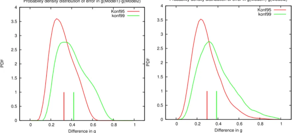
than 5 million iterations. Figure 1 shows one such an iteration, withN=M=10 values

for the observations, and Model X and Y, each. The frequency distribution of the 1% 20

and 5% percentiles for the absolute di_fference in the two model grades are shown in

Fig. 4. The mean 5% and 1% percentiles of the absoute difference for all regarded

parameter settings are 0.33 and 0.42 (vertical lines). However, in 5% of the parameter

settings 1% (5%) of the model differences are larger than 0.65 (0.51). And in 1% of the

parameter settings 1% (5%) of the differences are larger than 0.72 (0.55), defining the

25

1%- and 5%-percentiles.

In Fig. 4 (bottom) results are presented with inclusion of imperfect observational

data. The error is analogously considered: E(Z)=Er+αobs×S

r

and S(Z)=βobs×S

r

(12)

ACPD

9, 14141–14164, 2009

metrics”

Title Page

Tables Figures

◭ ◮

Back Close

Full Screen / Esc

αobs, σobs, αmod, βmod are independently chosen in the range [0.5,2]. The results are

similar to those with perfect observation, except that the confidence intervals are sig-nificantly increasing. The distributions have longer tails.

This leads to the conclusion that based on their gradings, two models are not

distin-guishable, unless the difference is larger than 0.71 and 0.86 for perfect and imperfect

5

observational data, respectively.

To summarize, these examples demonstrate that the statistical tests performed in WE08 are in agreement with our findings, however for special cases only. They give

a threshold g∗=0.7 for N=11, E(Z)=Er, S(Z)=Sr, and σobs=σmodX, which roughly

corresponds to our valuegreal(p=0.05)=0.65 for N=10,E(Z)=Er,S(Z)=Sr, however

10

σobs6=σmodX.

Further they give a threshold value of 0.3 for a statistically significant difference in

two model gradings at a 5% significance level, with the assumptionsN =11,E(Z)=Er,

S(Z)=Sr, andσobs=σmodX=σmodY. Our corresponding value is∆g

real

(p=0.05)=0.33 for

N₌10,E(Z)₌Er,S(Z)₌Sr, howeverσ_obs 6=σ_modX₌σ_modY.

15

The examples further show that the values for the special cases analysed in WE08 are misleading and that an adequate inclusion of observational errors change these thresholds drastically.

5 Consequences for the grading

In the last section we have investigated the reliability of the grading according to WE08. 20

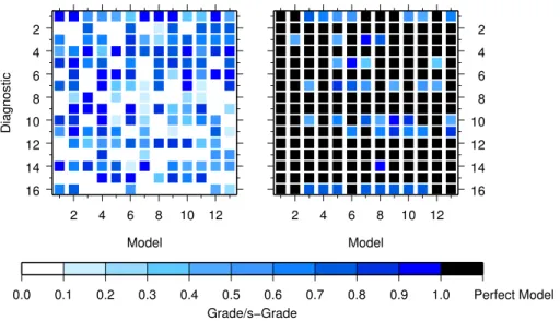
In this section we show its implications on the overall grading picture, i.e. on their Figs. 2 and 4. Applying the same procedure as in the previous sections, we randomly defined 16 diagnostics and 13 models. We then compare two grading approaches: the first is identical to that in WE08 and the second maps this grading to a 0 to 1 scale, where 1 is defined by the 5%-percentile of the grade from WE08. Any major quali-25

tative differences occurring between these gradings imply that the grading of WE08

(13)

expecta-ACPD

9, 14141–14164, 2009

metrics”

Title Page

Tables Figures

◭ ◮

Back Close

Full Screen / Esc

tion and standard deviation of the observations and models vary by randomly chosen

factorsα,β of maximum 2 and 3, respectively. Hence the models have potentially a

larger error than the observations. A detailed description of the parameters is given in the supplement material (see http://www.atmos-chem-phys-discuss.net/9/14141/2009/ acpd-9-14141-2009-supplement.pdf).

5

Figure 5 (left) shows the grading matrix in analogy to WE08, but for our random mod-els and observations. The diagnostic 1 and 4 has for all modmod-els high grades, whereas the diagnostic 13 and 16 leads to low grades for all models. For all of the diagnostics, we have calculated the 5% percentile for the expected grade of a perfect model and the given imperfect observations. Figure 5 (right) shows in black all grades, which do 10

not di_ffer significantly from reality. For all other grades the distance of the grade to the

confidence interval is taken as a deviation from the grade 1. Therefore, Fig. 5 (right) shows the significant model grades (s-grades), where a s-grade 1 indicates a model, which is not distinguishable from reality for the respective diagnostic. And all models

with a lower s-grade do differ significantly.

15

This changes the picture of the grading considerably. For diagnostic 1, which is char-acterised by high grades, the s-grades are high, but half of the models are imperfect. Whereas for diagnostic 2 many models have low grades, but since the confidence in-terval is large, all models are not distinguishable from reality and hence get a perfect s-grade of 1.

20

The quality of model 1 is similar to the other models with respect to the grade (Fig. 5, left). However, taking into account the confidence intervals for the grades, this model

becomes perfect with s-grades of 1 for all diagnostics. The qualitative difference in

the gradingg and statistical robust s-grade for our random models and observations

implies that the grades given in Fig. 2 in WE08 are not reliable. 25

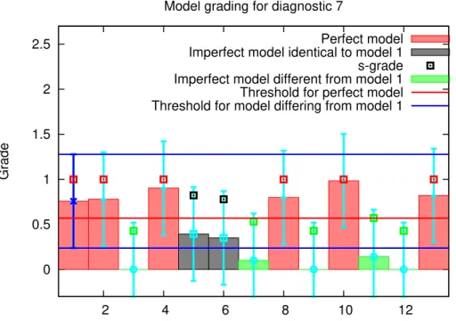
Figure 6 shows for the diagnostic 7 the grades of all models, comparable to Fig. 4 in WE08. We chose this diagnostic, because it is one of those showing a variability among the models in the grades and s-grades. We pick out model 1 and look for a

(14)

ACPD

9, 14141–14164, 2009

metrics”

Title Page

Tables Figures

◭ ◮

Back Close

Full Screen / Esc

reality and from model 1. Although model 5 and 6 (grey) are significantly different from

reality, they do not di_ffer significantly from model 1. Only the models 3, 7, 9, 11 (green)

differ significantly from model 1 and they also differ significantly from reality. Hence a

ranking of the models, which is suggested for a weighting of the multi-model mean is a

quite di_fficult task, e.g. although the s-grades di_ffer for model 1 and 5, both models do

5

not differ statistically significant from reality.

6 Conclusions

In the paper “Quantitative performance metrics for stratospheric-resolving chemistry-climate models” by Waugh and Eyring (2008) a method was introduced, which converts the outcome of a diagnostic, i.e. a comparison of climate-chemistry model data and 10

observational data, into a grade. A grading was applied to a number of diagnostics, leading to an overall model grade, which was proposed to be used as a weighting for a multi model mean.

In this comment, we focus on the statistical basis for the grading, with two aspects, the statistical confidence in the grade itself, and the possibility to statistically distinguish 15

two models with this grading. A summary is given in Table 1. Even if perfect observa-tions could be performed, and a perfect model is applied, an expected grading of 0.87 is obtained for a ten year dataset, the 99%-confidence interval for the model’s grade is

[0.5,1]. If we were not able to perform perfect observations, i.e. the observations have

a bias in the order of σ_obs, the interannual variability, then this confidence interval is

20

even enlarged to almost the whole range of the gradeg[0.01,1].

Two models differ statistically, if their grades differ by more than 0.33 and 0.42 for

an assumed error of 5% and 1%. However, these are mean values for a range of possible imperfect observational data. In 1% of the regarded errors in observational

data, a difference in the grade of more than 0.86 is needed to significantly distinguish

25

two models. And note that no answer is yet given on how much the models differ.

(15)

ACPD

9, 14141–14164, 2009

metrics”

Title Page

Tables Figures

◭ ◮

Back Close

Full Screen / Esc

the difference of two models, then this requires confidence intervals for each chosen

minimum di_fference. Hence a ranking of the models is hardly possible, and applicability

for a multi-model mean is very limited.

In Fig. 2 in WE08 the grades of a number of models and diagnostics are presented. The grading does not include any uncertainty in the observational dataset for most per-5

formance metrics. The parameterσobs in their formula describes either an interannual

variability or an uncertainty due to measurements. In the first case the measurements are implicitely regarded as perfect. And hence those are comparable to the example in Sect. 4.1. This implies that all models with a grade larger than 0.5 have to be regarded

to be perfect. Lower model grades indicate a significant difference to the observational

10

data. This is a qualitative statement and a further quantification on a statistically ro-bust basis cannot be given. However, the observational data have uncertainties, which should be accounted for. A thorough re-analysis of the grading would imply an esti-mate of the observational errors and inter annual variabilities of all used observational datasets, which has not been performed. If only a 25% or 50% uncertainty with respect 15

to the standard deviation is taken into account for the mean value and the standard de-viation, then the results for the random models presented here suggests that basically

none of the models presented in Fig. 2 in WE08 differ on a statistical basis.

The statistical tests, which we performed are in agreement with those performed in WE08. Their tests are however only special cases, which assume perfect observations 20

and that the interannual variability in the observational data equals the interannual vari-ability in the model data. The generalisation of the statistical test with the inclusion of

observational errors and differing interannual variability in the observational and model

data clearly shows a distinct difference in the results, e.g. grading confidence levels.

Moreover the inclusion of the statistical findings into the grading approach was not per-25

formed in WE08, which limits the interpretation of the results, since it is not clear, which

gradings are statistical significant or which model gradings differ statistically from each

(16)

ACPD

9, 14141–14164, 2009

metrics”

Title Page

Tables Figures

◭ ◮

Back Close

Full Screen / Esc

on the observational dataset.

A further challenge, which has not been addressed so far, is the robustness of a multi-diagnostic grade. In this comment, the grading properties were investigated on the basis of one diagnostic, only. If more than one diagnostic is taken into account, the variability of the individual grades has to be combined somehow with the confidence 5

intervals to provide an overall model grade with an uncertainty range.

The evaluation of models is an important part of model development. Multi-model approaches are the only way to address questions, which are of high importance to

politics and society. Model grading helps to better understand model differences and

determine specific model shortcomings. Hence a statistical robust grading is absolutely 10

necessary. We propose a detailed verification of any further grading methodology, e.g., on the basis of Monte Carlo simulations. And we further strongly suggest not to consider a grading approach in the way it was done for any further multi-modelling study. In detail, we propose for any future grading (a) to either calculate, estimate, or rely on expert judgement for all of the errors 1–3 described in 2.1, as well as for 15

the inter annual variability; (b) to include these uncertainties in the grading approach such that if the model data cannot be statistically distinguished from reality then and only then the grade is 1; (c) to also include these uncertainties in the determination of

grades lower than 1 (e.g. 1−x), such that for a given significance level, model data and

reality differ significantly by at least a certain value, which corresponds to some value

20

xin the grading.

Acknowledgement. We like to thank Darryn Waugh for a first discussion of this comment, which was very helpful for us in trying to understand the different views on a “grading”.

References

Lary, D. J. and Aulov, O.: Space-based measurements of HCl: Intercomparison and historical

25

(17)

ACPD

9, 14141–14164, 2009

metrics”

Title Page

Tables Figures

◭ ◮

Back Close

Full Screen / Esc

Waugh, D. W. and Eyring, V.: Quantitative performance metrics for stratospheric-resolving chemistry-climate models, Atmos. Chem. Phys., 8, 5699–5713, 2008,

http://www.atmos-chem-phys.net/8/5699/2008/.

World Meteorological Organisation (WMO): Scientfic Assessment of Ozone Depletion, Geneva, 2006.

(18)

ACPD

9, 14141–14164, 2009

metrics”

Title Page

Tables Figures

◭ ◮

Back Close

Full Screen / Esc

Interactive Discussion Table 1. Overview on the results from the Monte Carlo simulations. Imperfect observations

are defined by an o_ffset in the expectation and a multiple in the standard deviation (Details see text).

Percentile

5% 1%

(19)

ACPD

9, 14141–14164, 2009

metrics”

Title Page

Tables Figures

◭ ◮

Back Close

Full Screen / Esc

Interactive Discussion -0.2

-0.1 0 0.1 0.2 0.3 0.4 0.5

-4 -3 -2 -1 0 1 2 3 4

Probability density function

x

Observation Model X Model Y

(20)

ACPD

9, 14141–14164, 2009

metrics”

Title Page

Tables Figures

◭ ◮

Back Close

Full Screen / Esc

Interactive Discussion 0

1 2 3 4 5

0 0.2 0.4 0.6 0.8 1

PDF

Grading G

Probability density distribution of g for a perfect model

Gaussian Uniform

(21)

ACPD

9, 14141–14164, 2009

metrics”

Title Page Abstract Introduction Conclusions References Tables Figures ◭ ◮ ◭ ◮ Back Close

Full Screen / Esc

Printer-friendly Version Interactive Discussion 0 0.1 0.1 0.2 0.2 0.3 0.3 0.4 0.4 0.5 0.5 0.5 0.6 0.6 0.6 0.7 0.7 0.7 0.8 0.8 0 1 2 3 α

Bias in Obs. [factor ofstd.dev.]

1 2 3

β Obs.error in std.dev [factor of std.dev] Mean Value 0 0 0 0 0.1 0.1 0.1 0.1 0.2 0.2 0.2 0.2 0.3 0.3 0.3 0.4 0.4 0.4 0.5 0.5 0.6 0 1 2 3 α

1 2 3

β Obs.error in std.dev [factor of std.dev] 1% Confidence 0 0 0 0 0.1 0.1 0.1 0.1 0.2 0.2 0.2 0.2 0.3 0.3 0.3 0.3 0.4 0.4 0.4 0.4 0.5 0.5 0.5 0.6 0.6 0.7 0 1 2 3 α

1 2 3

β Obs.error in std.dev [factor of std.dev] 5% Confidence

(22)

ACPD

9, 14141–14164, 2009

metrics”

Title Page

Tables Figures

◭ ◮

Back Close

Full Screen / Esc

0 0.5 1 1.5 2 2.5 3 3.5 4

0 0.2 0.4 0.6 0.8 1

PDF

Difference in g

Probability density distribution of error in g(Model1)-g(Model2)

Konf95 konf99

0 0.5 1 1.5 2 2.5 3 3.5 4

0 0.2 0.4 0.6 0.8 1

PDF

Difference in g

Probability density distribution of error in g(Model1)-g(Model2)

Konf95 konf99

(23)

ACPD

9, 14141–14164, 2009

metrics”

Title Page

Tables Figures

◭ ◮

Back Close

Full Screen / Esc

2

4

6

8

10

12

14

16

Diagnostic

2 4 6 8 10 12

Model

2

4

6

8

10

12

14

16

2 4 6 8 10 12

Model

0.0 0.1 0.2 0.3 0.4 0.5 0.6 0.7 0.8 0.9 1.0 Perfect Model

Grade/s−Grade

(24)

ACPD

9, 14141–14164, 2009

metrics”

Title Page

Tables Figures

◭ ◮

Back Close

Full Screen / Esc

0 0.5 1 1.5 2 2.5

2 4 6 8 10 12

Grade

Model grading for diagnostic 7

Perfect model Imperfect model identical to model 1 s-grade Imperfect model different from model 1 Threshold for perfect model Threshold for model differing from model 1