Study of the electromyographic signal dynamic behavior in Amyotrophic Lateral Sclerosis (ALS)

(1)

Maria Marta Oliveira Antunes dos Santos

Licenciatura em Engenharia Biomédica

Study of the electromyographic signal dynamic

behavior in Amyotrophic Lateral Sclerosis (ALS)

Dissertação para obtenção do Grau de Mestre em Engenharia Biomédica

Orientadora : Carla Quintão, Professora Auxiliar, Faculdade de Ciên-cias e Tecnologia da Universidade Nova de Lisboa

Co-orientador : Hugo Gamboa, Professor Auxiliar, Faculdade de Ciên-cias e Tecnologia da Universidade Nova de Lisboa

Júri:

Presidente: Doutor Mário Forjaz Secca

Arguente: Doutor Alexandre Freire de Andrade

(2)

(3)

iii

Study of the electromyographic signal dynamic behavior in Amyotrophic Lat-eral Sclerosis (ALS)

Copyright c Maria Marta Oliveira Antunes dos Santos, Faculdade de Ciências e Tec-nologia, Universidade Nova de Lisboa

(4)

(5)

(6)

(7)

Acknowledgements

First I thank my supervisor, Professor Carla Quintão, for her guidance and patience, her vigorous spirit and knowledge. I am very grateful for her availability, ideas, motivation and encouragement. I thank my co-supervisor, Professor Hugo Gamboa, who offered me new ideas and solutions. I thank Doctor Professor Mamede de Carvalho and Doctor Su-sana Pinto for their collaboration, making possible to perform acquisitions from patients at Hospital Sta. Maria. I thank Ricardo Gomes for his patience and ideas, and all the staff ofPLUX – Wireless Biosignals, S. A., for receiving me every day.

A very big thank you to Luísa Gomes, for her help, patience and opinions; for the ev-eryday conversations we shared; these years would not have been the same without her. To Inês Vale, Inês Silva, David Branha and Catarina Cavaco I thank for these wonder-ful years; their friendship, support and motivation are essential. I also thank my oldest friends, who in spite of sometimes are away, are always in my heart.

(8)

(9)

Abstract

Amyotrophic Lateral Sclerosis (ALS) is a neurodegenerative disease characterized by motor neurons degeneration, which reduces muscular force, being very difficult to diag-nose. Mathematical methods are used in order to analyze the surface electromiographic signal’s dynamic behavior (Fractal Dimension (FD) and Multiscale Entropy (MSE)), eval-uate different muscle group’s synchronization (Coherence and Phase Locking Factor (PLF)) and to evaluate the signal’s complexity (Lempel-Ziv (LZ) techniques and Detrended Fluc-tuation Analysis (DFA)). Surface electromiographic signal acquisitions were performed in upper limb muscles, being the analysis executed for instants of contraction for ipsilat-eral acquisitions for patients and control groups. Results from LZ, DFA and MSE anal-ysis present capability to distinguish between the patient group and the control group, whereas coherence, PLF and FD algorithms present results very similar for both groups. LZ, DFA and MSE algorithms appear then to be a good measure of corticospinal path-ways integrity. A classification algorithm was applied to the results in combination with extracted features from the surface electromiographic signal, with an accuracy percentage higher than 70% for 118 combinations for at least one classifier. The classification results demonstrate capability to distinguish members between patients and control groups. These results can demonstrate a major importance in the disease diagnose, once surface electromyography (sEMG) may be used as an auxiliary diagnose method.

(10)

(11)

Resumo

A Esclerose Lateral Amiotrófica (ELA) é uma doença neurodegenerativa caracteri-zada pela degeneração progressiva de neurónios motores, o que reduz a força muscular, sendo muito difícil de ser diagnosticada. São usados métodos matemáticos de forma a caracterizar o sinal eletromiográfico de superfície (sEMG) de pacientes com ELA, com o objetivo de analisar o comportamento dinâmico do sinal (Dimensão Fractal (DF) e Multis-cale Entropy (MSE)), avaliar a sincronização de diferentes grupos musculares (Coerência e Phase Locking Factor (PLF)) e avaliar a complexidade do sinal (técnicas de Lempel-Ziv (LZ) e Detrended Fluctuation Analysis (DFA)). A aquisição de sEMG foi feita em mús-culos dos membros superiores, sendo a análise feita para momentos de contração para aquisições ipsilaterais tanto para o grupo de pacientes como para o grupo de controlo. Os resultados das análises de LZ, DFA e MSE apresentam capacidade de distinção entre o grupo de pacientes e o grupo de controlo, enquanto que os algoritmos de coerência, PLF e DF apresentam resultados muito similares para ambos os grupos. Os algoritmos de LZ, DFA e MSE aparentam, então, ser bons indicadores da integridade de percursos cor-ticoespinhais. Um algoritmo de classificação foi também aplicado aos resultados destes algoritmos em conjunto comfeaturesextraídas do sinal de sEMG, com uma percentagem de acerto de 70% para 118 combinações para pelo menos um classificador. Os resulta-dos da classificação demonstram capacidade de distinção entre os grupos de pacientes e controlo. Estes resultados podem demonstrar-se importantes no diagnóstico da doença, sendo que se poderá passar a usar electromiografia de superfície como método auxiliar de diagnóstico.

(12)

(13)

List of Figures

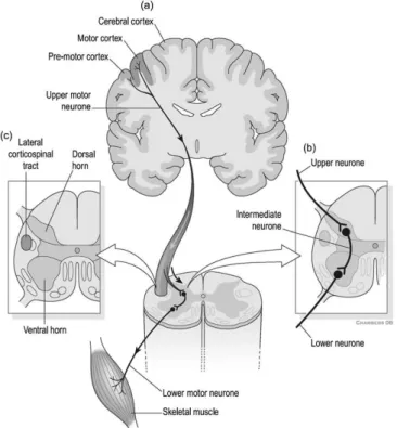
2.1 Lateral cortical spinal tract. (a) Descending motor pathways carry infor-mation from the brain to the spinal cord. (b) Region where Upper Motor Neuron (UMN)s interdigitate with Lower Motor Neuron (LMN)s. LMNs carry the information from UMNs to the muscles. (c) Location of the lateral cortical spinal tract in the spinal cord [1]. . . 9

2.2 Motor Unit: a Motor Neuron with several branches, each one of them terminating at different muscle fibers of the same type. This terminal branches are typically in a ‘One-To-One’ relationship with the muscle fibers (a muscle fiber receives only a terminal branch, and a terminal branch in-nervates only a muscle fiber) [2, 3, 4].. . . 10

2.3 Response to a single stimulus as a result of a single twitch contraction, which may last 25-75 ms [2]. . . 10

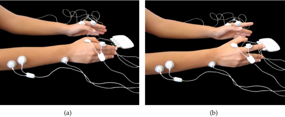
3.1 Simultaneous contralateral and ipsilateral experimental setup: Bioplux re-search device, placement of four EMG sensors and ground. (a) Instant of relaxation. (b) Instant of contraction. . . 22

4.1 Schematic representation of only 4 seconds of the 297 seconds (correspond-ing to 49 contractions) signal defined by eq. 4.2, withAdefined as1and

f placed at 15 Hz (a) Signal withφ(t)defined as Uniform noise. (b) Signal withφ(t)defined asπ/3 +t×0.1 . . . 30

4.2 Schematic representation of the signal defined by eq. 4.3 with 297 seconds (corresponding to 49 contractions) withAdefined as1andf placed at 30 Hz 30

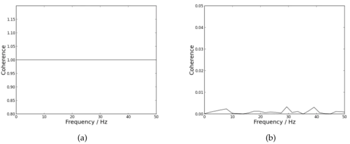
5.1 Coherence dependency on frequency for signals defined by eq. 4.3 withf

(16)

xvi LIST OF FIGURES

5.2 Coherence dependency on frequency, using NFFT placed as 512. (a) sults for coherence calculated between a random signal and itself. (b) Re-sults for coherence calculated between two random signals. . . 34

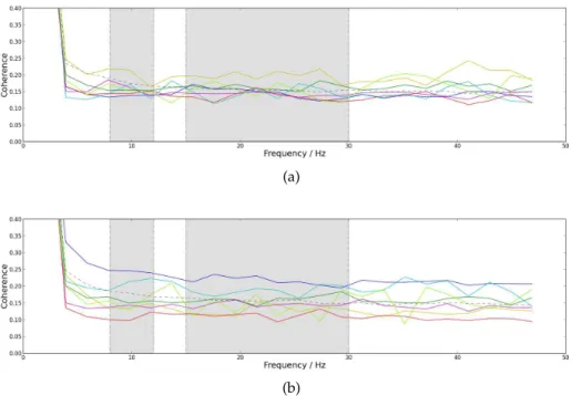
5.3 Mean coherence dependency on frequency with NFFT placed as 512. Straight line for patients and dashed line for controls. The first grey box delimitates the frequencies corresponding to the alpha band (8 −12 Hz). The sec-ond grey box delimitates the frequencies correspsec-onding to the beta band (15−30Hz). (a) Results from the left arm. (b) Results from the right arm. 34

5.4 Mean coherence dependency on frequency with NFFT placed as 512. The dashed line represents the group of control and the straight lines repre-sent the group of patients: yellow line is for onset form axial, dark blue line for Bulbar (B), red line for Left Lower Limb (LLL), dark green line for Left Upper Limb (LUL), light blue line for Primary Lateral Sclerosis (PLS), magenta line for Right Lower Limb (RLL) and light green line for Upper Limbs (UL). The first grey box delimitates the frequencies corresponding to the alpha band (8−12 Hz). The second grey box delimitates the fre-quencies corresponding to the beta band (15−30Hz). (a) Results for the left arm. (b) Results for the right arm. . . 35

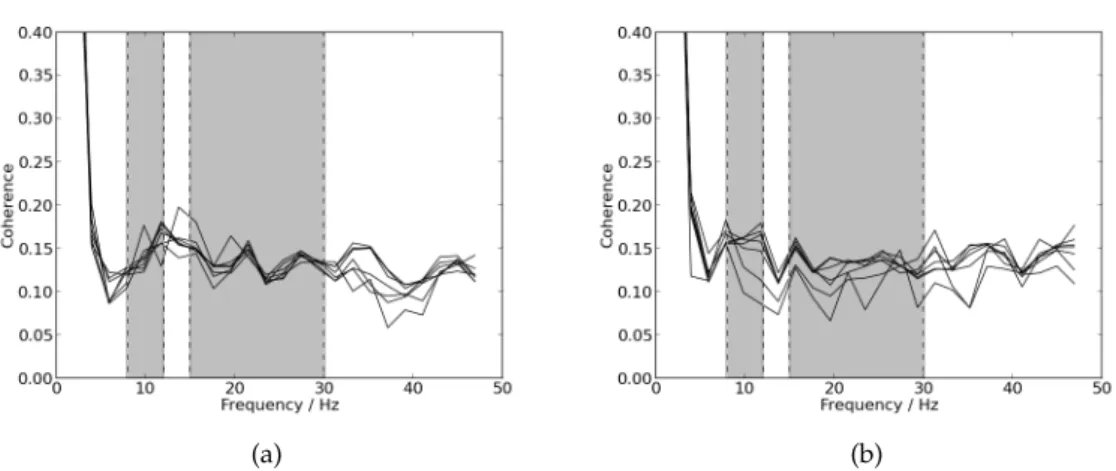
5.5 Coherence values dependency on frequency for the right arm for different lengths of the same signal. The first grey box delimitates the frequencies corresponding to the alpha band (8 −12 Hz). The second grey box de-limitates the frequencies corresponding to the beta band (15−30Hz). (a) Results for one member of the patients group. (b) Results for one member of the control group. . . 36

5.6 Coherence values dependency on frequency for the right arm for ten differ-ent contractions of the same signal starting with the first ten until the last ten. The first grey box delimitates the frequencies corresponding to the alpha band (8−12 Hz). The second grey box delimitates the frequencies corresponding to the beta band (15−30Hz). (a) Results for one member of the patients group. (b) Results for one member of the control group. . . 36

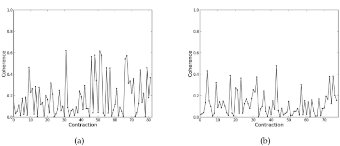
5.7 Coherence values for each contraction for the right arm for frequency 17.58 Hz. (a) Results for one member of the patients group. (b) Results for one member of the control group. . . 37

(17)

LIST OF FIGURES xvii

5.9 Maximum coherence values dependent on frequency for each member of patients and control groups for the right arm, with NFFT placed at 512. The grey boxes delimitates different frequency bands (from left to right, 15 – 22 Hz, 28 – 36 Hz and 38 – 43 Hz), being all the other frequencies represented by the white boxes. (a) Results for the group of patients. (b) Results for the group of control. . . 38 5.10 Mean coherence values dependency on frequency for the right arm, with

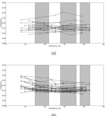
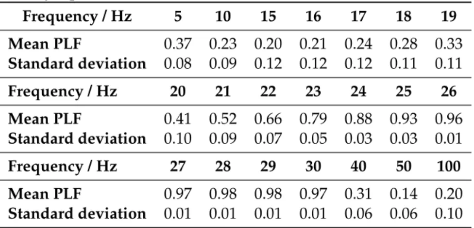
NFFT placed at 4096. The used signals are a concatenation of all the con-tractions existent in each signal. The straight red line represents the pa-tients group and the straight green line represents the control group. The first grey box delimitates the frequencies corresponding to the alpha band (8−12Hz). The second grey box delimitates the frequencies corresponding to the beta band (15−30Hz). . . 38 5.11 Phase Locking Factor (PLF) mean values dependency on frequency for

pa-tients by the straight line and for controls by the dashed line. The first grey box delimitates the frequencies corresponding to the alpha band (8−12 Hz). The second grey box delimitates the frequencies corresponding to the beta band (15−30Hz). (a) Results from the left arm. (b) Results from the right arm.. . . 39 5.12 PLF value for the right arm of the member of patients group calculated 500

times for one lagged contraction (time lag of 250 points to the left and 250 points to the right). A time lag of 500 points corresponds to 0.5 s. The blue vertical line indicates the maximum value of PLF. (a) Results for 17 Hz (PLF is 0.444 for point 34). (b) Results for 29 Hz (PLF is 0.448 for point -150). 40 5.13 PLF value for the right arm of the member of control group calculated 500

times for one lagged contraction (time lag of 250 points to the left and 250 points to the right). A time lag of 500 points corresponds to 0.5. The blue vertical line indicates the maximum value of PLF. (a) Results for 17 Hz (PLF is 0.409 for point 249). (b) Results for 29 Hz (PLF is 0.512 for point -9). 41 5.14 PLF value for the right arm calculated 200 times for the central 500 points

window of one lagged contraction (time lag of 100 points to the left and 100 points to the right). A time lag of 200 points corresponds to 0.2 s. The blue vertical line indicates the maximum value of PLF. (a) Results for 17 Hz for the member of the patient group (PLF is 0.956 for point 16). (b) Results for 17 Hz for the member of the control group (PLF is 0.493 for point -8). . . . 41 5.15 PLF value for the right arm for one contraction divided in 5 windows of

(18)

xviii LIST OF FIGURES

5.16 Average of the base 10 logarithm ofL(k)plotted againstkfor both groups.

The red straight lines correspond to the linear regressions for the patients group. The green straight lines correspond to the linear regressions for the control group. (a) Left hand; the curve fitting is described by−1.98x+ 4.00 for the patient group and by−1.98x+ 4.21for the control group (b) Left forearm; the curve fitting is described by −1.98x + 3.94 for the patient group and by−1.98x+ 3.99for the control group (c) Right hand; the curve fitting is described by−1.99x+ 3.91for the patient group and by−1.98x+ 4.21for the control group (d) Right forearm; the curve fitting is described by−1.98x+ 3.93for the patient group and by−1.98x+ 4.04for the control group.. . . 42

5.17 Base 10 logarithm ofF(n)plotted againstnfor (a) White noise for a signal with 300000 ms (α = 0,502); (b) Pink noise for a signal with 297000 ms (α= 0,974); (c) Brownian noise for a signal with 300000 (α= 1,499). . . . 45

5.18 Base 10 logarithm ofF(n)plotted against naveraged among all subjects within each group. The black dashed line corresponds to the patient group and the black straight line corresponds to the control group. The red straight lines correspond to the linear regressions of each segment for the patients group. The green straight lines correspond to the linear regressions of each segment for the control group. The curve fitting for each segment is shown in the graph. (a) Results for the left hand. (b) Results for the left forearm. (c) Results for the right hand. (d) Results for the right forearm. . . 46

5.19 Schematic representation of the Sample Entropy value for each scale (each

τ) for a signal with length 80 s. The used tolerance isr= 0.15σ. (a) Results for White noise. (b) Results for Pink noise. . . 47

5.20 Sample Entropy mean value for each scale obtained for tolerance, τ, of

0.15σ. The straight line represents the patient group, and the dashed line represents the control group. (a) Results for the left hand. (b) Results for the left forearm. (c) Results for the right hand. (d) Results for the right forearm. . . 48

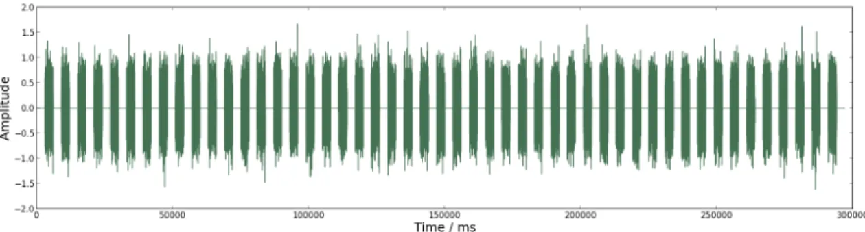
5.21 Signal from the right hand acquired from a healthy subject (moment of contraction with 179150 ms).. . . 49

(19)

LIST OF FIGURES xix

5.23 PLF values dependency on frequency for one long contraction of a healthy subject. The first grey box delimitates the frequencies corresponding to the alpha band (8−12Hz). The second grey box delimitates the frequencies corresponding to the beta band (15−30Hz).(a) Results from the left arm. (b) Results from the right arm.. . . 50 5.24 Sample Entropy value for each scale for one long contraction of a healthy

subject for tolerance,τ, of0.15σ. (a) Results for the left hand. (b) Results

for the left forearm. (c) Results for the right hand. (d) Results for the right forearm. . . 51

A.1 Mean coherence values dependency on frequency (straight line) and stan-dard deviation (dotted red line) for the patients group. The first grey box delimitates the frequencies corresponding to the alpha band (8−12 Hz). The second grey box delimitates the frequencies corresponding to the beta band (15−30Hz). (a) Results from the left arm. (b) Results from the right arm. . . 65 A.2 Mean coherence values dependency on frequency (straight line) and

stan-dard deviation (dotted red line) for the control group. The first grey box delimitates the frequencies corresponding to the alpha band (8−12 Hz). The second grey box delimitates the frequencies corresponding to the beta band (15−30Hz). (a) Results from the left arm. (b) Results from the right arm. . . 66 A.3 Mean PLF values dependency on frequency (straight line) and standard

deviation (dotted line) for the patients group. The first grey box delimitates the frequencies corresponding to the alpha band (8−12Hz). The second grey box delimitates the frequencies corresponding to the beta band (15−

30Hz). (a) Results from the left arm. (b) Results from the right arm. . . 66 A.4 Mean PLF values dependency on frequency (straight line) and standard

deviation (dotted line) for the control group. The first grey box delimitates the frequencies corresponding to the alpha band (8−12Hz). The second grey box delimitates the frequencies corresponding to the beta band (15−

(20)

(21)

List of Tables

5.1 Representation of the PLF mean and standard deviation values for the syn-thetic signals defined by eq. 4.2 withA= 1,t= 297sandf = 15Hz.. . . . 39 5.2 Mean and standard deviation values of Fractal Dimension (FD) coefficient

for patients and control group. . . 43 5.3 MFL values for patients and control group. . . 43 5.4 Lempel-Ziv (LZ) coefficient for a binary sequence obtained from the

fil-tered used signal with threshold defined as 0. . . 44 5.5 LZ coefficient for a binary sequence obtained from the rectified filtered

used signal with threshold defined as 0.4. . . 44 5.6 LZ coefficient for a binary sequence obtained from the envelope of the

rec-tified filtered used signal with threshold defined as 0.12. . . 44 5.7 DFAα1coefficient mean and standard deviation values for both groups. . 47 5.8 DFAα2coefficient mean and standard deviation values for both groups. . 47 5.9 Multiscale Entropy (MSE) mean and standard deviation values, for both

patients and control groups. . . 48 5.10 Detrended Fluctuation Analysis (DFA) coefficients values, α1 andα2, for

one control for one long contraction of a healthy subject with 179150 ms. . 51 5.11 Classification results for the right arm for Decision Tree, Random Forest

and AdaBoost Classifiers. . . 52

B.1 Classification results for the right arm for Nearest Neighbors and Decision Tree Classifiers. . . 70 B.2 Classification results for the right arm for Random Forest and AdaBoost

(22)

(23)

Acronyms

ALS Amyotrophic Lateral Sclerosis

AP Action Potential

B Bulbar

CNS Central Nervous System

DC Direct Current Component

DFA Detrended Fluctuation Analysis

ECG Electrocardiogram

EEG Electroencephalogram

EMG Electromyography

FD Fractal Dimension

FFT Fast Fourier Transform

FPs Fasciculation Potentials

IDFT Discrete Inverse Fourier Transform

LLL Left Lower Limb

LMN Lower Motor Neuron

LUL Left Upper Limb

LZ Lempel-Ziv

MFL Maximum Fractal Length

(24)

xxiv LIST OF TABLES

MR Magnetic Resonance

MSE Multiscale Entropy

MU Motor Unit

MUAP Motor Unit Action Potential

MUNE Motor Unit Number Estimation

MUPs Motor Unit Potentials

NCS Nerve Conduction Studies

NFFT Nonequispaced Fast Fourier Transform

PLF Phase Locking Factor

PLS Primary Lateral Sclerosis

RLL Right Lower Limb

RMS Root Mean Square

RUL Right Upper Limb

sEMG Surface Electromyography

UL Upper Limbs

(25)

1

Introduction

1.1 Motivation

Amyotrophic Lateral Sclerosis (ALS) is a neurodegenerative disease which is character-ized by motor neurons progressive degeneration [5, 6,7]. This is a fatal and very pro-gressive disease, which is responsible for abnormal motor activity [5,6,7,8,9]. However, neurodegeneration is believed to begin long before the development of any symptoms [10]. Therefore, ALS is very difficult to diagnose and to control. On top of that, there aren’t any available curative treatments for this disease, as well as a reliable biomarker of disease activity and progression [6,9].

This disease incidence, which affects people throughout the world, is not exactly known [9]. Population studies including European citizens have demonstrated an uni-form incidence of 2.16 per 100000 person-years, with slightly higher incidence among men than women [6,9]. More recent studies established an approximately1.5per100000

worldwide incidence [7].

(26)

1. INTRODUCTION 1.2. Objectives

1.2 Objectives

The purpose of this thesis is to study the electrical activity of different muscle groups both inALSpatients and in a control group.

Surface electrodes will be used to acquire a surface electromyographic (sEMG) signal from both groups, which will be processed and analyzed. Physiological features will be extracted and variations in the electric signal between both groups will be studied.

The algorithms used to process the signal include:

• Coherence analysis to analyze frequency correlations between different muscle groups;

• Phase Locking Factor calculations to detect synchronization between different mus-cle groups;

• Fractal Dimension and Multiscale Entropy to evaluate the signal’s chaotic behavior;

• Lempel-Ziv and Detrended Fluctuation Analysis methods to estimate the signal’s complexity.

There will also be applied classification algorithms in order to distinguish both groups. These algorithms are: k-Nearest Neighbor, Decision Tree, Random Forest, AdaBoost and Naïve Bayes.

Ultimately, the aim is to determine if an individual is affected by a neurodegenerative disorder, particularlyALS, evaluate the disorder stages of progression, as well as distin-guish between healthy individuals and individuals affected by this disease. Therefore, this project requires an acquisition protocol, signal recordings and signal processing.

1.3 State-of-the-art

(27)

1. INTRODUCTION 1.3. State-of-the-art

Babinski sign and hyperreflexia may be indicators of impairment in corticospinal track, they can’t alone reflect such damage [14].

Several techniques have been used in an effort to detect, evaluate and quantify motor degeneration inALS, as well as exclude other disorders with identical symptoms. These include Needle Electromyography (EMG), Nerve Conduction Studies (NCS), Motor Unit Number Estimation (MUNE), used mainly in the research setting, Neurophysiological In-dex, Transcranial Magnetic Stimulation and Neuroimaging techniques, such as Magnetic Resonance Spectroscopy and Diffusion Tensor Magnetic Resonance (MR) Tractography, among others. In addition to these techniques, Sniff Nasal Pressure and Maximum Vol-untary Isometric Contraction have also been investigated though they can’t be used as a test for all patients. Aside from these techniques, which can be used as disease progres-sion markers, disease modifying pharmacological therapies have been investigated as well, although the results remain elusive. However, at present time, Riluzole is the only pharmacological agent with modest effect, and its effects could be considerately better if administrated early in the disease course [5,7,9,11,14,15] .

Upper Motor Neuron integrity can be evaluated through the investigation of oscil-latory activity propagation. Rhythmic activity in the alpha (8 - 12 Hz) and beta (15–30 Hz) frequency bands can be recorded from the motor cortex and coherence may be com-puted. The results of this coherence analysis evidence synchronization between cortex and contralateralEMGin the beta band, which suggests that these oscillations are con-veyed from cortex to muscle. Therefore, it is believed that pyramidal tract neurons are related to generation and propagation of beta band oscillations [14]. Beta band coupling (in normal subjects) can be observed between different muscles as well – intermuscular coherence – [14, 16], which reveals the existence of a shared cortical drive. Moreover, coherence between muscles and the motor cortex is a measure of oscillatory coupling between electromyographic discharge and the central nervous system motor elements, whereas the phase difference provides an estimate of the temporal delay between cortex andEMG[17]. Also, during steady muscle contraction, it is observed maximum inter-muscular coherence. Interinter-muscular coherence appears to be dependent on supraspinal structures, since it disappears after impairment of these structures. However, it doesn’t appear to depend on anterior horn cells. Beta band and intermuscular coherence have also been proved to be greatly influenced by sensory afferents [14]. In fact, cortical coher-ence has been proved to involve transmission in both descending (motor) and ascending (sensory) direction [18]. Concerning the alpha band, it was stated byFarmer et al. that physiological tremor of approximately 10 Hz has been associated to Motor Unit (MU) synchrony at 8-12 Hz [19,16].

(28)

Coherence at frequencies from 1 Hz to 45 Hz (in adults) have been associated to Mo-tor Unit firing recorded from pairs of cocontracting muscles, being maximal in a low frequency range (1-12 Hz) and in a high frequency range (16-32 Hz, with maxima at ap-proximately 20 Hz). Moreover, cortical coherence at apap-proximately 20 Hz, as well as Motor Unit synchrony are concomitant with important common drive, which conducts to coactivation of closely related muscles [19]. Farmer et al.[19] have also suggested that increased speed and accuracy when performing a motor task and more efficient Motor Unit recruitment are associated with a 20 Hz coherence as well.

Either normal or pathological signals can be characterized by means of theFDstudy of an EMG signal. Small changes in the FD of these signals are indicators of muscle activation in a linear way. This muscle activation is related with voluntary contraction since it can be measured as a fraction of its maximum value. Flexion-extension speeds and load are linearly related with FDas well. MUrecruitment patterns complexity can also be quantified usingFD[20]. Arjunan et al. [21] confirmed these findings observing a relationship between muscle contraction complexity andFD. Therefore, changes in a muscle shape and contraction may influence this complexity, and consequently theFD as well. As a matter of fact, small changes of muscle contraction are concomitant with small variations ofFDwhile high level of muscle contraction or stretch presents a higher impact on this measure [20].Arjunan et al.[22] reached the conclusion that the strength of a muscle’s contraction is better estimated based on Maximum Fractal Length (MFL), even for very small muscle contraction strength, rather than FD(which is confirmed in [20] where it is proposed the use of the signal’s overall length as a measure of muscle activity) or other features such as Variance (VAR), Waveform Length (WL) and Root Mean Square (RMS). Accordingly,Arjunan et al. [21] also evidenced that the contraction’s strength of the associated muscles is related toMFL. These authors have applied fractal density and MFLto the identification of a set of finger-and-wrist flexion-based actions in conditions of very weak muscle activity. They validated this system and suggested it would be useful for a human computer interface or the control of a prosthetic hand [21].

(29)

LZcomplexity measure reflects variations in synchronization of firingMUs and in mus-cle fiber conduction velocity consistent with situations of fatigue, this feature is consid-ered to have higher performance when compared with median frequency, since median frequency is not reliable to what concerns to synchrony. These authors have also con-firmed these results with their previous work with multi-fractal Detrended Fluctuation Analysis (DFA). TheLZmeasure is a well suited feature regardingsEMGanalysis, par-ticularly during dynamic contractions (highly non-stationary signal), since this feature doesn’t make any assumption of stationarity (rather than other analysis techniques such as power spectrum estimations, among others) [23].

Phinyomark et al. [25] proposed the use ofDFA in order to studyEMGsignals, since they exhibit complex and nonlinear properties. They evidenced the efficacy of this method to discriminate upper-limb movements. These authors also showed that theDFAmethod outperforms other methods (e. g. the correlation dimension method and the Higuchi method), since it is a stable technique to quantify fractality and to establish self-similarity, being a robust method in the presence of nonstationarity time series and trends. TheDFA method is also a suitable tool regarding the characterization of short-time nonstationary EMGtime series. This method has also been used as a fatigue index in previous studies [25].

Entropy is a feature which can detect and quantify differences in theEMGsignal am-plitude distributions due to neuromuscular conditions (pathology) [26]. This feature has been successfully applied to physiological signals, in order to quantify their degree of complexity. Multiscale Entropy (MSE) has been proved to be more effective than Single-scale Entropy in this quantification, since it considers multiple spatiotemporal Single-scales [27,28]. Thuraisingham et al. [28] analyzed a deterministic chaotic system (the Lorentz equation) and evinced that theMSEsignature obtained from a time series is dependent of the sampling time interval, the oscillation’s period and the correlation time. For in-stance, sampling rate can affect MSE signature by causing decorrelation and suppress periodicities. Moreover, the time scales under consideration influence greatly the degree of complexity. So, if the sampling time is greater than the correlation time and the period of probable nonlinear frequencies, chaotic time series (with or without nonlinear frequen-cies) exhibit the sameMSEsignature as white noise (uncorrelated fluctuation) [28]. If the sampling time is smaller than the correlation time in the sampled data (or the correlation time is greater than periods of possible nonlinear frequencies), the Sample Entropy will firstly increase (because of decorrelation) and subsequently decrease according to the law of the averages.

(30)

1. INTRODUCTION 1.4. Thesis Overview

reliable algorithm it is necessary to apply a classification process and to compare differ-ent classifiers [29,30]. However, the analyzed features have great influence on the results [29]. Considering feature extraction, the size of the time window may also influence the results, being an important factor in the sampling parameters for EMG signal processing [30].

k-Nearest Neighbor is a relatively simple and fast algorithm, important characteris-tics in the classification process [30]. Decision Tree methods have also been used for deal-ing with classification problems in various domains, such as pattern recognition, data mining, web mining and signal processing, among others. However, standard Decision Tree algorithms can only handle discrete attributes [31]. The Decision Tree algorithm has usually good performance for large data sets in a short time [32]. Random Forest algo-rithm has been tested with real and simulated data sets. The results have been proven to be very accurate. This algorithm is fast, versatile and can be applied to very large data sets. It has also been shown its robustness against noise in the outcome compared with several other methods [33]. Discrimination between subject or patient group concerning age, gender and injuries in athletes has been proven to be effective using a classification approach with generic features and AdaBoost [29]. Naïve Bayes method has shown to be competitive among much sophisticated induction algorithms concerning experiments on real world data, despite the assumption of conditional independence [31].

1.4 Thesis Overview

(31)

2

Theoretical background

2.1 Scientific support

2.1.1 Amyotrophic Lateral Sclerosis (ALS)

ALS is a neurological and rapid progressive degenerative disease, also known as Lou Gehrig disease or Motor Neuron Disease (MND). This disorder is characterized by both Upper and Lower Motor Neurons degeneration, involving brainstem and also multiple spinal cord innervation regions. In fact, corticospinal tract integrity may be damaged in any region from layer V pyramidal neurons from the motor cortex, where UMN(also known as Betz cells) are located, to the anterior horn of the spinal cord, whereLMNare located [6,9,14]. Thus, this disorder is characterized according to the affected neurologi-cal regions: bulbar, cervineurologi-cal, thoracic and lumbrosacral [5,12,14]. Clinical manifestations of ALS are associated to each one of these regions, and the identification of different phenotypes has significant importance regarding patients’ prognosis and survival. Some adverse prognostic indicators include reduced time among first symptoms and disease presentation, low forced vital capacity and increased age of onset [5].

(32)

2. THEORETICAL BACKGROUND 2.1. Scientific support

sleep disturbances, among other indirect symptoms which are a repercussion of the di-rect ones. After the first symptoms, death may occur within 3 – 5 years for most of the patients [5,6,7,9] .

While 90% of cases ofALSare sporadic or idiopathic, approximately 10% ofALScases are familial [5,6,7, 9]. However, although several theories concerningALScauses and pathogenesis have been studied, this disease etiology still remains poorly understood [5,6,7]. FamilialALSis related most commonly with autosomal-dominant patterns, but also with X-linked and autosomal recessive patterns. More than 75 causative mutations of ALS have been described over the years, being a point mutation in the copper/zinc ion-binding superoxide dismutase (SOD1) the first one to be reported [5, 7, 9]. These mutations in SOD1 gene provoke a toxic gain of function of the SOD1 protein, instead of a reduction of activity of the same protein, as previously supposed. However, the most likely common mutation recently described is a hexanucleotide repeat expansion of the chromosome 9 open reading frame 72 (C9orf72) gene. These genes are not only associated withALSfamilial cases, but also with a reduce number of apparently sporadic cases [7,9]. ALS has also been linked with environmental and occupational risk factors, including heavy-metal toxic effects, neurotoxins military service, cigarette smoking, agricultural or factory work and physical exertion. Nevertheless, it wasn’t determined a definite causal relationship with any of these factors [5,6,7,9]. Other pathogenic hypothesis regarding this disorder are mitochondrial dysfunction, increased intracellular calcium, autophagy, sodium/potassium ion pump dysfunction, disrupted axon transport systems and pro-tein disaggregation. The latter is associated with mutations in the genes for fused in sar-coma (FUS) and TAR DNA binding protein-43 (TDP-43). Angiogenin (ANG, ribonucle-ase, RNase A family, 5) and optineurin (OPTN) are also associated to clinical phenotype. TDP-43, FUS and ANG are involved in RNA trafficking [7,9]. In addition to the previous hypothesis, glutamate-induced excitotoxicity can incite neurodegeneration. In literature [9] two theories are described for the beginning of this disorder, considering the mech-anism ofMUdegeneration mediated by glutamate-induced excitotoxicity. They are the “dying - forward” and the “dying - back” hypothesis. The former suggestsALSto be a corticomotorneurons disorder which connect monosynaptically with anterior horn cells, mediating anterograde degeneration of anterior horn cells via glutamate excitotoxicity. The latter postulates the beginning ofALSto be at the neuromuscular junction or within the muscle cells. In particular, there is a motor neurotrophic hormone deficiency, which is usually released by postsynaptic cells and retrogradely transported up the presynaptic axon to the cell body where it exercises its effects.

(33)

2.1.2 Propagation of nervous impulses, motor units and action potentials

Motor Neurons are the motor component of the Central Nervous System (CNS) and can be separated in Upper Motor Neurons (UMNs) and Lower Motor Neurons (LMNs).

UMNs convey impulses for voluntary motor activity from the motor cortex or the brainstem through descending pathways until a specific nerve root from the ventral horn of the spinal cord. At this point, LMNs carry the information from UMNs to muscle fibers. This information is transmitted by means of synapses: the neurotransmitter glu-tamate transmits the impulse fromUMNs toLMNs and acetylcholine transmits the im-pulse fromLMNs to muscle fibers. Figure 2.1 shows a schematic representation of the lateral cortical spinal tract.

Figure 2.1: Lateral cortical spinal tract. (a) Descending motor pathways carry information from the brain to the spinal cord. (b) Region where UMNs interdigitate with LMNs. LMNs carry the information fromUMNs to the muscles. (c) Location of the lateral cortical spinal tract in the spinal cord [1].

LMNs can be classified in Alpha Motor Neurons (α-MNs) and Gamma Motor Neu-rons (γ-MNs), based on the muscle fiber type they innervate.α-MNs innervate extrafusal muscle fibers, which are involved in muscle contraction. γ-MNs innervate intrafusal muscle fibers, which are responsible for sensing body position (proprioception).

(34)

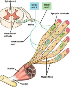
Figure 2.2: Motor Unit: a Motor Neuron with several branches, each one of them termi-nating at different muscle fibers of the same type. This terminal branches are typically in a ‘One-To-One’ relationship with the muscle fibers (a muscle fiber receives only a termi-nal branch, and a termitermi-nal branch innervates only a muscle fiber) [2,3,4].

An Action Potential (AP) is an electrical signal conducted along muscle fibers by which information is conveyed in the nervous system by means of ionic transport along the membrane. The combination of theseAPs along all the muscle fibers of a singleMUis called theMUAP[35].CNSsends this electrical signal which reach theα-MN responsible for initiating muscle contraction and spreads across muscle fibers, as a result of a series of electrically measurable de-polarization and re-polarization events (AP). If the nerve impulse arrives more often, the intensity of muscle contraction is greater [2]. Figure 2.3 shows a schematic representation of a single action potential.

Figure 2.3: Response to a single stimulus as a result of a single twitch contraction, which may last 25-75 ms [2].

(35)

associated to mechanical summation: as a result of higher stimulation regularity, the generated muscle force increases. Therefore, a sustained contraction (tetanus) results from a sequence ofAP[2].

The overall resultant muscular contraction strength hinges upon the number ofMUs recruited, as well as on the firing rate of the already recruited Motor Units (typically between 8 Hz to 35 Hz). Furthermore, according to the Henneman size principle, Motor Units are recruited according to their size in a voluntary contraction (first are recruited smaller MUs, being progressively larger MUs recruited with increasing muscle force) [2,36,37].

2.1.3 Electromyography (EMG)

The EMG signal is a biomedical signal which measures electrical potentials related to ionic currents (electrical activity of the muscle cell membrane) generated during muscle contraction. It represents neuromuscular activities and reflects the linear propagation of APs along the muscle fibers, depending as well from the anatomical and physiological properties of the muscles [2,35]. The spatial and temporal algebraic sum of potential con-tributions from the active Motor Units can be acquired with electrodes, which measure an electric difference of potential as a function of time, due to the property of superposition of electric fields [34, 3]. These electrodes may be needle electrodes invasively inserted directly into the target muscle tissues (which measure a single fiber or a small number of fibersAPs), or surface electrodes (non-invasive), attached to the skin surface (which measure the overall effects of theAPgenerated in the muscle fibers underlying the skin) [25,2,35].

Since electrical activity is affected by alterations in theMU’s structure,EMGis often used as a diagnostic tool [26].sEMGwill be used in this work. Complexity, randomness, nonstationarity (statistical proprieties change over the time) and nonlinearity (muscle activity andEMGsignal pattern don’t exhibit a linear relationship) are some of the main characteristics of thesEMGsignal [25]. Therefore, this signal presents a complex nature, with both structured (i. e. Motor Unit Action Potentials) and random-like (i. e. neural innervation) contributions [23].

(36)

2. THEORETICAL BACKGROUND 2.2. Technical base

2.2 Technical base

2.2.1 Signal acquisition

The EMGsignal is recorded using a bioPLUXresearch unit. Four pairs of electrodes are placed along the muscles, and data is collected by ipsilateral (electrodes positioned on the same side of the body) and contralateral (electrodes positioned on opposite sides of the body) acquisitions, while subjects perform a specific task. However, only ipsilateral analysis is executed (data collected from each arm of a subject will be analyzed sepa-rately). Data is collected from the first dorsal interosseus and extensor digitorum from each side of the body.

The device has eight analog channels with 12-bit resolution and also an external chan-nel to be used as a reference ground, and is used a sampling frequency of 1000 Hz. To ensure there is no loss of information, sampling frequency must be at least twice the signal’s maximum frequency (Nyquist sampling theorem) [34,38].

2.2.2 Low-level signal processing

ThesEMGanalogue signal (continuous in time) has to be converted into a discrete digital signal and analyzed both in time and frequency domains. Hence, the signal is usually rectified (the signal is transformed into its absolute value) and filtered (a specific range of frequencies will be attenuated and only the passage of the frequency of interest is allowed).

2.2.3 High-level signal processing

In order to characterize thesEMGsignal, Coherence,PLF,FD,LZ,DFAandMSE meth-ods, as well as a classification algorithm were used. These methods are described below.

2.2.3.1 Coherence

Neuronal synchrony can be analyzed by frequency analysis. Therefore, it is necessary to perform the cross-correlation in frequency domain between two distinct signals, being coherence the main linear dependence (correlation) measure in the frequency domain. However, this measure does not provide the two signals’ direction of interaction (direct coherence) [17,18,39]. Considering two signalsxandy (e. g. rectified and normalized

EMG signals stationary zero mean time series) at frequency λ, coherence can be com-puted using auto-spectra –fxx(λ) andfyy(λ)– and cross-spectra –fxy(λ) – estimations

by averaging discrete Fourier transforms of non-overlapping data segments taken from each signal. Eq. 2.1 expresses the coherence function,|Rxy(λ)|2, defined as the absolute

(37)

|Rxy(λ)|2=

|fxy(λ)|2

fxx(λ)fyy(λ)

(2.1)

Coherence function estimates values from0to1, assuming the value 0 if there is no

association between the two signals at that frequency, and the value 1 if there is a per-fectly linear association between them [19,17,39]. The strength and range of frequencies of common rhythmic synaptic inputs dispersed across a motoneuron pool may be quan-tified with coherence estimations [19].

2.2.3.2 Phase Locking Factor (PLF)

PLFis a measure of synchronization between two signals. Considering oscillatory time series, it is possible to obtain meaningful phase values, which can be used as synchro-nization indicators. TheEMGsignal, as the majority set of measurements available from real-world applications, assumes real values. However, in order to analyze a signal’s phase, it is suitable to convert the real-valued signal into a set of complex-valued data. Therefore, it is required the application of a transformation to extract the rotation angle over the time by projecting the time series onto a circumference [40,41,42].

Before the phase reconstruction procedure (which is only valid if the signal com-prises a clear oscillatory component), the presence of oscillatory activity may be assessed through the observation of significant values in the power spectrum. The frequencies of interest are then isolated by the application of a band-passed filter at a narrow band centered at each frequency. It is obtained an oscillatory signal from which the phase, or rotation angle, can be defined in the complex unit circle. In this work the method used to perform this task is based on the application of the Hilbert transform. Phase correla-tions between signals can then be studied, and correlation indices (e. g. phase coherence) can be computed in order to evaluate the strength of phase locking between two signals. The number of oscillation cycles considered influences this analysis. For a stationary time series, more oscillatory cycles (i. e. longer observation times) provide more reliable estimates while shorter observation times may lead to the concealment of important in-teractions (e. g. if they are weak or masked by noise). For a nonstationary time series, long observation times may not capture the presence of transient interactions [40].

Given two signalsj andk, with phasesφj(t) andφk(t)respectively, fort = 1, . . . , T

(beingT the number of discrete samples, i. e. the observation period),PLFbetween these two signals is defined by eq. 2.2 [41,42]:

ρjk ≡ | 1

T

X

t=1

ei[φj(t)−φk(t)]_|₌_|h_ei[φj(t)−φk(t)]_i| (2.2)

PLF ranges from0 to 1. Whileρjk = 0 corresponds to asynchronous signals (their

phases are not correlated),ρjk = 1 is attained if the two signals are in perfect

(38)

the two signals’ phase difference is strongly or weakly clustered around some angle in the complex unitary circle [41,42].

In this work,PLFbetween two signals will be calculated for moments of steady con-traction, where oscillations are expected.

2.2.3.3 Fractal Dimension (FD)

Fractal dimension’s concept arose from the need of a quantity other than length to dis-tinguish numerous degrees of complication for a geographical (statistically self-similar) curve, as described in [43] byB. B. Mandelbrot. When a straight ruler is used to mea-sure a country’s coastline, different estimates of its dimension are obtained according to the scale applied to the ruler, i. e., according to the ruler’s resolution. In other words, smaller rulers (higher resolutions) provide larger coastline measures. Hence, the concept of length becomes meaningless for geographical curves [43].FDis then used, for instance, to describe an object extremely detailed to be one-dimensional, whereas too simple to be two-dimensional.

EMG, Electroencephalogram (EEG) and Electrocardiogram (ECG) are complex medi-cal biosignals in which small smedi-cale structures (signal patterns) exhibit self-similarity with larger scale structures. This self-similarity phenomenon, which occurs with fractal scale relationship, can be described as the scale invariance of a process, and can be determined by the application ofFD[20,21,44]. In other words, fractal objects resemble each other in-dependently of the visualization scale or magnification. Altering the measurement scale and measuring changes in the curve’s length allows an estimation of theFD[20]. These fractals properties are expected to be found in asEMGsignal since the source of thesEMG recordings are similarAPs [20].

Despite the existence of multiple definitions forFD, such as Hausdorff dimension, correlation dimension, Higuchi dimension, box dimension, information dimension, among others, they are usually characterized by a non–integer fractional number [21,25,44].

It is documented in literature [21,22] thatFDfor physiological signals is more accu-rately estimated using Higuchi algorithm for non-periodic and irregular time series. In case of small number of data, this algorithm gives a reasonable estimation ofFD[25]. The Higuchi method has been successfully tested with the upper-limbs movement [25].

In order to apply the Higuchi method, it is firstly defined a new time seriesX_kmfrom a signal sampled at a fixed sampling rate,x(n) =X(1), X(2), X(3), . . . , X(N), as showed in eq. 2.3 [21,25,22]:

X(m), X(m+k), X(m+ 2k), . . . , X(m+⌊(N −m

k )⌋ ·k) and m= 1,2, ..., k (2.3) Wheremrepresents the initial time andkthe interval time, and they are both integers. Then the length of the curveXm

(39)

Lm(k) = [

⌊N−m

k⌋

X

i=1

|X(m+ik)−X(m+ (i−1)k)|] (N −1)

⌊(N−m_k )⌋ ·k

k (2.4)

Where⌊⌋denotes the Gauss’ notation. The average value overksets ofLm(k)is the

curve’s length for the time intervalk,hL(k)i. The curve is fractal with the dimensionD ifhL(k) ∝ k−Di. Afterwards, the linear relationship betweenL(k) andkis plotted in a log-log graph, and anFDestimation for a statistical self-similar curve can be obtained from the slope of the plotted line [21,25,22].

As previously referred, another definitions ofFDmay be used, however they will not be described in this work.

Another important feature is Maximum Fractal Length (MFL), which is the signal’s length (over unit time) measured from the logarithmic plot determiningFDat the small-est scale.MFLvalue is significantly influenced by singularities originated from the prox-imal muscles, since background activity has smaller magnitudes and for this reason doesn’t influence MFL so greatly. Since the density of singularities within a signal is related toMFL, this feature indicates the Motor Unit Action Potentials (MUAPs) rate in asEMGsignal, which is a more direct measure of the relative strength of muscle contrac-tion [21,22].

2.2.3.4 Lempel-ziv (LZ)

The LZ complexity measure can be used to analyze the deterministic complexity of a highly non-linear deterministic and chaotic setting [23]. In other words, this feature is used to evaluate finite sequences randomness and has been applied to evaluate the de-gree of complexity of biomedical signals, includingEMG[24].

In order to compute theLZmeasure, thesEMGsignal,x(i)(or any other discrete time

signal ofN samples) must be converted into a symbolic sequence, s(i), conventionally a binary sequence, by comparison with a threshold. Thus, if thesEMGsignal is smaller than that threshold, the signal takes value 0, otherwise, it takes value 1, which is mathe-matically expressed by eq. 2.5. Eq. 2.6 represents the symbolic sequenceS[23,24,45].

s(i) =

(

0, ifx(i)<threshold

1, otherwise (2.5)

S=s(1), s(2), ..., s(n) (2.6)

Afterwards, it is determined the number of different patternsP contained in the se-quenceS. In order to do that, it is necessary to denote [23,24]:

1. The length of the symbolic sequenceS:N

(40)

sequence is converted:β(for a binary sequenceβ = 2)

3. A collection (designated as vocabulary) of all of the substrings that belong to the sequenceS:v(S)

4. Two distinct substrings of the sequenceS:Q=s1, s2, . . . , sqandR=sq+1, sq+2, . . . , sq+r

5. A concatenation of the substringsQandR: QR=s1, s2, . . . , sq+r

6. A substring of the sequence S derived fromQRafter the removal of its last charac-ter:QRπ=s1, s2, . . . , sq+r−1

The scanning process begins with the initialization of the sequencesS,RandP (S=

s1,R =s2 andP = 1), being the symbols1 the first pattern. Afterwards, it is added to the substringRa new subsequent element,si, of the sequence S untilR doesn’t belong

to v(QRπ). Hence, if the sequenceR doesn’t belong tov(QRπ), R is defined as a new distinct pattern of the sequenceS and the sequenceP is increased by one. Then,Qand Rare reset (Q=QRandRtakes the value of the subsequent elementsiofS) for the next

iteration. This process continues untilQR=S[23,24].

For example, applying this method in a binary sequence (with two symbols,0,1,β= 2)1,0,1,1,1,0,1,0, it would be obtained the parsed sequence1.0.11.10.10, where distinct

patterns are separated by a period. In this exampleP = 4[23].

Finally, afterP has been found, this sequence is normalized by the number of char-acters β and the length, N, of the sequence S, as expressed by eq. 2.7, being Cβ the

normalizedLZcomplexity value ofS[23,24].

Cβ =

Plog_β(N)

N (2.7)

In this work will be used a binary sequence.

2.2.3.5 Detrended Fluctuation Analysis (DFA)

Detrended Fluctuation Analysis is frequently used as a nonlinear analysis method or a fractal time series algorithm, being typically applied to noisy signals, since it is an im-portant tool in the detection of long range correlations. This is a very advantageous method, since it combines the advantages of both time domain and time-frequency do-main features.DFAalso outperforms spectral analysis features, such as Discrete Wavelet Transform and Wavelet Packet Transform [25].

TheDFAmethod can be applied to the study of electrophysiological signals, being a modified Root Mean Square (RMS) analysis of a random walk. In order to describe this method’s procedure it is necessary to denote{x(t)}as thesEMGtime series, beingtthe discrete time in the range[1, N](N is the time series’ sample length) [25].

First thesEMG signal is integrated in order to be converted into random walk. Eq. 2.8 expresses this integrated series (also known as profile or cumulative sumy(k)), being

(41)

y(k) = k

X

t=1

[{x(t)} −x(t)], k= 1, ..., N (2.8)

Then these integrated series are parted intoLidentical windows (box sizes) and each window has an n time point. This point, n, is a DFA parameter, and it is the largest integer smaller thanN divided byL[25].

Afterwards, a least-square fit is applied to the integrated series {y(k)} within each window, being each window’s least-square line the semi-local trend within that window. This is anotherDFAparameter. After this, the integrated series and the detrended time seriesRMSfluctuation is computed. This is given by eq. 2.9, whereyn(k)is they coordi-nate coefficient [25]:

F(n) =

v u u t 1 N N X k=1

[y(k)−yn(k)]2 (2.9)

Finally, this calculations are repeated for every window, in order to obtain the log-log graph of the linear relationship betweenF(n)andn. The common base 10 logarithm is applied, and the fluctuation showed in the graph is characterized by the slope of the line which relateslogF(n)tologn. This slope is theDFA’s scaling exponent αwhich is the power law (fractal) scaling.αis a self-similarity parameter and is given by eq. 2.10 [25]:

α= [∆ log10(F(n))]

[∆ log₁₀(n)] (2.10)

TheDFA’s scaling exponents assume values between0and2. According to its value

the time series behavior can be explained. Therefore:

• If0< α < 1₂ the time series is anti-correlated

• Ifα ∼= 1₂ the time series is uncorrelated, or indicates white noise (the value at one

instant cannot be correlated with any previous value)

• If 1

2 < α <1the time series is correlated • Ifα∼= 1indicates pink noise (1_f noise)

• If1< α < 3₂ indicates nonstationary or random walk

• Ifα∼= 3₂ indicates Brownian noise (i. e. the integration of the white noise)

This value is related to theFDparameters by a linear relationship, since larger scale exponentαvalues correspond to smallerFD[25].

(42)

The window function depends on the maximum and minimum window size and the function’s increment interval. In literature [25] are proposed experiment suggestions for the first two parameters. The adjacent interval can be defined as an arithmetic progres-sion or as a geometric progresprogres-sion. For the fitting procedure, different types of polyno-mial fits can be used (linear, quadratic, cubic and so on).

2.2.3.6 Multiscale Entropy (MSE)

Entropy has been often used to quantify complexity, since traditional entropy definitions (e. g. Shannon-entropy) are used to measure disorder and uncertainty, as well as to characterize a systems’ gain of information [28]. Approximate Entropy and its modifica-tion Sample Entropy are entropy-based complexity measures with a single scale which are widely used in short and noisy time series. Based on these two features, Multiscale Entropy (MSE) has been introduced [27,28,46].

In order to compute the Sample Entropy it is necessary to denote:

1. The time seriesx(i) ={xi, xi+1, xi+2, . . . , xN}of lengthN [27,28,46];

2. Two m-dimensional sequence vectors, y(m)₍_i_{) =} _{_x

i, xi+1, xi+2, . . . , xi+m−1} and

y(m)₍_j_{) =}_{_x

j, xj+1, xj+2, . . . , xj+m−1}. These vectors are embedded from the time seriesx(i)in a delayedm-dimensional space. They are considered similar (i. e. they match) if their distance is smaller than a tolerancer[27,28];

3. The probability (density)ρm₍_r₎ _{of two vectors match in the}_m_{-dimensional space,}

which is calculated by counting the matched vector pairs’ average number. This probability is also computed for the embedded dimensionm+1, in order to estimate

ρm+1₍_r₎_[₂₇_].

Therefore, Sample Entropy is defined according to eq. 2.11:

SampEn(m, r) = log[ ρ

m₍_r₎

ρm+1₍_r₎] (2.11)

In order to obtain theMSE, the simple "coarse-grained" multiscale approach is applied on the original time series, x(i), before the entropy measure. x(i) is then segmented

into N

τ coarse-grained sequences with length τ, and the mean value is calculated for

each segment. Eq. 2.12 shows the new coarse-grained time series, {vj(τ)}, whereτ = 1,2,3, . . . [27,28].

vj(τ) = 1

τ

jτ

X

i=(j−1)τ+1

xi, 1≤j≤

N

τ (2.12)

(43)

approach introduces linear smoothing (the high frequency components are gradually re-moved of the original time scale) and decorrelation between the vectors [27,28,46]. Fur-thermore, Entropy decreases with the scale factor concerning White noise, remaining constant for all scales regarding 1/f noise (correlated fluctuations), which is consistent with the fact that 1/f noise is more complex than White noise [47].

The two free parametersm(the sequence length) andr(the tolerance level) are asso-ciated with the likelihood of two sequences of lengthmstay close to one another at the next step within a certain tolerance levelr. Consecutive sequences are identical when the output is zero. Decreasing the tolerance level will increase the entropy value, since it will be harder to find consecutive sequences close together within the given tolerance level. Therefore, both of the parameters aren’t absolute measures [28]. In literature [28] it is proposed to usem= 2andr = 0,15σ, beingσthe standard deviation of the original time series.

It is important to reference that in the multiscale approach, increasing the value ofτ will decrease the data variation. Also, the tolerance value is assumed to be the same for all scales (the standard deviation value is not adjusted for each scale), reason why the standard deviation value of a given data set diminishes whenτ increases. However, it doesn’t exist a general relationship between standard deviation and the entropy, being that relationship dependent of the correlation properties [28].

2.2.4 Classification

Classification methods are used in order to identify the belonging of a novel observation in a set of categories (sub-populations). These categories are obtained with basis in a training group of observations. It is necessary to have previous knowledge of the cate-gory membership of each observation of the training group. These observations are then analyzed in various levels, according to the used features (quantifiable properties). In this project, the used features are: kurtosis, maximum frequency, mean, median frequency, power band, spectral kurtosis, spectral skewness, spectral spread and correlation. There will be also analyzed the results of the previously referred implemented algorithms (co-herence,PLF,FD,LZ,DFA andMSE). Classification can be implemented throughout a various number of algorithms, the classifiers, described below. Leave-one-out cross val-idation iterator is used to split data in train/test sets. Hence, all samples except one are used as a train set, being this left out sample tested after [48].

2.2.4.1 k - Nearest Neighbors

(44)

2.2.4.2 Decision Tree

A Decision Tree is a hierarchical tree structure based on a series of rules concerning the attribution of classes to the input sample data. This structure consists of a root node, in-ternal and exin-ternal nodes, connected by branches. Each inin-ternal node (nonleaf node) is concomitant with a decision function in order to determine the following node, splitting the value into different branches corresponding to different attributes, whereas each ex-ternal node (leaf node) denotes a class. Generally, the Decision Tree algorithms procedure consists in two steps: tree building and tree pruning [50,32].

2.2.4.3 Random Forest

The Random Forest algorithm is applied toKsamples drawn with replacement from the training group (bootstrap samples). Then, unpruned regression trees are built for each bootstrap sample. When splitting a node during this tree construction, it is chosen the best split among a random subset of features (i. e., the algorithm randomly samples p0 (0< p0 < p) of theppredictors (input variables)), instead of the best split among all the predictors. Finally, the predictions of theK trees are averaged, in order to predict new data [48,33].

2.2.4.4 AdaBoost

The AdaBoost method uses a linear combination (ensemble) of several weak classifiers (simple decision rules) which when combined originate a strong classifier (decision rule more complex and accurate). This sequence of weak classifiers is applied to repeat-edly modified versions of the data set. These modifications consist in the application of weights (wi = w1, w2, . . . wN) to each sample of the training group. In the first

itera-tion the weak classifier trains on the original data set (all the weights are initially set to wi = _N1). The data set is reweighted for each successive iteration: the weights of

incor-rectly predicted training examples at previous iterations increase, while the weights of correctly predicted training examples decrease. Hence, the subsequent weak classifier is obliged to focus on the missed examples of the previous weak classifier [48,29].

2.2.4.5 Naïve Bayes

The Naïve Bayes technique is based on the application of the Bayes theorem with the naïve presupposition that every pair of features is independent. Defining y as a class variable andxi =x1, . . . , xnas a dependent feature vector, the classification rule defined

byyˆ= arg maxyP(y)Qn

i=1P(xi|y)can be followed. Therefore, the maximum a posteriori

(45)

3

Acquisition Methods

3.1 Subjects

(46)

3. ACQUISITIONMETHODS 3.2. Acquisition Protocol

3.2 Acquisition Protocol

The performed task, visible in Figure 3.1, was repeated for 6 minutes or less according to maximum time borne by the patients. Subjects sat down and placed both hands and forearms on a desk in a parallel position, 10 cm away from each other with hand palms facing one another in 90 degrees flexion with the elbow. While listening to a programmed sound, which guided the movement, subjects were asked to coordinately elevate both index fingers vertically with maximum articular amplitude in an opposite direction from the other fingers position, hold that position for 3 seconds while maintaining a certain force and return to the original position, remaining in that position for 3 seconds while trying to relax the arms muscles as much as possible.

3.3 Recording

As previously stated, contralateral and ipsilateral acquisitions were recorded simultane-ously, and 4 signals were acquired from each subject (with the exceptions specified in section 3.1) using EMG sensors attached to a bioPlux device (device specifications ex-plained in section 2.2.1). Each sensor has two connected electrodes. The sensors were placed on the first dorsal interosseus muscle for both left and right hand, and on the ex-tensor digitorum communis muscle for both left and right forearm. Ground was placed on ulna bone inferior extremity, where no muscle activity is present. Figure 3.1 shows the surface electrodes placements. Trying to better isolate moments of contraction, two accelerometer sensors were placed in the index finger, being acquired two signals for the z axis, one for the left and another for the right hand. These signals were only acquired for some subjects from the patient and the control groups, since this procedure did not demonstrate to be efficient.

(a) (b)

(47)

4

Signals Processing

4.1 Low-level Processing

All acquired signals were processed using python language. First, the signals’ ampli-tude was converted from ’bins’ into ’mV’ and its Direct Current Component (DC) was removed. Then, it was applied a third order butter band pass filter of 10 – 500 Hz. From each pair of ipsilateral signals, intervals of common contraction were isolated from inter-vals of relaxation. It is not possible to predefine a common onset value to all signals due to the differences among each subjects’ signals, as well as the different amount of noise inherent to each one of the signals. The used algorithm is explained in [51]. From this algorithm result an onset (beginning of an activation) and an offset (ending of an acti-vation) for each contraction, which is different among the signals collected from the left and from the right arms. However, since the analysis is made for ipsilateral acquisitions, and assuming that subjects performed the task properly, without exerting any unrelated contractions regarding the task, it is possible to find the onset values for the hand and use those same values for the forearm as well.

4.2 High-level Processing

(48)

4. SIGNALSPROCESSING 4.2. High-level Processing

posterior averaging of all epochs. FD,LZ,DFAandMSEcalculus was applied to a con-catenation of all contractions.

4.2.1 Coherence Processing

Prior to coherence calculus, allEMGsignals were full-wave rectified and then, for each contraction, coherence was calculated using matplotlib.mlab.cohere tool. Coherence is then calculated for an average of these moments of contraction. The used sampling fre-quency is 1000 Hz, theNFFTis 512 and the value that dictates the dependency between Fast Fourier Transform (FFT) windows isNFFT/2. NFFTvalues are related to frequency resolution, and more precision in frequency resolution is obtained for higher values of NFFT or lower values of sampling frequency. Therefore, for a sampling frequency of 1000 Hz, making NFFTas 512 yields a resolution of 1.95 Hz. For NFFT 4096, resolu-tion would be 0.244. Coherence was averaged for each frequency among all the subjects within the same group. The following coherence tests were also made for a few members of both groups:

• For the same signal, compute coherence for the first 10, the first 20, the first 30, and so on, until the total length of the signal be achieved, in order to analyze the influence of the signal’s length in coherence calculus.

• For the same signal, compute coherence for only 10 contractions, from 10 in 10 contractions, along the whole signal’s length, in order to analyze coherence over time.

• For the same signal, compute coherence per contraction and per relaxation, in order to analyze coherence over time.

• Compute coherence for the concatenation of all contractions, to analyze coherence with higherNFFTvalues.

• Find the frequency associated to the maximum value of coherence for frequency band, in order to analyze variability among subjects within the same group.

4.2.2 PLF Processing