Manager skill or luck? Assessing active management decisions through attribution analysis

MASTER

M

ATHEMATICAL

F

INANCE

M

ASTER

’

S

F

INAL

W

ORK

INTERNSHIP REPORT

MANAGER SKILL OR LUCK? ASSESSING ACTIVE MANAGEMENT

DECISIONS THROUGH ATTRIBUTION ANALYSIS

P

AULO

G

ABRIEL

G

ÓIS

M

OREIRA

MASTER

M

ATHEMATICAL

F

INANCE

M

ASTER

’

S

F

INAL

W

ORK

INTERNSHIP REPORT

MANAGER SKILL OR LUCK? ASSESSING ACTIVE MANAGEMENT

DECISIONS THROUGH ATTRIBUTION ANALYSIS

P

AULO

G

ABRIEL

G

ÓIS

M

OREIRA

SUPERVISORS:

A

I

B

J

H

i

Abstract

Some say trading is just like gambling in a casino: there can be certain techniques, but the most important factor is luck. I have come across more than a handful of people stating similar assertions. How can there be portfolio managers such as Blackrock or J. P. Morgan with such reputation and so many clients? How is it that they reach better results than other managers do, consistently over time?

This report does not provide a direct answer to the above question. However, it compiles the knowledge acquired over a three-month internship at Mercer related to performance measurement and its use to analyze the sources of excess return relative to a benchmark. The following dissertation has been written with the belief that a consistent positive excess return over time is an indicator of manager skill (Christopherson et. al., 1998).

In practical terms, daily calculations of performance and risk measures provided a deeper understanding on the financial theory and the actual methods used in a professional environment.

In this document, Chapter 1 introduces the basics about the internship and its purpose. Chapter 2 presents a description of the tasks undertaken at Mercer and the financial theory behind them. Chapter 3 contains a practical case of attribution analysis. Chapter 4 holds the main conclusions.

Keywords: Performance Attribution, Attribution Analysis, TWRR, Benchmark, Allocation Effect, Selection Effect, Funding Level, Risk Measures

ii

Acknowledgments

To my parents, for their constant and unconditional support, and for reminding me to finish what I have started.

To Mercer, for accepting me in the team and providing all necessary means to understand the nature of performance reporting. And to everyone in the PRT team, and those who challenged me to always give the extra mile.

To my supervisors, for their amazing patience. To Madalena and Jessica, for providing me with the right contacts and necessary financial theory to complete this internship report. Without them, none of this would have been possible.

To all my friends, for so many good laughs we had and many more to come!

And of course, to my wonderful cousin, Sophie, whom I will always cherish so much.

iii

Table of Contents

1. Introduction ... 1

2. Theory ... 3

2.1 Performance measurement ... 3

2.1.1 Time-Weighted Rate of Return ... 3

2.1.2 Modified Dietz ... 4

2.1.3 Money-Weighted Rate of Return ... 5

2.1.4 Benchmarks, Benchmark Construction and Rebalancing ... 5

2.2 Performance Attribution Analysis ... 7

2.2.1 Return Attribution Analysis – Introducing the Brinson-Hood-Beebower Model ... 7

2.2.1.1 Allocation and Selection Effects ... 7

2.2.1.2 Interaction Effect ... 8

2.2.1.3 Contrasting BHB and BF models ... 9

2.3 Risk Attribution Analysis ... 10

2.3.1 Standard Deviation and Beta ... 10

2.3.2 Measures of Excess Return ... 10

2.4 Performance Appraisal ... 11

2.5 Mercer Manager Ratings ... 12

2.6 Pension Funds and De-Risking Delegated Solutions: A Brief Review ... 13

3. Results and discussion ... 15

3.1 Day-to-day tasks ... 15

3.2 Results ... 15

3.2.1 The Scheme ... 15

3.2.2 The portfolio and the benchmark ... 17

3.2.3 BHB and BF Models ... 22

3.2.4 Risk Attribution Analysis ... 25

4. Conclusion ... 28

5. References ... 29

iv List of Figures

FIGURE 1 – Funding level progression ... 16

FIGURE 2 - Assets and liabilities progression since inception ... 30

List of Tables TABLE 1 – Overview of the portfolio as at 31-12-2014 and 31-12-2018 ... 16

TABLE 2 – Overview of the portfolio asset allocation as at 31-12-2014 ... 17

TABLE 3 – Overview of the portfolio asset allocation as at 31-12-2018 ... 17

TABLE 4 – Performance by asset class as at 31-12-2014 ... 18

TABLE 5 – Target growth allocation ... 20

TABLE 6 – Total growth returns (excluding passive funds)... 21

TABLE 7 – Attribution analysis – application of BHB and BF models at at 31-12-2014 ... 22

TABLE 8 – Attribution analysis – application of BHB and BF models at at 31-12-2018 ... 23

TABLE 9 – Attribution analysis – top and bottom contributors using BHB and BF models ... 24

TABLE 10 – Attribution analysis – main risk measures as at 31-12-2014 ... 25

TABLE 11 – Attribution analysis – main risk measures as at 31-12-2018 ... 27

TABLE 12 – Actual asset allocation of the growth and matching portfolios as at 31-12-2014 ... 30

TABLE 13 – Actual asset allocation of the growth and matching portfolios as at 31-12-2018 ... 32

1

1. Introduction

The Master of Mathematical Finance at ISEG-UTL (Lisbon School of Economics and Management) provides its students with the possibility to further study a specific area of knowledge among the courses lectured as part of the programme. Three ways are proposed as the Master’s Final Work: thesis, project, or internship report, the latter being presented here.

The writing of this report has three purposes. First, it is not a simple outline but rather a written description of the activities performed along the internship and a reflection upon them. Secondly, it is a delineation of their theoretical framework. And thirdly, it is a link between theory and practice, and a dichotomy between academic models and their application in the financial world.

As a means of developing my personal interests regarding the Master’s programme, the opportunity of joining Mercer’s Performance Reporting Team (PRT) as an intern was ideal. Its methods are modern and require both financial knowledge and a practical orientation towards computer software.

Mercer is a consulting firm that specializes in the health, wealth and career wellness of people. As an inherent part of wealth, the PRT monitors investments that result from pension plans administrated by Mercer. These investments are made directly by Mercer or other managers, which are meticulously selected using a set of techniques and considering the success of each manager, which shall be called “skill”, in contrast to luck.

Mercer is a company of Marsh & McLennan Companies (MMC) and has c. 300 workers in Lisbon. It provides each client with strategic investment solutions to meet their funding level1 _{objective. The internship took place at}

Mercer’s office in Lisbon, between April 26th _{and September 8}th _2017.

The aim of this internship was to acquire an actual understanding of the main performance measures and how to use them in performance appraisal through attribution analysis, while having a first contact with the financial world. The activities have been written down along the internship and the related

1 _{Funding level: quotient between the assets and the liabilities of a pension plan. The long-term objective}

2

theory has been generously provided by certified colleagues (CFA, CIPM) at Mercer itself. However, no reference to real clients shall be made in this report as part of Mercer sigil. Instead, imaginary portfolios, in the bounds of reality, will be presented, without loss of rigorousness.

Hence, the purpose of this study is to research and evaluate the theory and practicalities of performance calculations using the attribution analysis methodology at Mercer.

3

2. Theory

Performance evaluation allows financial analysts to understand more on the return and risk of investments portfolios over specified periods of time, and is composed of three essential topics: performance measurement, attribution and appraisal. It is a set of powerful tools that help investors assess the quality of active investment management.

2.1 Performance measurement

In this chapter, basic concepts of performance measurement are presented. Let us start with the definition of rate of return.

The rate of return of an investment is defined as the percentage of variation in wealth as a result of holding the investment over a certain period of time. However, as objective as this definition may seem, cash-flows must be taken into account to have a rate that properly reflects reality.

2.1.1 Time-Weighted Rate of Return

To effectively compare different rates of return, it is important that the measure should be insensitive to cash-flows (manager’s perspective). However, a client may want to know how the portfolio performed considering withdrawals and deposits (client’s perspective). The time-weighted rate of return (see, for example, Elton et al., 2017) is hereby presented and gives an approximation of the rate of return of an investment, taking away the impact of external cash-flows:

𝑟

=

𝑀𝑉₀+𝐶𝐹 (1)

Where

𝑟₁ = Rate of return at end of period 1 𝑀𝑉𝑡 = Account’s market value at time 𝑡

4

The formula of the compound annual growth rate will be useful to achieve some performance measures along the practical work, with k being the number of years:

𝑟 = ∏ (𝑟𝑛𝑖 𝑖 + 1)1 𝑘⁄ − 1 (2)

To calculate the performance of a fund, it is essential to introduce the concept of Net Asset Value (NAV), which differs from the actual valuation of the fund:

𝑁𝐴𝑉 = 𝐴𝑠𝑠𝑒𝑡𝑠−𝐿𝑖𝑎𝑏𝑖𝑙𝑖𝑡𝑖𝑒𝑠

𝑁𝑢𝑚𝑏𝑒𝑟 𝑜𝑓 𝑂𝑢𝑡𝑠𝑡𝑎𝑛𝑑𝑖𝑛𝑔 𝑆ℎ𝑎𝑟𝑒𝑠 (3)

An investor seeks to buy at a price that is lower than the NAV in order to make a profit.

2.1.2 Modified Dietz

The formula for the TWRR works only when the timing of cash-flows is available at the end of the period. If, for example, the portfolio experiences daily cash-flows but prices are provided on a monthly basis, one should use the Modified Dietz instead:

𝑟

=

𝑀𝑉_𝑡𝐵+∑𝐼𝑖=1(𝐶𝐹𝑖,𝑡∗𝑤𝑖,𝑡)

(4)

Where 𝑤𝑖 = 𝐶𝐷−𝐷𝑖

𝐶𝐷 represents the fraction of the period over which

cash-flow 𝑖 applies,

𝐶𝐷 = Total number of calendar days in period 𝑡

𝐷𝑖 = Calendar days from beginning of period to cash-flow

𝑀𝑉_𝑡𝐸 = Valuation at the end of period 𝑡 𝑀𝑉_𝑡𝐵 = Valuation at the beginning of period 𝑡 𝐶𝐹_𝑖𝑡 = Cash-flow 𝑖 that occurred during period 𝑡

5

Originally, Dietz (1966) proposed to subtract half the value of cash-flows at the end of the period and add the other half at the beginning of the period to reach an approximation of the real rate of return.

2.1.3 Money-Weighted Rate of Return

The formula for the Money-Weighted Rate of Return (MWRR) is slightly different, since we want contributions to be taken into account – see, for example, Haugen (1997). In the context of pension funds, swung prices are those that reflect contributions made over the period of investment. The formula for the return is given below:

𝑀𝑉₁ = 𝑀𝑉₀(1 + 𝑅) + ∑𝐼 𝐶𝐹_𝑖(1 + 𝑅)𝑊𝑖

𝑖=1 , (5)

𝑅 = Total rate of return.

2.1.4 Benchmarks, Benchmark Construction and Rebalancing

Before introducing the theory behind performance attribution, it is important to mention that it only makes sense when comparing a portfolio’s performance to a benchmark’s. First of all, a benchmark is defined as a measure against which a portfolio’s performance, risk and construction are assessed. If a portfolio is focused on a specific market, it is common to choose a market index. Otherwise, splitting among different asset classes is usually more adequate.

After assigning each asset class a benchmark, it is necessary to define a rebalancing frequency (quarterly, semi-annually…). This way, the portfolio keeps pace with the long-term strategic asset allocation.

Rebalancing is an important concept when benchmarks are composed of several asset classes, such as equities or bonds. It defines how the asset allocation drifts over time until a new rebalancing date is reached. It refers to the period between rebalancing dates and its frequency is usually monthly or quarterly.

6

𝑊_𝑖,𝑡+1̇ = 𝑊_𝑖,𝑡(1 + 𝐵_𝑖,𝑡+1) (6)

𝑊_𝑖,𝑡+1̇ = Weight of the benchmark in 𝑖 th sector before reweighting to 100% at time 𝑡 + 1

𝑊𝑖,𝑡 = Weight of the benchmark in 𝑖th sector at time 𝑡

𝐵_𝑖,𝑡+1 = Return of the benchmark in 𝑖th sector at time 𝑡

Reweighting to 100% yields:

𝑊_𝑖,𝑡+1= 𝑊_𝑖,𝑡+1̇ / ∑𝑛_𝑖=1𝑊_𝑖,𝑡+1̇ (7)

𝑊_𝑖,𝑡+1= Weight of the benchmark in 𝑖th sector at time 𝑡 after reweighting

The sum of the product of the benchmark split and the respective performance gives the total benchmark, 𝐵, for a certain sub period. Provided that ∑𝑛_𝑖=1𝑊_𝑖 = 1:

𝐵 = ∑𝑛_𝑖=1𝑊_𝑖𝐵_𝑖 (8)

The product of each sub period total benchmark gives the period total benchmark.

Likewise, the formula for the portfolio return is given by:

𝑅 = ∑𝑛𝑖=1𝑤𝑖𝑅𝑖 (9)

𝑅𝑡 = Rate of return at time 𝑡

7

2.2 Performance Attribution Analysis

Performance attribution is a set of techniques used to identify and quantify the sources of excess return and respective risk of a portfolio against its benchmark in order to understand the consequences of active management decisions. It includes both return and risk attributions. While return attribution aims to classify the sources of excess return due to investment decisions, risk attribution focuses on the risk of such decisions.

2.2.1 Return Attribution Analysis – Introducing the Brinson-Hood-Beebower Model

The Brinson-Hood-Beebower (BHB) model (Brinson et. al., 1986) arises from the investors’ need to decompose the sources of excess return relative to a benchmark. These can be decomposed into allocation and selection effects.

Also, some individual investors have the money but not the time to invest directly through the financial market. Therefore, it is only natural for them to rank managers according to their skill and pick those in which they feel they could put their trust and capital.

2.2.1.1 Allocation and Selection Effects

Allocation effect assumes that each sector in the portfolio has the same return as the benchmark’s sectors. Only the impact of capital allocation to each individual sector is measured.

Every portfolio manager aims to allocate more of his/her disposable capital into a sector that is outperforming and less to a sector that is underperforming. This is commonly known as “timing”.

The impact of the asset allocation is measured through the difference between an allocation notional fund return and the benchmark return.

𝐵_𝑠− 𝐵 = ∑𝑛_𝑖=1𝑤_𝑖𝐵_𝑖 − ∑𝑛_𝑖=1𝑊_𝑖𝐵_𝑖 = ∑𝑛_𝑖=1(𝑤_𝑖− 𝑊_𝑖)𝐵_𝑖 = ∑𝑛_𝑖=1𝐴_𝑖 (10)

𝐵𝑆 = Notional rate of return of the benchmark

8

The sum of each sector contribution yields the total allocation contribution.

Stock selection assumes that each sector in the portfolio has the same weigh as the benchmark. Therefore, only the impact of security picking is measured. The difference between a selection notional fund and the benchmark return gives rise to the contribution from selection.

𝑅_𝑠− 𝐵 = ∑𝑛_𝑖=1𝑊_𝑖𝑅_𝑖 − ∑𝑛_𝑖=1𝑊_𝑖𝐵_𝑖 = ∑𝑛_𝑖=1𝑊_𝑖(𝑅_𝑖 − 𝐵_𝑖) = ∑𝑛_𝑖=1𝑆_𝑖 (11)

𝑅_𝑆 = Notional rate of return of the portfolio

The sum of the selection contribution within each sector yields the total selection contribution.

2.2.1.2 Interaction Effect

Attribution analysis aims to explain every source of excess return, 𝑅 − 𝐵, generated by the active investment decision making process. The sum of the allocation and selection effects should explain all the excess return. However, 𝑅_𝑠− 𝐵 + 𝐵_𝑠− 𝐵 = 𝑅_𝑠− 𝐵_𝑠− 2𝐵 ≠ 𝑅 − 𝐵. Therefore, the interaction effect is given by 𝑅 − 𝑅_𝑠− 𝐵_𝑠+ 𝐵 = ∑𝑛_𝑖=1(𝑤_𝑖 − 𝑊_𝑖)(𝑅_𝑖− 𝐵_𝑖).

This portion is not a residual, but rather an interaction between both allocation and selection effects. Finally, the general formula to calculate the excess return of a portfolio is presented below, with all components included:

𝑅 − 𝐵 = ∑ 𝑤_𝑖𝑅_𝑖 𝑛 𝑖=1 − ∑ 𝑊_𝑖𝐵_𝑖 𝑛 𝑖=1 − ∑ 𝐼_𝑖 𝑛 𝑖=1 = ∑𝑛 𝑤_𝑖(𝑅_𝑖− 𝐵_𝑖) 𝑖=1 + ∑𝑛𝑖=1(𝑤𝑖− 𝑊𝑖)(𝐵𝑖)− ∑𝑛𝑖=1(𝑤𝑖 − 𝑊𝑖)(𝑅𝑖− 𝐵𝑖) (12)

9

2.2.1.3 Contrasting BHB and BF models

Calculating the allocation effect may be misleading when a certain sector benchmark is negative. If we consider a negative sector benchmark and an overweight position, the allocation effect will be negative. However, that should not happen if the overall benchmark has performed worse than the sector benchmark. Overweighting a sector with a negative performance that has yet performed better than the overall benchmark should result in a positive impact. The Brinson-Fachler (BF) model (Brinson and Fachler, 1985) introduces a new formula to solve this problem:

𝐵𝑠− 𝐵 = ∑𝑛𝑖=1(𝑤𝑖 − 𝑊𝑖)(𝐵𝑖− 𝐵) = ∑𝑛𝑖=1𝐴𝑖 (13)

As a consequence, an overweight position to a sector with positive return that has underperformed the overall benchmark will generate a negative selection contribution.

10

2.3 Risk Attribution Analysis

Risk attribution helps investors in understanding the sources of risk of their portfolio. Return and risk attribution go hand-in-hand when analysing active investment strategies and provide a complete attribution analysis. Probably the most indispensable measure of risk is the standard deviation:

𝜎 = √

𝑛−1 (14)

For annualized standard deviation, we will be using 𝜎_{𝑎𝑛𝑛𝑢𝑎𝑙𝑖𝑧𝑒𝑑}= 𝜎√𝑡, where t is the number of periods in a year for returns that are independent over time. If returns are unstable over time, the standard deviation will likely be high, suggesting we are dealing with a riskier asset. On the other hand, if returns are more stable over time, standard deviation will be lower, suggesting a less risky asset.

𝛽 is also an important measure in risk attribution and is given by:

𝛽

=

𝜎_𝑚2

,

𝑅_𝑚 = Overall market return

𝛽 is a measure of how an asset moves compared to the market. While standard deviation can be interpreted as total risk, the beta coefficient can be interpreted as the non-diversifiable risk (see Tucker et al, 1994, or Fischer & Jordan, 1995).

2.3.2 Measures of Excess Return

One of the most widely used riskadjusted measure is the Sharpe ratio -see Sharpe et al., (1995). It gives an idea of the reward earned by the investor for each unit of risk he or she is willing to take:

11

𝑆𝑅 =

𝜎

,

𝑅𝑝 = Rate of return of the portfolio

𝑅_𝑓 = Risk-free rate of return

Tracking error, or tracking risk, measures the relative risk between a portfolio and its benchmark. It gives an idea of how well a portfolio is performing compared to a benchmark, and it is given by:

𝑇𝑅 = 𝜎(𝑅_𝑝− 𝑅_𝐵), (17)

𝑅𝐵 = Rate of return of the benchmark

Tracking error is very useful for passive managers since it gives an idea of how well the manager is tracking a benchmark. A manager that intends to outperform a certain benchmark will usually deal with higher tracking risks. This measure is also known as active risk since it yields the standard deviation for the series of differences between portfolio’s and the benchmark’s returns, thus evaluating the consistency of the excess returns.

Information Ratio is a risk-adjusted measure of the portfolio or investment returns that indicates how a manager is producing consistent excess return relative to a benchmark over time.

𝐼𝑅 =𝑅𝑝−𝑅𝐵

𝑇𝑅 (18)

Higher values of information ratio suggest that the manager was able to outperform the benchmark during the period, given a certain level of active risk.

2.4 Performance Appraisal

After all sources of return have been fully identified and quantified, performance appraisal helps to understand the ability of an investor that seeks to beat its benchmark. It is important to make an analysis that includes both

12

return and risk as to measure the worthiness of taking a certain amount of risk for the return that was earned.

Performance appraisal is the core of our work. It is what will answer the question: was the investor’s portfolio return the result of technical skill or sheer luck? Note that skill does not depend on time. Skill is persistent – see Sharpe et

al. (1999). It is the result of a series of returns that were successful in beating

their benchmark.

As an ending note to this chapter, a thorough performance appraisal also provides a stronger basis to an effective manager selection process.

2.5 Mercer Manager Ratings

Mercer provides a wide range of investment strategy research ratings (or simply ratings) that reveal Mercer’s opinion of investment strategies undertaken by different managers. Although Mercer takes other components into account, in this work we shall focus mainly on these measures of performance and risk, which are included in the category portfolio construction. It “refers to the manner

in which the manager translates investment ideas into decisions on which investments to include in a portfolio and what weightings to give to each of

these investments”2_.

Mercer defines ratings A and B+ as being investable strategies for its clients:

A Strategies assessed as having “above average” prospects of outperformance

B+

Strategies assessed as having “above average” prospects of outperformance, but which are qualified by at least one of the following:

• There are other strategies in which Mercer has a greater conviction that outperformance will be achieved

• Mercer requires more evidence to support its assessment

13

2.6 Pension Funds and De-Risking Delegated

Solutions: A Brief Review

De-risking Delegated Solutions (DDS) is a service at Mercer that provides its clients with a strategy plan that aims to reach 100% of the funding level in a given time period. Its main purpose is to ensure the quality of the monitoring process through the production of monthly and quarterly reports which help understand the state of the pension fund and whether it is aiming towards the right direction.

𝐹𝑢𝑛𝑑𝑖𝑛𝑔 𝐿𝑒𝑣𝑒𝑙 = 𝐴𝑐𝑡𝑢𝑎𝑙 𝐶𝑙𝑖𝑒𝑛𝑡 𝐴𝑠𝑠𝑒𝑡 𝑉𝑎𝑙𝑢𝑒

𝐴𝑐𝑡𝑢𝑎𝑙 𝐶𝑙𝑖𝑒𝑛𝑡 𝐿𝑖𝑎𝑏𝑖𝑙𝑖𝑡𝑖𝑒𝑠 𝑉𝑎𝑙𝑢𝑒 (19)

As a pension fund, Mercer is a vehicle that manages the capital of different investors and invests it in securities to increase the funding level of pension plan. Investment funds tend to offer higher expertise and knowledge, lower management fees, reduce time spent and provide diversification, thus reducing risk.

Typically, Mercer invests in two different types of portfolios: growth (equities) and matching (bonds) portfolios. The growth portfolio’s target is to achieve higher levels of return, although usually harvesting higher levels of risk. The matching portfolio aims to reduce risk and also follow the same behaviour as the liabilities so as to hedge against possible movements of the scheme’s liabilities (caused by changes in gilts yield, inflation or other factors). Note that an increase in the interest rates will affect negatively bonds’ yields and the present value of liabilities as a consequence. Therefore, a hedge ratio is calculated to track the success of the matching portfolio:

𝐻𝑅 =𝜕𝐴

𝜕𝐿 (20)

Where A and L are assets and liabilities, respectively.

At scheme inception, the pension fund faces high levels of expected benefit payments since the assets are capitalized at some risk-free rate.

14

Therefore, it is common to invest a bigger proportion in growth assets and less in the matching portfolio (e.g. 60% versus 40%). As the funding level increases, de-risking triggers are breached and often recalibrations take place, with more being allocated to the matching portfolio over time. One of the reasons the allocation to the matching portfolio increases is to reduce non-diversifiable risk (β) and therefore reduce undesirable losses in the future.

15

3. Results and Discussion

3.1 Day-to-day tasks

The core report produced by the DDS service at Mercer is the strategy report which usually goes along with an investment report. These are produced on a quarterly basis. Monthly reports include factsheets and dashboards. Factsheets are very short reports that describe the main characteristic of each fund. Dashboards provide each client with an overview regarding its investment. That includes the funding level over time, a general market background and a Strategic Asset Allocation (SAA), dynamic tilts (short variations due to markets conditions) and Dynamic Asset Allocation (DAA) table. Investment reports compare the performance of each fund with its respective benchmark, also providing an overall market commentary. The strategy report brings a more detailed analysis to the monitoring process, as it typically contains two sections for the growth and the matching portfolios, a risk attribution section and performance tables.

The internship at Mercer consisted mainly in the production of those reports mentioned above on a daily basis, in the computation of rates of return and calculation of benchmarks if necessary, in following up the funding level progression and liabilities hedging and providing consultants with the information needed.

3.2 Results

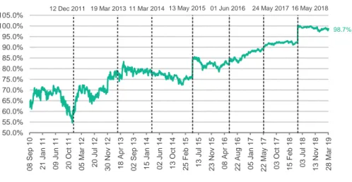
Let us consider the following funding level progression for client XYZ, which proceeds from the data shown in graph 1 of Appendix A, with inception as at 8 September 2010:

16 50.0% 55.0% 60.0% 65.0% 70.0% 75.0% 80.0% 85.0% 90.0% 95.0% 100.0% 105.0% 0 8 S e p 1 0 2 1 Ja n 1 1 0 9 Ju n 1 1 2 0 O ct 1 1 0 5 M a r 1 2 2 0 Ju l 1 2 3 0 No v 1 2 1 8 A p r 1 3 0 2 S e p 1 3 1 5 Ja n 1 4 0 2 Ju n 1 4 1 3 O ct 1 4 2 5 F e b 1 5 1 3 Ju l 1 5 2 3 No v 1 5 0 8 A p r 1 6 2 2 A u g 1 6 0 5 Ja n 1 7 2 2 M a y 1 7 0 3 O ct 1 7 1 5 F e b 1 8 0 3 Ju l 1 8 1 3 No v 1 8 2 8 M a r 1 9

Funding Level Recalibration Date

12 Dec 2011 19 Mar 2013 11 Mar 2014 13 May 2015 01 Jun 2016 24 May 2017 16 May 2018

98.7%

The first thing to note is that we have 8.5 years of investment and overall information, which will give us the opportunity to apply attribution analysis through a broad and continuous range of data. It is the regularity of positive excess returns through overweight positions in over performing sectors (timing) and the right pick of securities that will point towards manager skill or the lack of it.

Secondly, this is an ideal standard scheme and the presence of recalibrations keeps this graph a representative one of real schemes. The jumps usually accompanying recalibrations may have to do with cash inflows made by the client to sustain the scheme’s long-term objectives. Yet, it is not the focus of this study to understand how they are calculated and when they happen.

Finally, this standard scheme has had a growth-matching ratio of 60%/40% at earlier stages and 30%/70% at later stages. This will provide a richer attribution analysis over time. To perform this, we will select 2 dates of analysis: one where more is being allocated to the growth portfolio and another where more is being allocated to the matching portfolio:

Analysis Date Funding Level Growth Allocation

31/12/2014 74.3% 54.2%

31/12/2018 97.9% 31.4%

Figure 1 - Funding Level Progression

17

3.2.2 The portfolio and the benchmark

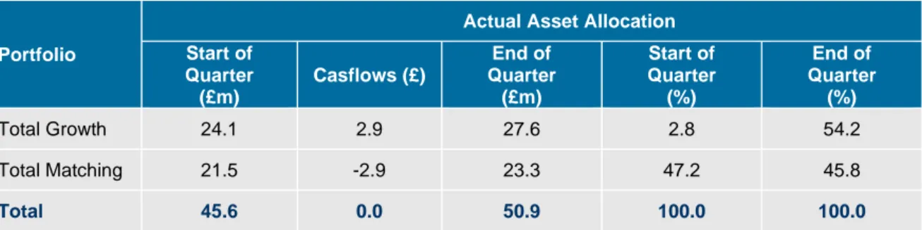
In this section, the focus will be on both portfolios and benchmarks and on assessing manager skill within an equity and bond portfolio environment. Let us consider the following asset allocation as at 31-12-2014.

Portfolio

Actual Asset Allocation Start of Quarter (£m) Casflows (£) End of Quarter (£m) Start of Quarter (%) End of Quarter (%) Total Growth 24.1 2.9 27.6 2.8 54.2 Total Matching 21.5 -2.9 23.3 47.2 45.8 Total 45.6 0.0 50.9 100.0 100.0

We present cashflows for both growth and matching portfolios because we are interested in studying performances in the manager’s point of view. For example, the asset value of the matching portfolio has increased despite of negative cashflows. This means that the portfolio surely had a positive performance over the quarter. On the other hand, the value of the growth portfolio increased by c. £3.5m. However, there were cashflows which would have inflated the value of an MWRR calculated over the same period.

We now present the asset allocation as at 31-12-2018.

Portfolio

Actual Asset Allocation Start of Quarter (£m) Casflows (£) End of Quarter (£m) Start of Quarter (%) End of Quarter (%) Total Growth 21.1 1.6 22.2 29.9 31.4 Total Matching 49.5 -2.2 48.4 70.1 68.6 Total 70.6 -0.6 70.5 100.0 100.0

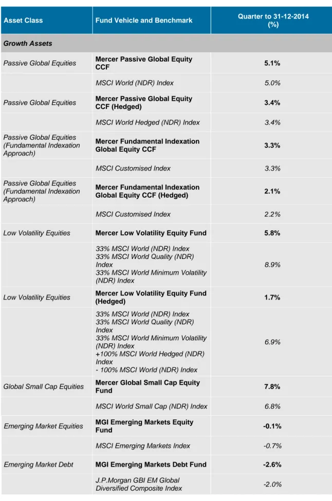
The table below sets out the performance of the assets classes invested as at 31 December 2014. Full actual asset allocations and performance tables for both periods are presented in the appendices B, C and D.

Table 3 – Overview of the portfolio asset allocation as at 31-12-2018 Table 2 – Overview of the portfolio asset allocation as at 31-12-2014

18

Table 4 – Performance by asset class as at 31-12-2014

Asset Class Fund Vehicle and Benchmark Quarter to 31-12-2014 (%)

Growth Assets

Passive Global Equities Mercer Passive Global Equity

CCF 5.1%

MSCI World (NDR) Index 5.0%

Passive Global Equities Mercer Passive Global Equity

CCF (Hedged) 3.4%

MSCI World Hedged (NDR) Index 3.4%

Passive Global Equities (Fundamental Indexation Approach)

Mercer Fundamental Indexation

Global Equity CCF 3.3%

MSCI Customised Index 3.3%

Passive Global Equities (Fundamental Indexation Approach)

Mercer Fundamental Indexation

Global Equity CCF (Hedged) 2.1%

MSCI Customised Index 2.2%

Low Volatility Equities Mercer Low Volatility Equity Fund 5.8%

33% MSCI World (NDR) Index 33% MSCI World Quality (NDR) Index

33% MSCI World Minimum Volatility (NDR) Index

8.9%

Low Volatility Equities Mercer Low Volatility Equity Fund

(Hedged) 1.7%

33% MSCI World (NDR) Index 33% MSCI World Quality (NDR) Index

33% MSCI World Minimum Volatility (NDR) Index

+100% MSCI World Hedged (NDR) Index

- 100% MSCI World (NDR) Index

6.9%

Global Small Cap Equities Mercer Global Small Cap Equity

Fund 7.8%

MSCI World Small Cap (NDR) Index 6.8%

Emerging Market Equities MGI Emerging Markets Equity

Fund -0.1%

MSCI Emerging Markets Index -0.7%

Emerging Market Debt MGI Emerging Markets Debt Fund -2.6%

J.P.Morgan GBI EM Global

19

Performance is in GBP terms using unswung returns for the underlying portfolios.

For benchmark calculation purposes, we have used the following split for the growth portfolio. Multiplying each one of these values by the total growth allocation will generate the weight of the benchmark in each sector (𝑊𝑖):

Asset Class Fund Vehicle and Benchmark Quarter to 31-12-2014 (%)

Multi-Asset Credit Mercer Multi-Asset Credit Fund

(Hedged) -1.1%

50% ICE BofAML Global High Yield Constrained Index, 50% S&P US Leveraged Loans Index

-1.4%

Hedge Funds/Alternatives Mercer Liquid Alternatives

Strategies (Hedged) 2.9%

HFRI FOF: Market Defensive Index 2.9%

HLV Property Mercer High Income UK Property _CCF 1.2%

FTSE A Over 15 Year Gilts Index 11.2%

Matching Assets

Flexible Fixed

Mercer Flexible LDI Fixed Enhanced Hedging Matching Fund

12.9%

Custom Benchmark 12.9%

Long Flexible Fixed Mercer Flexible LDI Fixed

Enhanced Matching Fund 3 26.4%

Custom Benchmark 26.4%

Medium Flexible Real Mercer Flexible LDI Real

Enhanced Matching Fund 2 18.6%

Custom Benchmark 18.6%

Long Flexible Real Mercer Flexible LDI Real

Enhanced Matching Fund 3 22.6%

Custom Benchmark 22.6%

Total Total Scheme 11.7%

20

The benchmark weights for the each of the matching portfolio sectors are drifting with the actual asset values, as mentioned in 2.1.4.

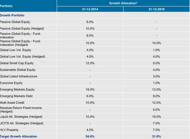
Attribution analysis is useful in studying the sources of excess return compared to a benchmark. Typically, excess return comes from active funds, i.e., funds invested in the growth portfolio, since the aim of active funds is to generate excess return. Matching funds usually aim to cover the gap generated by the increase and decrease in value of liabilities. Therefore, we will focus our analysis on active funds only. The table below shows total growth performances (excluding passive funds) for each period.

3 _{The target growth allocation is usually outlined in a side letter – the Investment Management Agreement}

(IMA). The growth portfolio sub-allocations are reviewed on a timely basis.

Portfolio Growth Allocation

3

31-12-2014 31-12-2018

Growth Portfolio

Passive Global Equity 6.0% -

Passive Global Equity (Hedged) 10.0% -

Passive Global Equity - Fund.

Indexation 6.0% -

Passive Global Equity - Fund.

Indexation (Hedged) 10.0% 10.0%

Global Low Vol. Equity 4.0% 1.0%

Global Low Vol. Equity (Hedged) 4.0% 4.0%

Global Small Cap Equity 12.0% 5.0%

Sustainable Global Equity - 4.0%

Global Listed Infrastructure - 3.0%

Eurozone Equity - 1.0%

Emerging Markets Equity 18.0% 13.0%

Emerging Markets Debt 6.0% 9.0%

Multi-Asset Credit 10.0% 12.0%

Absolute Return Fixed Income

(Hedged) - 5.0%

Liquid Alt. Strategies (Hedged) 10.0% 19.0%

UCITS Alt. Strategies (Hedged) - 7.0%

HLV Property 4.0% 7.0%

Target Growth Allocation 54.0% 31.0% Table 5 – Target growth allocation

21

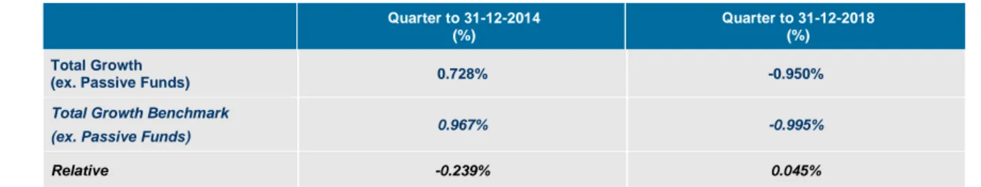
Total Growth

(ex. Passive Funds) 0.728% -0.950%

Total Growth Benchmark

(ex. Passive Funds) 0.967% -0.995%

Relative -0.239% 0.045%

Despite showing a positive performance over the fourth quarter of 2014, the scheme has underperformed its benchmark by 23.9 bps. During the quarter up to December 2018, the scheme has outperformed its benchmark by 4.5 bps, resulting in a negative performance of -0.950%.

Benchmark calculations can be quite demanding and time-consuming. The benchmark of each sector should be adequate (taking into account performance and risk objectives) and it can change over time if another one is more appropriate. As an example, the HFRI FOF: Market Defensive Index (alternative funds’ benchmark) is updated every month. Multi-Asset Credit benchmark has a 1-month lag. Tailored Credit Fund benchmark is given by the return of the fund’s unswung adjusted price gross asset value. Some benchmarks are provided on a daily basis, others on a monthly basis, others on a quarterly basis, which has impact on the calculations.

We have also referred to the concept of rebalancing. In our analysis, we rebalanced the benchmark on a monthly basis and on dates with significant cashflows (established as being greater than 2% of total portfolio). This has to do with the drifts of the matching portfolio. If we had used only one allocation for each fund in the matching portfolio (as at quarter end for example), it would not reflect the portfolio movements along time. So, in a way, more splits is synonym of higher accuracy. Rebalancing becomes essential as more funds drift.

Two questions arise: what are the sources of excess returns? How can we assess the manager’s skill during those periods? One thing is certain: one cannot base our appraisal on just one or two periods of time and expect an accurate description of reality. When monitoring funds performances, it is important to keep historical data to make further analysis.

Quarter to 31-12-2014 (%)

Quarter to 31-12-2018 (%)

22

3.2.3 BHB and BF Models

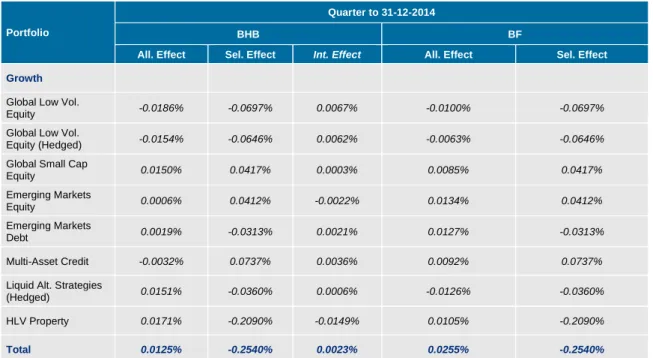
As discussed previously, attribution analysis is a good method to isolate sources of excess return and understand manager skill in making active investment decision. In the table below, we apply both BHB and BF models for the period ending as at 31-12-2014:

We now turn our attention to the two following aspects. The first is that the sum of the effects should be very close (due to rounding) to the excess return. In this example, the BHB proves to be more precise, with a difference of -0.00003%. The BF model shows a difference of c. 0.011%. Secondly, notice that the allocation effects for the Multi-Asset Credit and Liquid Alternatives Strategies funds have opposite signs when comparing both models. Let us consider the case of the Multi-Asset Credit fund. The BHB model states that it had a negative allocation effect on the total excess return because on average the manager had an overweight position in a fund that had a negative performance. The BF model creates a clear contrast by stating that there was a positive allocation effect since the benchmark was overperforming relative to the total growth benchmark, along each sub period. On the other hand, the BHB model states that the Liquid Alternatives Strategies fund was overweighed in a sector that had a positive performance over the quarter. The same analysis of

Portfolio

Quarter to 31-12-2014

BHB BF

All. Effect Sel. Effect Int. Effect All. Effect Sel. Effect

Growth

Global Low Vol.

Equity -0.0186% -0.0697% 0.0067% -0.0100% -0.0697%

Global Low Vol.

Equity (Hedged) -0.0154% -0.0646% 0.0062% -0.0063% -0.0646%

Global Small Cap

Equity 0.0150% 0.0417% 0.0003% 0.0085% 0.0417% Emerging Markets Equity 0.0006% 0.0412% -0.0022% 0.0134% 0.0412% Emerging Markets Debt 0.0019% -0.0313% 0.0021% 0.0127% -0.0313% Multi-Asset Credit -0.0032% 0.0737% 0.0036% 0.0092% 0.0737%

Liquid Alt. Strategies

(Hedged) 0.0151% -0.0360% 0.0006% -0.0126% -0.0360%

HLV Property 0.0171% -0.2090% -0.0149% 0.0105% -0.2090%

Total 0.0125% -0.2540% 0.0023% 0.0255% -0.2540%

23

the BF model would suggest that the manager had an overweighed position in a sector that was underperforming.

In general, the allocation effect had a negative impact on the excess return. In terms of trends, this means that the manager was investing in a bearish market. More specifically, both models agree that the manager had a bad timing when investing in the Global Low Volatility Equities funds.

In terms of selection effect, both use the same method and agree that manager impact was overall negative, i.e., securities picking could have achieved better results. It is important to note that we are referring to “manager impact” since usually managers specialize in a specific sector.

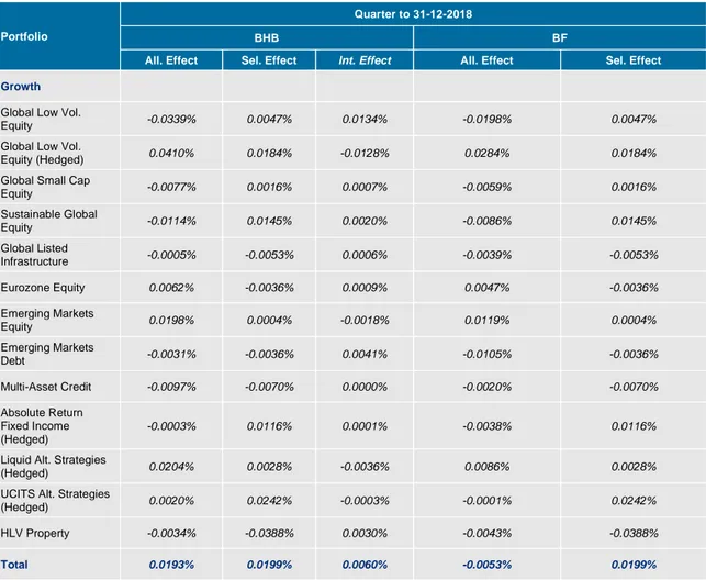
Now, applying the BHB and BF models for the period ending as at 31-12-2018 generates the following figures:

As we are approaching a funding level of 100% (funding level of 97.9% versus 74.3% as at 31-12-2014), more is being allocated to the matching

Portfolio

Quarter to 31-12-2018

BHB BF

All. Effect Sel. Effect Int. Effect All. Effect Sel. Effect

Growth

Global Low Vol.

Equity -0.0339% 0.0047% 0.0134% -0.0198% 0.0047%

Global Low Vol.

Equity (Hedged) 0.0410% 0.0184% -0.0128% 0.0284% 0.0184%

Global Small Cap

Equity -0.0077% 0.0016% 0.0007% -0.0059% 0.0016% Sustainable Global Equity -0.0114% 0.0145% 0.0020% -0.0086% 0.0145% Global Listed Infrastructure -0.0005% -0.0053% 0.0006% -0.0039% -0.0053% Eurozone Equity 0.0062% -0.0036% 0.0009% 0.0047% -0.0036% Emerging Markets Equity 0.0198% 0.0004% -0.0018% 0.0119% 0.0004% Emerging Markets Debt -0.0031% -0.0036% 0.0041% -0.0105% -0.0036% Multi-Asset Credit -0.0097% -0.0070% 0.0000% -0.0020% -0.0070% Absolute Return Fixed Income (Hedged) -0.0003% 0.0116% 0.0001% -0.0038% 0.0116% Liquid Alt. Strategies

(Hedged) 0.0204% 0.0028% -0.0036% 0.0086% 0.0028%

UCITS Alt. Strategies

(Hedged) 0.0020% 0.0242% -0.0003% -0.0001% 0.0242%

HLV Property -0.0034% -0.0388% 0.0030% -0.0043% -0.0388%

Total 0.0193% 0.0199% 0.0060% -0.0053% 0.0199%

24

portfolio (currently 68.6% versus 45.8% as at 31-12-2014), which usually reduces any gap for excess return.

Here again, the BHB proves to be more accurate in summing up all of the effects and match the excess return.

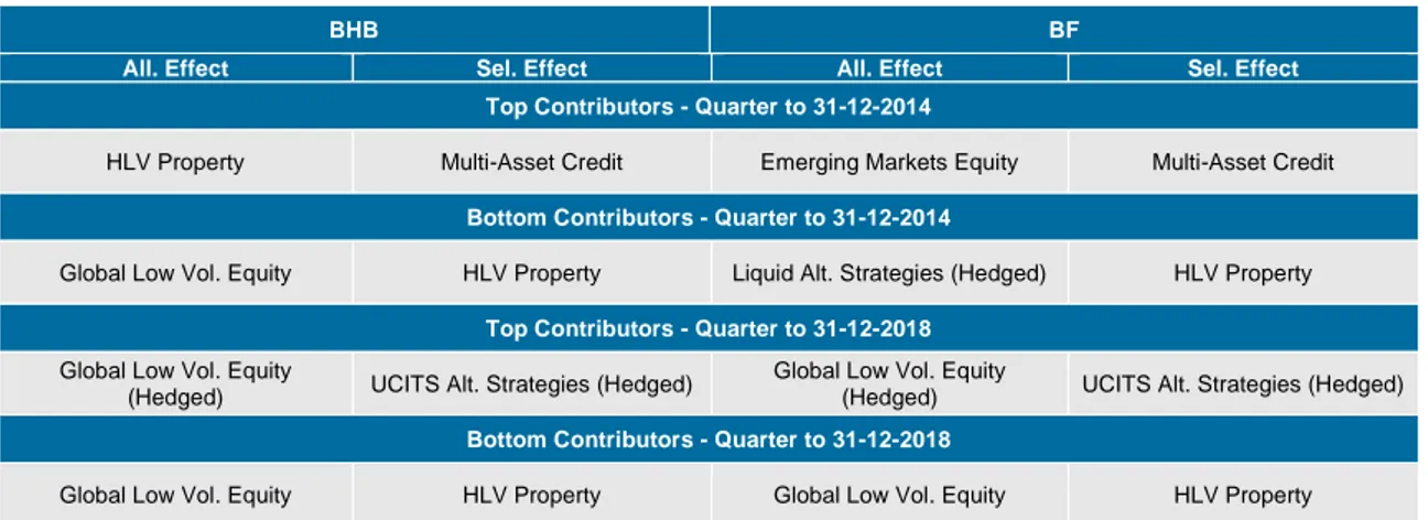
The table below shows the top and bottom contributors (sources) to the excess return of the growth portfolio relative to the growth benchmark (excluding passive funds).

This information tells us about good or bad timing and manager skill in specific periods. However, the repetition of successful investments creates a ranking of managers. The accumulation of these attribution analyses provides us with more information for each period of time and therefore a more accurate way to rank and evaluate managers.

BHB BF

All. Effect Sel. Effect All. Effect Sel. Effect

Top Contributors - Quarter to 31-12-2014

HLV Property Multi-Asset Credit Emerging Markets Equity Multi-Asset Credit Bottom Contributors - Quarter to 31-12-2014

Global Low Vol. Equity HLV Property Liquid Alt. Strategies (Hedged) HLV Property Top Contributors - Quarter to 31-12-2018

Global Low Vol. Equity

(Hedged) UCITS Alt. Strategies (Hedged)

Global Low Vol. Equity

(Hedged) UCITS Alt. Strategies (Hedged) Bottom Contributors - Quarter to 31-12-2018

Global Low Vol. Equity HLV Property Global Low Vol. Equity HLV Property

25

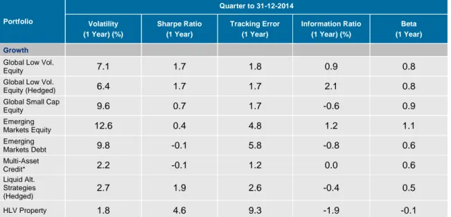
Table 10 – attribution analysis – main risk measures as at 31-12-2014

3.2.4 Risk Attribution Analysis

Active return gives an idea of how successful an investment has been. However, it is also important to take into account the active risk of an investment to understand if the risk taken has paid off. The tables below contain the main risk measures for the active funds of the portfolios and periods under analysis.

*Figures presented are based as of since the inception of the fund: 31-03-2014.

Volatility reflects the total risk of a portfolio. In this case, Global Small Cap and the Emerging Markets Funds pushed the total risk of the portfolio up. This is reasonable for active funds like Emerging Markets Equity, where we can expect strong returns opportunities associated with rapid accentuated growth in specific moments in time. This is also influenced by a beta of c. 1.1, or non-diversifiable risk, which translates how the fund’s performance is affected by variations in the index.

Even though HLV Property significantly underperformed its benchmark, the range of returns over the one-year period has been somehow concentrated. It is interesting to note that beta is the lowest from the funds listed in the table above, accompanying a low volatility of 1.8%. The fund has been able to turn risk into return in an efficient way, as shown by the Sharpe ratio of 4.6.

Now, tracking error is essentially a measure of consistency and describes how well the portfolio is tracking its benchmark, and how much active

Portfolio Quarter to 31-12-2014 Volatility (1 Year) (%) Sharpe Ratio (1 Year) Tracking Error (1 Year) Information Ratio (1 Year) (%) Beta (1 Year) Growth

Global Low Vol.

Equity 7.1 1.7 1.8 0.9 0.8

Global Low Vol.

Equity (Hedged) 6.4 1.7 1.7 2.1 0.8

Global Small Cap

Equity 9.6 0.7 1.7 -0.6 0.9 Emerging Markets Equity 12.6 0.4 4.8 1.2 1.1 Emerging Markets Debt 9.8 -0.1 5.8 -0.8 0.6 Multi-Asset Credit* 2.2 -0.1 1.2 0.0 0.6 Liquid Alt. Strategies (Hedged) 2.7 1.9 2.6 -0.4 0.5 HLV Property 1.8 4.6 9.3 -1.9 -0.1

26

risk has been taken in order to outperform the benchmark. As an example, Global Small Cap Fund was able to outperform its benchmark by c. 1% without taking too much active risk (c. 1.7%). This means that investment decisions played out positively without taking too much active risk. On the other hand, Global Low Volatility Equity Funds and HLV Property show high tracking error values, having significantly underperformed their benchmarks. On a side note, it is common for an active fund to present high tracking error figures, since it aims to maximize excess returns. In the case of passive funds, the goal is to track the benchmark. Consequently, tracking error tends to be smaller.

Information ratio is a way to evaluate a manager’s skill in generating excess return. Similar to the Sharpe ratio, it is a risk-adjusted measure of excess return. It is important to note that one measure is insufficient to make a good portfolio investment analysis. The interpretation of various measures can guide us towards correct conclusions regarding investment decisions. Ideally, an active manager may be looking for a fund with risk characteristics similar to the HLV property above: low volatility, high consistency in generating excess return (high tracking error), low covariance with the market index, for example. The information ratio combined with a high tracking error is a sign that the fund is consistently underperforming its benchmark, and we wish to reach the opposite situation: consistent positive excess returns.

27

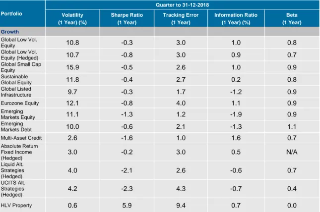
Table 11 – attribution analysis – main risk measures as at 31-12-2018

The fourth quarter of 2018 saw very difficult market conditions, as indicated by a general negative performance by the vast majority of the active funds’ benchmarks. High fluctuations in the risk-free rate increase uncertainty, which translates into higher values of volatility and low Sharpe ratios. Fortunately, the Scheme is now investing more in the Matching portfolio (c. 68.6% of total portfolio valuation). Beta figures above show persistence of non-diversifiable risk over time. Overall, the Total Scheme performed positively, and in line with the benchmark (0.8%).

Despite difficult market conditions, the alternative funds present quite different figures than other funds. This has to do with how those portfolios are built and managers’ investment strategies; however, this is out of the scope of this work and may be topic for another study. Bearing in mind that these measures are based on a one-year series of data, HVL Property has still been successful in generating positive excess return relative to the risk-free rate for each unit of risk. Low volatility combined with stable positive excess return lead to a high tracking error.

Portfolio Quarter to 31-12-2018 Volatility (1 Year) (%) Sharpe Ratio (1 Year) Tracking Error (1 Year) Information Ratio (1 Year) (%) Beta (1 Year) Growth

Global Low Vol.

Equity 10.8 -0.3 3.0 1.0 0.8

Global Low Vol.

Equity (Hedged) 10.7 -0.8 3.0 0.9 0.7

Global Small Cap

Equity 15.9 -0.5 2.6 1.0 0.9 Sustainable Global Equity 11.8 -0.4 2.7 0.2 0.8 Global Listed Infrastructure 9.7 -0.3 1.7 -1.2 0.9 Eurozone Equity 12.1 -0.8 4.0 1.1 0.9 Emerging Markets Equity 11.1 -1.3 1.2 -1.9 0.9 Emerging Markets Debt 10.0 -0.6 2.1 -1.3 1.1 Multi-Asset Credit 2.6 -1.6 1.0 1.6 0.7 Absolute Return Fixed Income (Hedged) 3.0 -0.2 3.0 0.5 N/A Liquid Alt. Strategies (Hedged) 4.0 -2.1 2.6 -0.6 0.7 UCITS Alt. Strategies (Hedged) 4.2 -2.3 4.3 -0.7 0.4 HLV Property 0.6 5.9 9.4 0.7 0.0

28

4. Conclusion

After my first contact with the professional world, I believe it is important to highlight and write down three aspects that have stood out during my internship at Mercer.

First, I have always believed doing an internship would be very beneficial and enrich my understanding of the financial market. A hands-on attitude generates interest in the sense that, while studying theoretical models at university, we as students sometimes fail to realize that those models are actually used in the “real world” and are useful for us to assimilate. That is why it was crucial for me to have that contact.

The second aspect has to do with rigour and capacity to connect the dots. In an organization such as Mercer, every member in the chain of production produces part of the final product that will be delivered to the final client. The bigger picture shows that what we do as individuals is reflected on the final product and directly affects the work of the next person in the chain of production. With greater experience and knowledge comes a deeper capacity to make links and make sense out of numbers. Thus, we learn to become more rigorous.

Thirdly, it is good to know in advance that one has to adapt to the company’s needs. I often found it difficult to see in what way the tasks I was performing would develop my master’s final work. Looking back, I now see that it is the duty of the student to find the right people to talk to, to ask the right questions, to find what can be used to produce the report, and what cannot. In other words, to take ownership.

In the end, I consider I have been successful in fulfilling the three purposes outlined in the introduction of this report by understanding the main tasks that were assigned to me during my internship at Mercer and becoming more familiar with the main performance measures used in performance appraisal through attribution analysis.

29

5. References

• Brinson, Gary P., and Nimrod Fachler, Measuring Non-US Equity Portfolio

Performance, in Journal of Portfolio Management, Spring 1985, pp. 73-76.

• Brinson, Gary P., L. Randolph Hood, and Gilbert L. Beebower, Determinants of

Portfolio Performance, in Financial Analysts Journal, July-August 1986, pp.

39-44.

• Christopherson, Jon A., Ferson, Wayne E., Glassman, Debra A. (1998),

Conditioning Manager Alphas on Economic Information: Another Look at the Persistence of Performance, in The Review of Financial Studies

• Dietz, Peter. O. (1966). Pension funds: measuring investment performance. Free Press

• Elton, J.Edwin, Gruber, J. Martin, Brown, J. Stephen, Goetzmann, N. William, (2017), Modern Portfolio Theory and Investment Analysis, 9th edition, United Kingdom, Wiley Custom

• Fischer, Donald E., Jordan, Ronald J., (1995), Security Analysis and Portfolio

Management, Prentice All, Internacional, Inc.

• Haugen, Robert A., (1997), Modern Investment Theory, 4th _{Edition, International}

Edition

• Sharpe, William F., Alexander, Gordon J., Bailey, Jeffery V., (1999)

Investments, 6th edition, Internation Edition

• Tucker, Alan L., Becker, Kent G., Isimbabi, Michael J., Ogden, Joseph P., (1994), Contemporary Portfolio Theory and Risk Management, West Publishing Company ,San Francisco

30 10 20 30 40 50 60 70 80 90 100 0 8 S e p 1 0 2 1 Ja n 1 1 0 9 Ju n 1 1 2 0 O ct 1 1 0 5 M a r 1 2 2 0 Ju l 1 2 3 0 No v 1 2 1 8 A p r 1 3 0 2 S e p 1 3 1 5 Ja n 1 4 0 2 Ju n 1 4 1 3 O ct 1 4 2 5 F e b 1 5 1 3 Ju l 1 5 2 3 No v 1 5 0 8 A p r 1 6 2 2 A u g 1 6 0 5 Ja n 1 7 2 2 M a y 1 7 0 3 O ct 1 7 1 5 F e b 1 8 0 3 Ju l 1 8 1 3 No v 1 8 2 8 M a r 1 9 £m Assets Liabilities

Appendix A

Appendix B

Asset Class Fund Vehicle

Start of Quarter (€m) Cashflow End of Quarter (€m) Start of Quarter (%) End of Quarter (%) Growth Assets

Passive Global Equities Mercer Passive

Global Equity CCF 1.4 0.3 1.7 5.7 6.1 Passive Global Equities

Mercer Passive Global Equity CCF (Hedged)

2.4 0.3 2.7 9.8 9.7

Passive Global Equities (Fundamental Indexation Approach) Mercer Fundamental Indexation Global Equity CCF 1.3 0.3 1.7 5.6 6.1

Passive Global Equities (Fundamental Indexation Approach) Mercer Fundamental Indexation Global Equity CCF (Hedged) 2.3 0.3 2.7 9.8 9.7

Low Volatility Equities

Mercer Low Volatility Equity Fund

0.9 0.1 1.0 3.6 3.6

Low Volatility Equities

Mercer Low Volatility Equity Fund (Hedged)

0.9 0.1 1.0 3.5 3.6

Global Small Cap Equities

Mercer Global Small Cap Equity Fund

2.9 0.4 3.4 12.0 12.4

Emerging Market Equities

MGI Emerging Markets Equity Fund

4.0 0.9 4.9 16.7 17.6 Table 12 – actual asset allocation of the growth and matching portfolios as at 31-12-2014

31

Numbers above do not reflect any real client (swung) prices. Figures may not sum to total due to rounding.

There is a slight predominance of the Growth portfolio over the Matching portfolio, which is more typical of a client that has not yet reached a funding level close to 100%. There is a higher exposure to equity than to bonds. Therefore, we can assume there will be higher risk than in a situation of higher exposure to equity.

Asset Class Fund Vehicle

Start of Quarter (€m) Cashflow End of Quarter (€m) Start of Quarter (%) End of Quarter (%)

Emerging Market Debt MGI Emerging

Markets Debt Fund 1.6 0.0 1.6 6.5 5.6 Multi-Asset Credit Mercer Multi-Asset Credit Fund (Hedged) 1.9 0.5 2.9 7.8 10.4 Hedge Funds/Alternatives Mercer Liquid Alternatives Strategies (Hedged) 3.0 0.0 3.1 12.4 11.1

HLV Property Mercer High Income

UK Property CCF 1.1 0.0 1.2 4.7 4.2 Cash MGI UK Cash Fund 0.5 -0.5 - 2.0 -

Total Growth Assets 24.1 2.9 27.6 100.0 100.0

Matching Assets

Flexible Fixed

Mercer Flexible LDI Fixed Enhanced Hedging Matching Fund

2.3 -2.0 0.7 10.7 3.1

Long Flexible Fixed

Mercer Flexible LDI Fixed Enhanced Matching Fund 3

1.9 0.7 3.1 8.7 13.5

Medium Flexible Real

Mercer Flexible LDI Real Enhanced Matching Fund 2

5.4 -2.1 4.2 25.0 18.0

Long Flexible Real

Mercer Flexible LDI Real Enhanced Matching Fund 3

11.9 0.5 15.2 55.5 65.4

Total Matching Assets 21.5 -2.8 23.3 100.0 100.0

32

Appendix C

Asset Class Fund Vehicle

Start of Quarter (€m) Cashflow End of Quarter (€m) Start of Quarter (%) End of Quarter (%) Growth Assets

Passive Global Equities (Fundamental Indexation Approach) Mercer Fundamental Indexation Global Equity CCF (Hedged) 2.2 0.4 2.3 10.3 10.2

Low Volatility Equities

Mercer Low Volatility Equity Fund

1.0 -0.7 0.2 4.5 0.9

Low Volatility Equities

Mercer Low Volatility Equity Fund (Hedged)

0.2 0.9 1.0 0.9 4.5

Global Small Cap Equities

Mercer Global Small Cap Equity Fund

1.1 0.2 1.2 5.4 5.3

Sustainable Global Equity Mercer Sustainable

Global Equity Fund 1.0 0.1 1.0 4.5 4.4 Global Listed Infrastructure Mercer Global Listed Infrastructure Fund 0.6 0.0 0.6 2.7 2.6

Eurozone Equity MGI Eurozone

Equity Fund 0.2 0.0 0.2 0.9 0.9

Emerging Market Equities

MGI Emerging Markets Equity Fund

2.7 0.3 2.8 12.7 12.7

Emerging Market Debt MGI Emerging

Markets Debt Fund 1.6 0.4 2.1 7.4 9.4 Multi-Asset Credit

Mercer Multi-Asset Credit Fund (Hedged)

2.8 0.0 2.8 13.3 12.5

Absolute Return Fixed Income Mercer Absolute Return Fixed Income Fund (Hedged) 1.1 -0.1 1.0 5.3 4.7 Hedge Funds/Alternatives Mercer Liquid Alternatives Strategies (Hedged) 3.7 0.0 4.1 17.8 18.5 Hedge Funds/Alternatives Mercer UCITS Alternatives Strategies Fund 1.5 0.0 1.5 7.1 6.6

HLV Property Mercer High Income

UK Property CCF 1.5 0.0 1.5 7.1 6.8

Total Growth Assets 21.1 1.6 22.2 100.0 100.0

33

Appendix D

Asset Class Fund Vehicle and Benchmark Quarter (%)

Passive Glob. Eq. (Fund. Index.)

Mercer Fundamental Indexation

Global Equity CCF (Hedged) -14.9%

MSCI Diversified Multi Factor

Custom (NDR) Hedged Index -14.8%

Low Vol. Eq. Mercer Low Volatility Equity Fund -7.9%

33% MSCI World (NDR) Index 33% MSCI World Quality (NDR) Index

33% MSCI World Minimum Volatility (NDR) Index

-5.1%

Asset Class Fund Vehicle

Start of Quarter (€m) Cashflow End of Quarter (€m) Start of Quarter (%) End of Quarter (%) Matching Assets

UK Credit Mercer UK Credit

Fund 3.7 0.0 3.7 7.6 7.7

UK Long Gilt MGI UK Long Gilt

Fund 3.3 -0.9 2.5 6.7 5.1

Infltation-Linked Bonds MGI UK Inflation

Linked Bond Fund 9.3 -1.4 8.2 18.8 16.9 Inflation Linked LDI

Bonds

Mercer Sterling Inflation Linked LDI Bond Fund

1.0 0.0 1.0 2.0 2.1

Medium Flex. Fixed

Mercer Flexible LDI Fixed Enhanced Matching Fund 2

1.5 0.0 1.6 3.0 3.3

Long Flexible Fixed

Mercer Flexible LDI Fixed Enhanced Matching Fund 3

8.0 0.0 8.4 16.1 17.3

Medium Flexible Real

Mercer Flexible LDI Real Enhanced Matching Fund 2

3.9 0.0 4.2 7.8 8.6

Long Flexible Real

Mercer Flexible LDI Real Enhanced Matching Fund 3

12.2 0.0 12.3 24.7 25.5

Short Flex. Inf.

Mercer Flexible LDI Short Inflation Enhanced Matching Fund 1

2.6 0.0 2.6 5.2 5.3

Tailored Credit Mercer Tailored

Credit Fund 4.0 0.0 3.9 8.1 8.2

Total Matching Assets 49.5 -2.2 48.4 100.0 100.0

Total 70.6 -0.6 70.5 100.0 100.0

34

Asset Class Fund Vehicle and Benchmark Quarter (%)

Low Vol. Eq. Mercer Low Volatility Equity Fund

(Hedged) -10.1%

33% MSCI World (NDR) Index 33% MSCI World Quality (NDR) Index

33% MSCI World Minimum Volatility (NDR) Index

+100% MSCI World Hedged (NDR) Index

- 100% MSCI World (NDR) Index

-11.5%

Glob. Small Cap Eq. Mercer Global Small Cap Equity

Fund -15.7%

MSCI World Small Cap (NDR) Index -15.8%

Sustainable Glob. Eq. Mercer Sustainable Global Equity

Fund -10.2%

MSCI World (NDR) Index -11.3%

Glob. Infra. Eq. Mercer Global Listed

Infrastructure Fund -0.6%

FTSE Global Core Infrastructure

50/50 (NDR) Index -0.3% Eurozone Eq. MGI Eurozone Equity Fund -13.2%

MSCI EMU (NDR) Index -12.1%

Emerging Market Eq. MGI Emerging Markets Equity

Fund -5.9%

MSCI Emerging Markets (NDR)

Index -5.3%

Emerging Market Debt MGI Emerging Markets Debt Fund 4.6%

J.P.Morgan GBI - EM Global

Diversified Index 4.6%

Multi-Asset Credit Mercer Multi-Asset Credit Fund

(Hedged) -3.4%

50% ICE BofAML Global High Yield Constrained Hegded Index 50% S&P/LSTA US Leveraged Loans Hedged Index

-3.8%

Absolute Return Fixed Income

Mercer Absolute Return Fixed

Income Fund (Hedged) 0.6%

FTSE EUR 1 Month Euro Deposit

Index 0.2%

Hedge Funds/Alternatives Mercer Liquid Alternatives

Strategies (Hedged) -2.8%

HFRI FOF: Market Defensive

Hedged Index -2.8%

Hedge Funds/Alternatives Mercer UCITS Alternatives

Strategies (Hedged) -2.1%

FTSE EUR 1 Month Euro Deposit

35

Asset Class Fund Vehicle and Benchmark Quarter (%)

Property Mercer High Income UK Property

CCF 1.4%

FTSE A Over 15 Year Gilts Index 2.6%

UK Credit Mercer UK Credit Fund -0.4%

ICE BofAML Sterling Corporate & Collateralised (ex-Subordinated Financials) Index

-0.4%

UK Long Gilts MGI UK Long Gilt Fund 2.6%

FTSE A Over 15 Year Gilts Index 2.6%

Inf.-Linked Bonds MGI UK Inflation-Linked Bond

Fund 2.0%

FTSE A Over 5 Year Index-Linked

Gilts Index 2.0%

Inf.-Linked LDI Bonds Mercer Sterling Inflation LDI Bond

Fund -0.9%

LGIM Custom Benchmark -0.9%

Medium Flex. Fixed Mercer Flexible LDI Fixed

Enhanced Matching Fund 2 8.2%

BlackRock Flexi Fixed Medium

Index 8.2%

Long Flex. Fixed Mercer Flexible LDI Fixed

Enhanced Matching Fund 3 5.4%

BlackRock Flexi Fixed Long Index 5.4%

Medium Flex. Real Mercer Flexible LDI Real

Enhanced Matching Fund 2 8.2%

BlackRock Flexi Real Medium Index 8.2%

Long Flex. Real Mercer Flexible LDI Real

Enhanced Matching Fund 3 1.1%

BlackRock Flexi Real Long Index 1.1%

Short Flex. Inf. Mercer Flexible LDI Inflation

Enhanced Matching Fund 1 0.2%

Custom Benchmark 0.2%

Tailored Credit Mercer Tailored Credit Fund 1 -0.8%

No Benchmark Assigned -

Total Total Scheme 0.8%