Atmos. Chem. Phys., 16, 15485–15500, 2016 www.atmos-chem-phys.net/16/15485/2016/ doi:10.5194/acp-16-15485-2016
© Author(s) 2016. CC Attribution 3.0 License.
An upper-branch Brewer–Dobson circulation index for
attribution of stratospheric variability and improved ozone
and temperature trend analysis
William T. Ball1,2, Aleš Kuchaˇr3, Eugene V. Rozanov1,2, Johannes Staehelin1, Fiona Tummon1, Anne K. Smith4, Timofei Sukhodolov1,2, Andrea Stenke1, Laura Revell1,5, Ancelin Coulon1, Werner Schmutz2, and Thomas Peter1 1Institute for Atmospheric and Climate Science, Swiss Federal Institute of Technology Zurich, Universitaetstrasse 16, 8092 Zurich, Switzerland
2Physikalisch-Meteorologisches Observatorium Davos World Radiation Centre, Dorfstrasse 33, 7260 Davos Dorf, Switzerland
3Department of Atmospheric Physics, Faculty of Mathematics and Physics, Charles University, V Holesovickach 2, 180 00 Prague 8, Czech Republic
4National Center for Atmospheric Research, Boulder, Colorado 5Bodeker Scientific, Alexandra, New Zealand
Correspondence to:William T. Ball ([email protected])
Received: 25 May 2016 – Published in Atmos. Chem. Phys. Discuss.: 8 July 2016
Revised: 28 November 2016 – Accepted: 28 November 2016 – Published: 15 December 2016
Abstract. We find that wintertime temperature anoma-lies near 4 hPa and 50◦N/S are related, through
dynam-ics, to anomalies in ozone and temperature, particularly in the tropical stratosphere but also throughout the upper stratosphere and mesosphere. These mid-latitude anoma-lies occur on timescales of up to a month, and are related to changes in wave forcing. A change in the meridional Brewer–Dobson circulation extends from the middle strato-sphere into the mesostrato-sphere and forms a temperature-change quadrupole from Equator to pole. We develop a dynami-cal index based on detrended, deseasonalised mid-latitude temperature. When employed in multiple linear regression, this index can account for up to 60 % of the total variabil-ity of temperature, peaking at∼5 hPa and dropping to 0 at ∼50 and∼0.5 hPa, respectively, and increasing again into the mesosphere. Ozone similarly sees up to an additional 50 % of variability accounted for, with a slightly higher max-imum and strong altitude dependence, with zero improve-ment found at 10 hPa. Further, the uncertainty on all equa-torial multiple-linear regression coefficients can be reduced by up to 35 and 20 % in temperature and ozone, respectively, and so this index is an important tool for quantifying current and future ozone recovery.
1 Introduction
Trend analysis, typically using multiple linear regression (MLR), is a key approach to understand drivers of long-term changes in the stratosphere (e.g. WMO, 1994; Soukharev and Hood, 2006; Chiodo et al., 2014; Kuchar et al., 2015; Harris et al., 2015). Ozone and temperature have received most at-tention, partly because they have the longest observational records. Temperature is important for understanding climate change, while quantifying changes in the ozone layer is nec-essary to estimate the impacts of elevated, or reduced, ultra-violet (UV) radiation reaching the surface, especially follow-ing the implementation of the Montreal Protocol to reduce halogen-containing ozone-depleting substances (ODSs).
Ozone and temperature variations in the stratosphere are directly modulated by changes in solar flux, particularly in the UV (see e.g. Haigh et al., 2010; Ball et al., 2016, and references therein). Ozone concentration also responds to changes in the Brewer–Dobson circulation (BDC), whereby air rises in the tropics, advects polewards either on a lower shallow (below∼50 hPa) or an upper deep branch, and de-scends at mid-latitudes (less than∼60◦) or over the poles
waves that break and impart momentum, acting like a paddle to drive the circulation (Haynes et al., 1991; Holton et al., 1995; Butchart, 2014). Wave forcing depends on the mean state of the flow, and vice versa (Charney and Drazin, 1961; Holton and Mass, 1976); changes in either affect ozone trans-port by a change in the speed of the BDC that leads to adiabatic heating, or cooling, and directly affects chemistry through temperature-dependent reaction rates (Chen et al., 2003; García-Herrera et al., 2006; Shepherd et al., 2007; Lima et al., 2012). As such, ozone and temperature have an inverse relationship in the equatorial stratosphere above 10 hPa, which in turn has a dependence on dynamics (Fusco and Salby, 1999; Mäder et al., 2007; Stolarski et al., 2012), although this is not always the case in the lower stratosphere (Zubov et al., 2013). Ultimately, then, dynamical perturba-tions at mid-to-high latitudes can directly influence the vari-ability of ozone and temperature (Sridharan et al., 2012; Nath and Sridharan, 2015).
The stratospheric ozone layer has been damaged by the use of ODSs, and, following a ban through the 1987 Mon-treal Protocol (Solomon, 1999), levels of ODSs have de-clined since their peak in 1998 (Egorova et al., 2013; Chip-perfield et al., 2015), although the peak may be earlier or later depending on the location of interest. However, the rate of ozone recovery is latitude dependent, with southern mid-to-high latitudes expected to recover from elevated ODSs (WMO, 2011). The increase in ozone at mid-latitudes comes partly from ODS reductions but is also because the BDC is expected to accelerate (Garcia and Randel, 2008; Butchart and Scaife, 2001; Butchart, 2014), which will reduce the time for ozone depletion to occur and lead to faster transport of ozone from the equatorial region to higher latitudes. This in turn leads to a reduction of ozone over the Equator and a pre-vention of a full recovery over the tropics. Thus, the recovery of ozone at mid-to-high latitudes can be understood as being partly due to less ozone destruction by lower ODS concen-trations and partly due to a faster redistribution of ozone-rich air from the tropics. Additionally, the cooling stratosphere will slow ozone depletion and further support the increase in ozone at mid-latitudes (WMO, 2014). However, estimates of decadal trends in ozone since 1998 have a high level of uncer-tainty (Harris et al., 2015) because various long-term datasets provide different pictures (Tummon et al., 2015), and we do not understand much of the stratospheric variability on short timescales. Anomalous monthly variability, like that at the Equator as shown in Figs. 7 and 8 in Shapiro et al. (2013), and which could be related to high-latitude variability (e.g. Kuroda and Kodera, 2001; Hitchcock et al., 2013), may sim-ply be considered as noise in MLR trend estimates (and other regressors) where it is not accounted for, which increases the uncertainty.
In MLR analysis of the equatorial stratosphere, variability is usually described with at least six regressors that repre-sent the solar cycle UV flux changes (e.g. with the F10.7 cm radio flux); volcanic eruptions (stratospheric aerosol optical
depth: SAOD); the El Niño Southern Oscillation (ENSO) surface temperature variations; two orthogonal modes of the dynamical quasi-biennial oscillation (QBO); and the equiva-lent effective stratospheric chlorine (EESC), which describes the long-term influence of ODSs on ozone concentration and temperature. A greenhouse gas (GHG) proxy is sometimes also considered, or, alternatively to applying both GHG and EESC proxies, a linear (or piece-wise linear) trend is consid-ered.
At higher latitudes, other proxies have been used to rep-resent dynamical indices, e.g. in the Northern Hemisphere (NH), the North Atlantic Oscillation (NAO) and Arctic Os-cillation (AO), which are related to surface pressure changes, though their relation is less anti-correlated with stratospheric variability than, e.g., the tropopause pressure (Weiss et al., 2001). Trends in dynamically related quantities, such as horizontal advection and mass divergence, contribute to long-term changes in ozone (Wohltmann et al., 2007). For short timescales, Wohltmann et al. (2007) note that tropo-spheric pressure is a physical quantity directly responsible for changes in lower-stratospheric temperatures but that it is nevertheless inferior to stratospheric temperature when accounting for ozone and temperature variance in column ozone and temperature; this can also depend on the loca-tion of tropospheric blocking events (WMO, 2014). How-ever, longer timescales render these proxies unreliable due to additional radiative effects. Ziemke et al. (1997) identi-fied that the use of high-latitude temperature at 10 hPa in winter–spring months, together with 200 hPa temperature at mid-latitudes all year round, was most effective at reducing residuals, though Ziemke et al. (1997) limited their study to total column ozone.
In fact, several studies have identified proxies, such as temperature in the stratosphere, that can help improve MLR analysis (e.g. Ziemke et al., 1997; Appenzeller et al., 2000; Weiss et al., 2001; Mäder et al., 2007). However, these have tended to be focused on total column ozone, the mid-to-lower stratosphere, or mid-latitude and polar regions, and thus most attention on dynamical variability remains associ-ated with the lower branch of the BDC (e.g. Newman et al., 2001; Wohltmann et al., 2005; Brunner et al., 2006). Further, studies of dynamical variability have also tended to focus on seasonal and inter-annual timescales, and thus any fluctua-tions on monthly or shorter timescales may be missed, un-derestimated, or driven by processes operating on different timescales.
W. T. Ball et al.: Upper-stratosphere dynamics index 15487 variables – that go unnoticed because error statistics do not
change or, indeed, decrease. A third approach simply con-siders dynamical variability as noise that leads to enhanced uncertainties on trend analysis.
The identification of a correlation between two variables can be considered a first step in identifying the physical mechanism that underlies the causal link. A relationship be-tween the proxies and processes that drive their variability needs to be shown through additional information; it cannot be done simply through statistical means alone as it needs information from a physical understanding, either a priori or following further investigation. Here, our aim is to find an in-dex, or proxy, that represents rapid changes, on timescales of a month or less, in the upper branch of the BDC by investigat-ing an identified association between temperature variation in the mid-latitude upper stratosphere and planetary wave breaking. While temperature alone does not represent a com-plete picture of the physical driver of rapid BDC changes, we show that its variance is highly associated with wave driv-ing and that it can act as a proxy for such processes, espe-cially where the exact physical drivers remain unresolved; the use of standard dynamical proxies is, as we shall show, not enough to capture this variance. Chandra (1986) identi-fied similar short-term dynamical variability that we identify in monthly data here, but he applied it to understand dynam-ical influences on upper-stratospheric variability relevant to identifying 27-day solar irradiance variability – indeed show-ing that 27-day solar modulation was very difficult to identify due to large, rapid dynamical fluctuations – and did not ex-trapolate this information to improving MLR analysis, as we aim to do here. The drawback to using temperature is that it mixes processes that might have different influences on ozone (Wohltmann et al., 2005). However, it is a simple and direct measure of dynamical changes, at least on monthly or shorter timescales, that relate to rapid dynamical adjustments within the stratosphere.
In summary, our aim here is to provide an index (Sect. 4) to account for sporadic, noise-like stratospheric variability in monthly time series that represents rapid adjustments in the BDC and, therefore, better account for residual variance, improve estimates of trends and regressor variability, and duce their uncertainties (Sect. 5). We do this using model, re-analysis, and observational data (Sect. 2) to identify a source for the short-term variability (Sect. 3).
2 Data and models
2.1 Chemistry–climate model in specified-dynamics mode
To investigate temperature and ozone variability in the strato-sphere and mesostrato-sphere at all latitudes, without data gaps, we simulate historical ozone and temperature variations using the chemistry–climate model (CCM) SOlar Climate Ozone
Links (SOCOL, version 3; Stenke et al., 2013) in specified-dynamics mode, whereby the vorticity and divergence of the wind fields and temperature, and the logarithm of sur-face pressure are “nudged” using the ERA-Interim reanalysis (Dee et al., 2011) between 1983 and 2012 and up to 0.01 hPa; see Ball et al. (2016) for full nudging details. Note that we use the Stratospheric–tropospheric Processes And their Role in Climate (SPARC)/International Global Atmospheric Chemistry (IGAC) Chemistry–Climate Model Intercompari-son (CCMI) boundary conditions and external forcings (Rev-ell et al., 2015), except for the solar irradiance input, for which we use the Spectral And Total Irradiance REconstruc-tion – Satellite era (SATIRE-S) model (Krivova et al., 2003; Yeo et al., 2014). In the following we focus on temperature and ozone variables; the former is nudged, while the latter is simulated by the CCM SOCOL.
2.2 Observations
We verify that the nudged-model output fields ozone (not nudged) and temperature (nudged) agree with observations. For ozone we use the Stratospheric Water and OzOne Satel-lite Homogenized (SWOOSH) ozone composite (Davis et al., 2016) for 215–0.2 hPa (∼10–55 km) at all latitudes. For temperature, we compare the nudged-model output with in-dependent measurements from the Sounding of the Atmo-sphere using Broadband Emission Radiometry (SABER) in-strument (Russell et al., 1999) on the Thermosphere, Iono-sphere, MesoIono-sphere, Energetics, and Dynamics (TIMED) satellite, spanning 2002–2015 and for 100 to 0.00001 hPa (∼10–140 km) and latitudes out to 52◦.
For the MLR analysis (Sect. 5) we additionally consider equatorial ozone from the Global OZone Chemistry And Related trace gas Data records for the Stratosphere (GOZ-CARDS; Froidevaux et al., 2015), Solar Backscatter Ultra-violet Instrument Merged Cohesive (SBUV-Mer.; Tummon et al., 2015), SBUV Merged Ozone Dataset (SBUV-MOD; Frith et al., 2014) composites and temperature from the Stratospheric Sounding Unit observations (SSU; Zou et al., 2014), and Japanese 55-year Reanalysis (JRA-55) (Ebita et al., 2011) and Modern-Era Retrospective analysis for Re-search and Applications (MERRA) (Rienecker et al., 2011) reanalyses. All observations are re-gridded onto the SOCOL model pressure levels and latitudes. We consider monthly mean zonally averaged data.
3 Anomalous dynamical variability
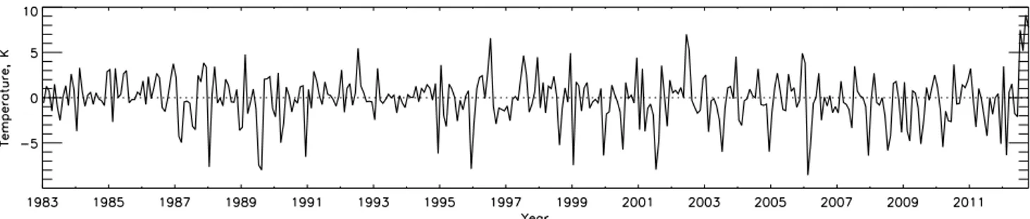
a 13-month running mean, and then deseasonalised, with monthly values, at each latitude and pressure. We apply this pre-processing to all variables described in Sects. 3 and 4. An example equatorial (20◦S–20◦N) ozone and temperature anomaly time series from the CCM SOCOL at 2.5 hPa is shown in Fig. 1. SWOOSH ozone from 1985 to 2012 and SABER temperature from 2002 to 2012 (Fig. 1) show simi-lar anomalies to the model and have correlation coefficients (rc) of 0.72 and 0.83 with the nudged-model results, respec-tively; the model, therefore, reproduces observations well. The monthly temperature and ozone anomalies have a very strong relationship, especially between 0.1 and 6.3 hPa, with negativercreaching−0.96 (Fig. 2) between 0.1 and 10 hPa, while being positive elsewhere.
To establish the coherency of the ozone–temperature re-lationship in the tropics, we identify “extreme” anomalies (or “events”) as those at least at the 90th percentile from the mean in temperature and at less than the 10th percentile for ozone (and vice versa). We call “low-T” events those that have low equatorial temperature at the same time as a high ozone concentration (blue lines at 2.5 hPa, Fig. 2), and “high T” for the opposite situation (red lines); the low-T thresholds are−1.3 K for temperature and+2.4 % for ozone, while high-T thresholds are+1.1 K and−2.2 % (these are also given the upper plot of Fig. 1). We note that the ozone mixing ratio maximum in parts per million (ppm) is at ∼10 hPa. We use 2.5 hPa as a reference here, but other pres-sure levels at altitudes between 0.1 and 6 hPa give similar re-sults. The majority of the events (45/60) occur in December– January–February (DJF; red/blue in Fig. 2) and June–July– August (JJA) (yellow/turquoise in Fig. 2). High-T and low-T months remain grouped above 10 hPa but mix and lose coher-ence at altitudes below 10 hPa, implying that the events have a similar source at all altitudes above 10 hPa but a different one below (i.e. rc is high at 25 and 40 hPa, but the events at 25 hPa are well mixed). This indicates a likely transition between BDC branches and that the driver of variability is dynamical, which we confirm in the following.
3.2 Mid-latitude temperature variability
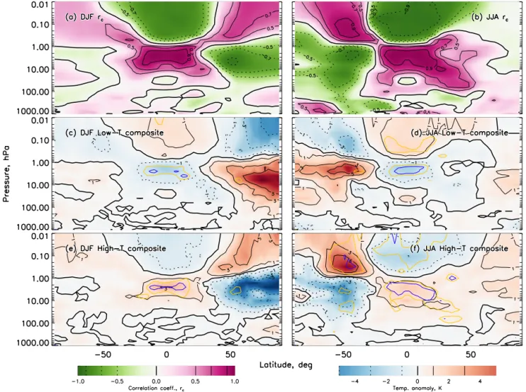
To identify and locate the source of the driver behind ozone and temperature anomalies shown and described in the pre-vious section, in Fig. 3 we correlate the 2.5 hPa equatorial temperature low-T and high-T events with detrended and de-seasonalised temperature at all latitudes and pressure levels, for DJF and JJA months (Figs. 3a and b, respectively). A quadrupole-like structure emerges with positive correlations centred around 2.5 hPa at the Equator and in the winter-polar mesosphere (<0.8 hPa), and negative correlations in the win-ter stratosphere at mid-to-high latitudes and in the equatorial mesosphere. The inverse correlation in the stratosphere for DJF extreme months peaks at ∼52◦N (r
c= −0.92), while JJA events peak at∼43◦S (r
c= −0.93). We find similar
re-sults when using other equatorial pressure levels near 2.5 hPa as a reference to calculate correlations.
Figures 3c–f show temperature composites for each event type: Fig. 3c for DJF lowT, 3d for JJA lowT, 3e for DJF highT, and 3f for JJA highT; all show the same temperature-quadrupole structure as in Fig. 3a–b (signals at 2 and 3 stan-dard deviations from 0 are given as yellow and blue contours, respectively). Equatorial temperature anomalies (∼2 K) are smaller than at high latitudes (∼5 K or more). The maxi-mum temperature response at mid-to-high latitudes does not always reside at the same location as the peak correlation. Although the statistics are less robust, since the period is shorter, the quadrupole structure is also evident in SABER observations (Fig. 4). Thus, we can be confident that the nudged model is giving a good representation of observa-tions.
The quadrupole structure is likely the result of (i) an ac-celeration of the BDC that adiabatically cools the Equator during low-T events as more air arrives at high latitudes and adiabatically heats there, and (ii) a deceleration of the BDC that adiabatically heats the Equator during high-T events as less air arrives at high latitudes, leading to cooling there; both processes are associated with changes in wave activity.
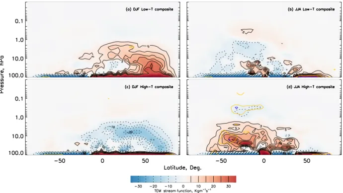
We show that the mid-latitude temperature, the equatorial temperature, and ozone anomalies are related to variations in wave activity using the transformed Eulerian mean stream function (TEMS; Fig. 5), a measure of the mass flux (pos-itive values imply clockwise flow along contours, and neg-ative values anti-clockwise) and the Eliassen–Palm flux di-vergence (EPFD; Fig. 6), which is a measure of the resolved wave-induced forcing of the mean flow (positive values im-ply an acceleration of the zonal-mean flow and a deceleration of the BDC, and negative values the opposite). We used 6-hourly model output to calculate the monthly means and use Eqs. (3.5.1) and (3.5.3) from Andrews et al. (1987) to per-form the calculations. Using the events identified in Figs. 1 and 2, and used in Fig. 3, we find clear EPFD and TEMS anomalies centred near 55◦, slightly poleward of the
there-W. T. Ball et al.: Upper-stratosphere dynamics index 15489
Figure 1.Monthly anomalies of equatorial (20◦S–20◦N) ozone (upper; %) and temperature (lower; degrees Kelvin) at 2.5 hPa, following the subtraction of 13-month box-car smoothing and monthly deseasonalising from the CCM SOCOL model in specified-dynamics mode. SWOOSH ozone composite time series and SABER temperature measurements are shown in light blue in the upper and lower plots, respec-tively. The dashed blue and red horizontal lines are the thresholds shown in Fig. 2; thresholds for each coloured diamond are given in the right of the upper panel. June–July–August (JJA) anomalies exceeding the thresholds have orange (highT) and turquoise (lowT) diamonds; December–January–February (DJF) anomalies are identified by red (highT) and blue (lowT) diamonds.
Figure 2.Regression of equatorial (20◦N–20◦S) ozone and temperature anomalies (following 13-month smoothing and monthly deseason-alising) from the CCM SOCOL model in specified-dynamics mode for pressure levels 0.01 to 40 hPa (∼80–22 km). Grey crosses are for all other months in January 1983–October 2012. Coloured crosses in each plot are determined at 2.5 hPa (lower left, and plotted as diamonds in Fig. 1) by those within regions defined by the red (high-T events) and blue lines (low-T events); red crosses are for high-T events in December, January, and February (DJF); yellow are for high-T events in June, July, and August (JJA); and green are for “other” high-T events. Dark blue, turquoise, and blue represent DJF, JJA, and “other” low-T months, respectively (see also legends in 1.0 and 1.6 hPa plots). Correlation coefficients are given for all crosses together. The yscale has been decreased by a factor of 30 and 5 at 0.01 and 0.05 hPa, respectively, as indicated in the plots.
fore a decrease of ozone, and vice versa for temperature de-creases, though these effects seem to be less important than the rapid profile adjustment itself.
4 Upper-branch Brewer–Dobson circulation (UBDC) index
Figure 3.Correlation coefficient maps of zonal-mean 20◦N–20◦S 2.5 hPa temperature anomalies from the SOCOL model with respect to latitude and altitude for all identified low- and high-T (a)DJF and(b)JJA events, as defined in Fig. 2. (c–f) Composite temperatures for(c) DJF low-T,(d)JJA low-T,(e)DJF high-T, and(f)JJA high-T events. Dashed (solid) contours are negative (positive), with the bold line representing 0. Signals at the 2 and 3 standard deviations from 0 are given as yellow and blue contours, respectively, in(c)–(f).
W. T. Ball et al.: Upper-stratosphere dynamics index 15491
Figure 5.The median of the transformed Eulerian mean stream function (TEMS) anomalies for(a)DJF low-temperature events,(b)JJA low-T events,(c)DJF high-T events,(d)JJA high-T events for the same months as in Fig. 3c–f. Contours lines (solid: positive; dashed: negative) and colours are given in the legend. Positive values indicate clockwise acceleration along the contour lines; negative are anti-clockwise. Data are from the SOCOL model in specified-dynamics mode.
a large proportion of variability previously unaccounted for and drive down uncertainties on regressor estimates. We fo-cus here on the equatorial region, but our results imply this index could be applied to other locations in the stratosphere and mesosphere.
Below, we describe how we construct an UBDC index based on detrended and deseasonalised temperature averaged over 43–49◦S and 2.5–6.3 hPa for June–October, and aver-aged over 52–57◦N and 4–10 hPa for November–May. Our index utilises the output from the CCM SOCOL in specified-dynamics mode, similar to ERA-Interim and observations, but such an index could be constructed in a similar way for any specific model.
4.1 Construction
Constructing a useful UBDC index requires the identification of maximum correlation between the Equator and each hemi-sphere separately, followed by a combination of information from these two regions. We have previously considered just the extreme events, but we now consider all monthly anoma-lies between 1983 and 2012. While wave activity drives the temperature changes, it is not an easily observable quantity. Thus, temperature is a natural and simple quantity to build the index with. Additionally, we have found that the CCM SOCOL in free-running mode (i.e. without nudging) shows the same anomalous temperature-quadrupole structure as in
Fig. 3 (not shown). Therefore, one can easily construct an index using model data to represent anomalous behaviour in the equatorial regions, and elsewhere where there is a quadrupole response.
We identify the maximum inverse temperature correlations at mid-latitudes in both DJF and JJA by varying the reference equatorial pressure level. We find that averaging over the nine grid cells centred on the mid-latitude peak improves the relationship with the equatorial region. Therefore, we con-struct the index with anomalous temperatures averaged over 43–49◦S and 2.5–6.3 hPa in the Southern Hemisphere (SH)
based on JJA months, and 52–57◦N and 4–10 hPa in the NH
based on DJF months.
identi-Figure 6.As for Fig. 5 but for EPFD. Negative values indicate increased wave activity, and positive values decreased activity.
Figure 7.The UBDC index from the CCM SOCOL model in specified-dynamics mode using ERA-Interim from 1983 to 2012.
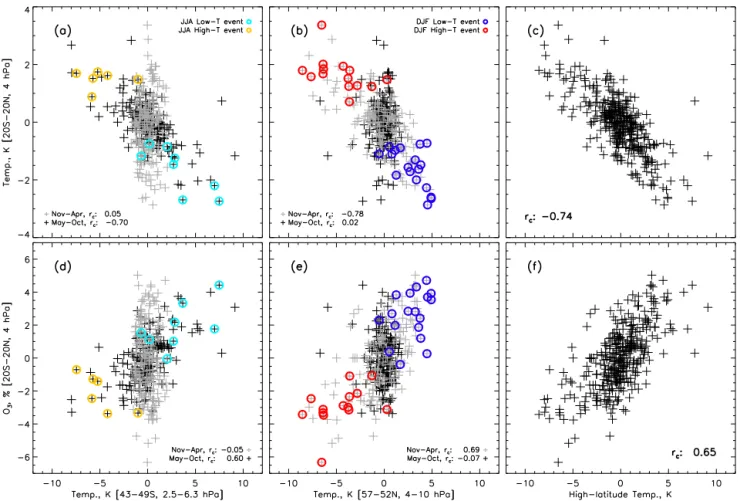
fied in Fig. 1 are highlighted with coloured circles, showing that the equatorial anomalies are related to mid-latitude wave driving. Figure 8c shows the UBDC index plotted against all equatorial temperature anomalies at 4 hPa (rc= −0.74). The lower panels (Fig. 8d–f) show the equatorial ozone re-lationship with respect to mid-latitude temperature and the UBDC index; the absolute correlation coefficient is lower (rc=0.65) than for equatorial temperature in the upper pan-els, but there is still a strong relationship.
In Fig. 9 we show the amount of variability the UBDC in-dex can account for in nudged-model temperature anomalies everywhere (1983–2012), using the coefficient of determina-tionrc2, orR2. It ranges from 0 to 1; a value of 1 is synony-mous with the index accounting for 100 % of the variability. In Fig. 9a the UBDC index can account for >50 % of ability between 10 and 1 hPa, and above 0.05 hPa. The
vari-ability accounted for at mid-latitudes is less (up to∼30 %), even at the index source locations (white circles), because the UBDC index has almost zero agreement half of the time there (see Fig. 8). In Fig. 9b and c, the UBDC index accounts for much of the DJF/JJA variability: above 20 hPa it can ac-count for over 70 % of equatorial variability, more than 60 % of polar mesospheric variability (80 % in the SH), and much of polar stratosphere variability.
W. T. Ball et al.: Upper-stratosphere dynamics index 15493
Figure 8. (a–b)SOCOL equatorial temperature anomalies (4hPa, 20◦N–20◦S) plotted against(a)temperature means from 2.5–6.3 hPa and 43–49◦S and(b)52–57◦N and 4–10 hPa.(d–e)As for upper panels, but equatorial ozone anomalies (4 hPa, 20◦N–20◦S) are instead plotted against high-latitude temperature anomalies. Grey crosses are for November–April months; black crosses for May–October; correlations for both periods are given in each panel. Red and blue circles identify the DJF high-T and low-T events in Figs. 1 and 2, respectively; orange and light-blue circles similarly identify JJA events.(c, f)May–October 43–49◦S temperatures and November–April 52–57◦N temperatures are combined in the right panel (UBDC index) and plotted against equatorial(c)temperature and(f)ozone.
60–90◦S, 60–90◦N, 45–75◦N, and 45–75◦S. We consider
DJF and November–April periods for the Northern sphere, and JJA and May–October for the Southern Hemi-sphere. We considered the original time series, and detrended and deseasonalised versions following the method outlined in Sect. 3.1. We correlated these 32 “proxy” time series with the UBDC index, which we have now shown to have high agree-ment with short-term variability in the upper stratosphere and mesosphere. Considering just the R2values (i.e. coefficient of determination), we found values exceeding 0.15 only for the 100 hPa heat flux in three cases: DJF 60–90◦N after
de-seasonalising and detrending the data, and 0.18 and 0.19 for DJF 45–75◦N, respectively with or without deseasonalising
and detrending; we also found that the third case here has a similar value with a 1-month lag. Results for proxies in the Southern Hemisphere all had values close to 0. While these results suggest there is some possible relationship between the 100 hPa heat flux and dynamical variability in the upper stratosphere, and we concede that this was a simplistic set of
tests, the implication is that very little of the variance we see in temperature above 10 hPa is accounted for by these prox-ies for stratospheric dynamics at lower altitudes. The source of the upper-stratosphere and mesospheric variance warrants further investigation beyond this publication, as our analysis clearly shows a relationship with changes in temperature in the upper stratosphere and mesosphere related to what ap-pears to be a wave-forcing-like response in the EPFD and stream functions (i.e. Figs. 5 and 6).
5 Improvement in MLR analysis using the UBDC index
The UBDC index leads to a large uncertainty reduction in MLR analysis. To show this, we consider MLR with or without the index focused on the equatorial region (20◦S–
20◦N). In both cases we use the two QBO indices, SAOD,
Figure 9. Coefficient of determination (R2) maps of the upper-branch Brewer–Dobson circulation (UBDC) index with SOCOL model temperature at all latitudes and altitudes for(a)all months,(b)DJF, and(c)JJA. White circles represent the approximate region that the UBDC index is derived from.
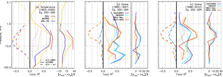
Figure 10.Coefficient of determination summed over all regressors (Rc2) and the reduction in the Student’sttest-based error on regressor coefficients (%) for equatorial profiles (positive values) for(a)temperature from 1983 to 2005, for ozone between(b)1985 and 1997, and for ozone between(c)1998 and 2012 for various datasets (see legends). ForR2, dotted lines represent estimates without the UBDC index, solid lines with, and the difference (without UBDC minus with UBDC) is given as negative and dashed lines.
radio flux as a proxy for solar variability, as this is supe-rior to the F10.7 cm radio flux (Dudok de Wit et al., 2014). We consider the use of “AR2” auto-regressive modelling through the procedure of Cochrane and Orcutt (1949) in all cases; see Tiao et al. (1990) for a discussion of AR. The use of second-order auto-regression was determined after as-sessing the regression analysis using a Durbin–Watson test, which showed that AR1 was necessary but not sufficient to account for auto-correlation in the residuals and that AR2 was sufficient. In Fig. 10a, we show the combined ability of the regression model to account for variance, i.e. the to-talR2of all regressors, for 1983–2005 in SSU temperature observations (red), and JRA-55 (blue) and MERRA (yel-low) reanalyses.R2without the UBDC index (dotted lines; Fig. 10a) shows that only up to∼45 % (R2=0.45) of the stratospheric variability above 10 hPa can be accounted for. However, with the UBDC index (solid lines) R2 is >0.8
(MERRA∼0.7), and, in all cases, the use of the UBDC in-dex peaks at∼5 hPa, with R2increasing by 0.45–0.60, or an improvement of up to 60 % (see negative values in the left panel of Fig. 10a, i.e.R2w/oUBDC-Rw/2 UBDC). In the right panel of Fig. 10a, we show the relative change in regres-sor uncertainty
(σw/o UBDC2 −σw/ UBDC2 )/σw/o UBDC2 ×100
, whereσ is based on Student’st test. The uncertainty esti-mates on the regressors decrease by up to∼35 (SSU),∼35 (JRA-55), and∼10 % (MERRA). In addition, the index in-creasesR2above 0.4 hPa in the mesosphere.
W. T. Ball et al.: Upper-stratosphere dynamics index 15495
(a) (b) (c)
Figure 11.The full distributions ofR2from MLR of SSU equatorial temperature (20◦S–20◦N, 1983–2005) without (w/o, blue) and with (w, red) the UBDC index showing(a)4.6 hPaR2values for all the regressors considered in the analysis, as well as the total;(b)the annual and seasonal totalR2at 4.6 hPa; and(c)the annual totalR2for the three SSU pressure levels. Distributions were calculated from 10 000 bootstrapped samples for each of the possible (n=6) 720, or (n=7) 5040, order of regressors. Solid white lines are the median values; dotted lines are the 68 % confidence intervals.
case for the 3 decades we consider here (see e.g. Chiodo et al., 2014). We use the robust Lindeman–Gold–Merenda (LGM) measure (Lindeman et al., 1980), which determines relative importance by averaging over all possible,n!, order-ing of regressors (720 for six regressors, 5040 for seven). In Fig. 11a we show the relative importance of each regres-sor, as well as the total, in representing the variance in SSU temperature at 4.6 hPa; curves represent the complete dis-tributions resulting from 10 000 bootstrappings of averages over orderings. At 4.6 hPa the UBDC index accounts for ∼61 % of temperature variance when considered in addition to the others, partly at the expense of decreasing the rela-tive importance of the other regressors. Together, the UBDC leads to a ∼44 % increase in the total variance accounted for, from 38 to 82 % (peak values: solid white lines); we see similar results at the other two pressure levels (Fig. 11c). Figure 11b shows that seasonal MLR analysis is enhanced: March–April–May (MAM), JJA, and DJF peaks increase by more than double the 68 % confidence intervals, i.e. by an additional∼22,∼40, and∼33 %, respectively; September– October–November (SON) months do not improve much (∼10 %).
Similar results are found for ozone. Figure 10b and c show the ozone composites (see Sect. 2.2) split into 1985–1997 and 1998–2012 time periods, reflecting those often used to investigate ozone trends (e.g. Harris et al., 2015). There are significant differences in R2between the ozone composites from the MLR analysis, which reflects the fact that
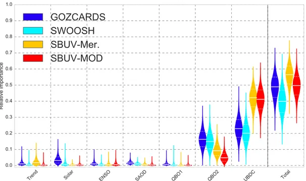
Figure 12.Similar in format and method to Fig. 11a, the relative importance of each regressor using the coefficient of determination (R2), as well as the combined total, is shown from multiple linear regression analysis of four ozone composite datasets at 1.6 hPa for 20◦S–20◦N and 1998–2012. The most-likely value is given by the central, solid white line, and the dotted lines are the 68 % confidence intervals. Distributions were calculated from 10 000 bootstrapped samples of each of the possible 5040 regressor orderings.
Figure 13.Equatorial stratospheric decadal trend profiles for (left) SWOOSH (light blue), GOZCARDS (blue), SBUV-Mer. (yellow), and SBUV-MOD (red) ozone between 1998 and 2012, and (right) for SSU (red), MERRA (yellow), and JRA-55 (blue) temperature between 1983 and 2005. Thin lines and circles represent profiles without the UBDC index; thick lines and filled circles are with the UBDC index. The change in error bars are the same reduction in the error bar between using and not using the UBDC index as in Fig. 10. Profiles have been offset slightly from the actual pressure levels for clarity.
We note that the UBDC index influences the relative im-portance of most of the other regressors by less than the 68 % confidence interval (dashed white lines in Fig. 12), and only in the case of the trend does the relative importance get de-creased by a larger margin, albeit within 95 %. Figure 13b shows that the mean values of the SSU MLR results are
W. T. Ball et al.: Upper-stratosphere dynamics index 15497 the same way as temperature (not shown), so the larger effect
on the SSU relative importance may be data dependent. In Fig. 13 we show the equatorial decadal trend profiles of the datasets considered in Fig. 10 and the 2σ uncertain-ties derived from multiple linear regression with (thick lines) and without (thin lines) the UBDC index, between 25 and 0.2 hPa. A full discussion of the differences in the ozone pro-files is undertaken by Tummon et al. (2015) and Harris et al. (2015), so we do not repeat that here. We simply note that the mean decadal equatorial trends in temperature are affected only slightly by the UBDC index (left panel of Fig. 13). However, we see that the influence of the UBDC index on the mean profile of ozone leads to a decrease in the ozone trend of∼0.5–1 % per decade in all the ozone composites, at the altitudes where the index also performs best at reduc-ing uncertainties (Fig. 13a). This decrease may be a result of the largest anomalies after 1998 being positive (see upper plot in Fig. 1), which might introduce a slight upward bias in the trend analysis; once accounted for with the UBDC in-dex, this bias is removed and the trend is reduced slightly. Nevertheless, this result suggests that ozone trend estimates that do not take the short anomalous variability into account will overestimate the decadal trends, though it is clear that the biggest uncertainties remain in the underlying datasets themselves (Harris et al., 2015).
6 Conclusions
We have shown that detrended and deseasonalised ozone and temperature anomalies in the tropics are strongly influenced by mid-latitude dynamical perturbations that influence tem-perature throughout the upper stratosphere and mesosphere of the perturbed hemisphere. The strongest correlations with these anomalies occur at latitudes around 50◦in the winter of both hemispheres, which are linked to changes in wave forcing.
We develop a new upper-branch Brewer–Dobson circu-lation index, which has the power to considerably improve the statistical significance of ozone and temperature trends, and account for much larger fractions of the total variabil-ity. Our results suggest that the index is able to improve the uncertainty of equatorial temperature and ozone trend esti-mates by up to 35 and 20 %, respectively, between 0.5 and 50 hPa – and higher in the mesosphere, although there is a strong altitude dependence – and up to 60 % of the total variance can be accounted for. We also find that this result is data dependent, with the reanalysis products seeing less improvement than the observations. While we focus on im-provements in equatorial temperature and ozone, we suggest it could also be used in the analysis of other stratospheric variables, and also in other regions as well as in the meso-sphere. The UBDC index should be employed in future in-vestigations of stratospheric trends in the upper stratosphere and mesosphere. For modelling studies, this index can be
ex-tracted from pressure levels and latitudes similar to those put forward here, though the exact peak is likely to be model de-pendent; for future trends it may be necessary to determine the exact peak again since the regions of wave propagation and breaking may change.
In all cases considered here, the UBDC index improves our ability both to reduce uncertainties and to better account for equatorial stratospheric ozone and temperature variability and, by extension, attain better estimates of trends in strato-spheric and mesostrato-spheric mid-to-high-latitude variability.
7 Data availability
We provide all MLR results on the Mendeley Data portal (Kuchar et al., 2016). SABER/TIMED temperature data can be found at http://saber.gats-inc.com/. GOZCARDS ozone data can be found at https://gozcards.jpl.nasa.gov/. SWOOSH ozone data can be found at http://www.esrl.noaa. gov/csd/groups/csd8/swoosh/. SBUV ozone data can be found at http://acd-ext.gsfc.nasa.gov/Data_services/merged/. ERA-Interim reanalysis data can be found at http://www.ecmwf.int/en/research/climate-reanalysis/ era-interim. MERRA reanalysis data can be found at http://disc.sci.gsfc.nasa.gov/mdisc/data-holdings/merra/ merra_products_nonjs.shtml. JRA-55 reanalysis can be found at http://jra.kishou.go.jp/JRA-55/index_en.html. SSU data can be found at http://www.star.nesdis.noaa.gov/ smcd/emb/mscat/products.php/. The SOCOL model code is available on request.
Acknowledgements. We thank the reviewers A. Y. Karpechko and L. Hood for very helpful suggestions that led to significant improvements in the quality of the present work. We thank David Thompson for helpful discussion and suggestions. We thank the GOZCARDS, SWOOSH, and SBUV teams for their ozone prod-ucts. We thank the Sounding of the Atmosphere using Broadband Emission Radiometry (SABER/TIMED) science team for their data. We acknowledge the Global Modeling and Assimilation Of-fice (GMAO) and the GES DISC for the dissemination of MERRA, and we acknowledge the Data Integration and Analysis System (DIAS) for the use of JRA-55. We acknowledge SATIRE-S data from http://www2.mps.mpg.de/projects/sun-climate/data.html. William T. Ball was funded by Swiss National Science Foundation (SNSF) grants 200021_149182 (SILA) and 200020_163206 (SIMA). Timofei Sukhodolov was funded by SNSF grant 200020_153302. Aleš Kuchaˇr was funded by Charles University in Prague, no. 1474314, and the Czech Science Foundation (GA CR), no. 16-01562J. Eugene V. Rozanov was partially funded by SNSF grant CRSII2_147659 (FUPSOL-II). Fiona Tummon was funded by SNSF grant 20F121_138017. The National Center for Atmospheric Research is sponsored by the National Science Foundation.
Edited by: B. Funke
References
Andrews, D. G., Holton, J. R., and Leovy, C. B.: Middle atmosphere dynamics, Academic Press Inc., 1987.
Appenzeller, C., Weiss, A. K., and Staehelin, J.: North Atlantic Oscillation modulates total ozone winter trends, Geophys. Res. Lett., 27, 1131–1134, doi:10.1029/1999GL010854, 2000. Ball, W. T., Haigh, J. D., Rozanov, E. V., Kuchar, A., Sukhodolov,
T., Tummon, F., Shapiro, A. V., and Schmutz, W.: High solar cycle spectral variations inconsistent with stratospheric ozone observations, Nat. Geosci., 9, 206–209, doi:10.1038/ngeo2640, 2016.
Bi, J.: A review of statistical methods for determination of rel-ative importance of correlated predictors and identification of drivers of consumer liking, J. Sens. Stud., 27, 87–101, doi:10.1111/j.1745-459X.2012.00370.x, 2012.
Birner, T. and Bönisch, H.: Residual circulation trajectories and transit times into the extratropical lowermost stratosphere, At-mos. Chem. Phys., 11, 817–827, doi:10.5194/acp-11-817-2011, 2011.
Brunner, D., Staehelin, J., Maeder, J. A., Wohltmann, I., and Bodeker, G. E.: Variability and trends in total and vertically re-solved stratospheric ozone based on the CATO ozone data set, Atmos. Chem. Phys., 6, 4985–5008, doi:10.5194/acp-6-4985-2006, 2006.
Butchart, N.: The Brewer-Dobson circulation, Rev. Geophys., 52, 157–184, doi:10.1002/2013RG000448, 2014.
Butchart, N. and Scaife, A. A.: Removal of chlorofluorocarbons by increased mass exchange between the stratosphere and tro-posphere in a changing climate, Nature, 410, 799–802, 2001. Chandra, S.: The solar and dynamically induced
oscilla-tions in the stratosphere, J. Geophys. Res., 91, 2719–2734, doi:10.1029/JD091iD02p02719, 1986.
Charney, J. G. and Drazin, P. G.: Propagation of planetary-scale dis-turbances from the lower into the upper atmosphere, J. Geophys. Res., 66, 83–109, doi:10.1029/JZ066i001p00083, 1961. Chen, W., Takahashi, M., and Graf, H.-F.: Interannual variations of
stationary planetary wave activity in the northern winter tropo-sphere and stratotropo-sphere and their relations to NAM and SST, J. Geophys. Res.-Atmos., 108, 4797, doi:10.1029/2003JD003834, 2003.
Chiodo, G., Marsh, D. R., Garcia-Herrera, R., Calvo, N., and García, J. A.: On the detection of the solar signal in the tropical stratosphere, Atmos. Chem. Phys., 14, 5251–5269, doi:10.5194/acp-14-5251-2014, 2014.
Chipperfield, M. P., Dhomse, S. S., Feng, W., McKenzie, R. L., Velders, G. J. M., and Pyle, J. A.: Quantifying the ozone and ultraviolet benefits already achieved by the Montreal Protocol, Nat. Commun., 6, 7233, doi:10.1038/ncomms8233, 2015. Cochrane, D. and Orcutt, G. H.: Application of Least Squares
Regression to Relationships Containing Auto- Correlated Error Terms, J. Am. Stat. Assoc., 44, 32–61, 1949.
Davis, S. M., Rosenlof, K. H., Hassler, B., Hurst, D. F., Read, W. G., Vömel, H., Selkirk, H., Fujiwara, M., and Damadeo, R.: The Stratospheric Water and Ozone Satellite Homogenized (SWOOSH) database: a long-term database for climate studies, Earth Syst. Sci. Data, 8, 461–490, doi:10.5194/essd-8-461-2016, 2016.
Dee, D. P., Uppala, S. M., Simmons, A. J., Berrisford, P., Poli, P., Kobayashi, S., Andrae, U., Balmaseda, M. A., Balsamo, G.,
Bauer, P., Bechtold, P., Beljaars, A. C. M., van de Berg, L., Bid-lot, J., Bormann, N., Delsol, C., Dragani, R., Fuentes, M., Geer, A. J., Haimberger, L., Healy, S. B., Hersbach, H., Hólm, E. V., Isaksen, L., Kållberg, P., Köhler, M., Matricardi, M., McNally, A. P., Monge-Sanz, B. M., Morcrette, J.-J., Park, B.-K., Peubey, C., de Rosnay, P., Tavolato, C., Thépaut, J.-N., and Vitart, F.: The ERA-Interim reanalysis: configuration and performance of the data assimilation system, Q. J. Roy. Meteor. Soc., 137, 553–597, doi:10.1002/qj.828, 2011.
Dudok de Wit, T., Bruinsma, S., and Shibasaki, K.: Synop-tic radio observations as proxies for upper atmosphere mod-elling, Journal of Space Weather and Space Climate, 4, A06, doi:10.1051/swsc/2014003, 2014.
Ebita, A., Kobayashi, S., Ota, Y., Moriya, M., Kumabe, R. Onogi, K., Harada, Y., Yasui, S., Miyaoka, K., Takahashi, K., Kama-hori, H., Kobayashi, C., Endo, H., Soma, M., Oikawa, Y., and Ishimizu, T.: The Japanese 55-year reanalysis (JRA-55): An In-terim Report, Sola, 7, 2011.
Egorova, T., Rozanov, E., Gröbner, J., Hauser, M., and Schmutz, W.: Montreal Protocol Benefits simulated with CCM SOCOL, Atmos. Chem. Phys., 13, 3811–3823, doi:10.5194/acp-13-3811-2013, 2013.
Frith, S. M., Kramarova, N. A., Stolarski, R. S., McPeters, R. D., Bhartia, P. K., and Labow, G. J.: Recent changes in total column ozone based on the SBUV Version 8.6 Merged Ozone Data Set, J. Geophys. Res.-Atmos., 119, 9735–9751, doi:10.1002/2014JD021889, 2014.
Froidevaux, L., Anderson, J., Wang, H.-J., Fuller, R. A., Schwartz, M. J., Santee, M. L., Livesey, N. J., Pumphrey, H. C., Bernath, P. F., Russell III, J. M., and McCormick, M. P.: Global OZone Chemistry And Related trace gas Data records for the Strato-sphere (GOZCARDS): methodology and sample results with a focus on HCl, H2O, and O3, Atmos. Chem. Phys., 15, 10471– 10507, doi:10.5194/acp-15-10471-2015, 2015.
Fusco, A. C. and Salby, M. L.: Interannual Variations of To-tal Ozone and Their Relationship to Variations of Planetary Wave Activity., J. Clim., 12, 1619–1629, doi:10.1175/1520-0442(1999)012<1619:IVOTOA>2.0.CO;2, 1999.
Garcia, R. R. and Randel, W. J.: Acceleration of the Brewer-Dobson Circulation due to Increases in Greenhouse Gases, J. Atmos. Sci., 65, 2731–2739, doi:10.1175/2008JAS2712.1, 2008.
García-Herrera, R., Calvo, N., Garcia, R. R., and Giorgetta, M. A.: Propagation of ENSO temperature signals into the middle at-mosphere: A comparison of two general circulation models and ERA-40 reanalysis data, J. Geophys. Res.-Atmos., 111, D06101, doi:10.1029/2005JD006061, 2006.
Haigh, J. D., Winning, A. R., Toumi, R., and Harder, J. W.: An influ-ence of solar spectral variations on radiative forcing of climate, Nature, 467, 696–699, 2010.
W. T. Ball et al.: Upper-stratosphere dynamics index 15499
– Part 3: Analysis and interpretation of trends, Atmos. Chem. Phys., 15, 9965–9982, doi:10.5194/acp-15-9965-2015, 2015. Haynes, P. H., McIntyre, M. E., Shepherd, T. G., Marks,
C. J., and Shine, K. P.: On the “Downward Control” of Extratropical Diabatic Circulations by Eddy-Induced Mean Zonal Forces, J. Atmos. Sci., 48, 651–680, doi:10.1175/1520-0469(1991)048<0651:OTCOED>2.0.CO;2, 1991.
Hitchcock, P., Shepherd, T. G., and Manney, G. L.: Statistical Characterization of Arctic Polar-Night Jet Oscillation Events, J. Clim., 26, 2096–2116, doi:10.1175/JCLI-D-12-00202.1, 2013. Holton, J. R. and Mass, C.: Stratospheric Vacillation
Cy-cles, J. Atmos. Sci., 33, 2218–2225, doi:10.1175/1520-0469(1976)033<2218:SVC>2.0.CO;2, 1976.
Holton, J. R., Haynes, P. H., McIntyre, M. E., Douglass, A. R., Rood, R. B., and Pfister, L.: Stratosphere-troposphere exchange, Rev. Geophys., 33, 403–439, doi:10.1029/95RG02097, 1995. Hurrell, J. W.: Decadal Trends in the North Atlantic Oscillation:
Re-gional Temperatures and Precipitation, Science, 269, 676–679, doi:10.1126/science.269.5224.676, 1995.
Krivova, N. A., Solanki, S. K., Fligge, M., and Unruh, Y. C.: Re-construction of solar irradiance variations in cycle 23: Is solar surface magnetism the cause?, Astron. Astrophys., 399, L1–L4, doi:10.1051/0004-6361:20030029, 2003.
Kuchar, A., Sacha, P., Miksovsky, J., and Pisoft, P.: The 11-year solar cycle in current reanalyses: a (non)linear attribution study of the middle atmosphere, Atmos. Chem. Phys., 15, 6879–6895, doi:10.5194/acp-15-6879-2015, 2015.
Kuchar, A., Ball, W. T., and Tummon, F.: MLR data to “An Upper-branch Brewer Dobson Circulation index for attribution of strato-spheric variability and improved ozone and temperature trend analysis”, Mendeley Data, doi:10.17632/6v2nnhvzrg.1, https:// data.mendeley.com/datasets/6v2nnhvzrg/1, 2016.
Kuroda, Y. and Kodera, K.: Variability of the polar night jet in the Northern and Southern Hemispheres, J. Geophys. Res., 106, 20703–20714, doi:10.1029/2001JD900226, 2001.
Lima, L. M., Alves, E. O., Batista, P. P., Clemesha, B. R., Medeiros, A. F., and Buriti, R. A.:Sudden stratospheric warming effects on the mesospheric tides and 2-day wave dynamics at 7◦S, J. Atmos. Sol.-Terr. Phy., 78, 99–107, doi:10.1016/j.jastp.2011.02.013, 2012.
Lindeman, R. H., Merenda, P. F., and Gold, R. Z.: Introduction to Bivariate and Multivariate Analysis, Scott Foresman & Co, 1980. Mäder, J. A., Staehelin, J., Brunner, D., Stahel, W. A., Wohltmann, I., and Peter, T.: Statistical modeling of total ozone: Selection of appropriate explanatory variables, J. Geophys. Res.-Atmos., 112, D11108, doi:10.1029/2006JD007694, 2007.
Marshall, G. J.: Trends in the Southern Annular Mode from Observations and Reanalyses, J. Clim., 16, 4134–4143, doi:10.1175/1520-0442(2003)016<4134:TITSAM>2.0.CO;2, 2003.
Maycock, A. C., Matthes, K., Tegtmeier, S., Thiéblemont, R., and Hood, L.: The representation of solar cycle signals in strato-spheric ozone – Part 1: A comparison of recently updated satellite observations, Atmos. Chem. Phys., 16, 10021–10043, doi:10.5194/acp-16-10021-2016, 2016.
Nath, O. and Sridharan, S.: Equatorial middle atmospheric chem-ical composition changes during sudden stratospheric warm-ing events, Atmos. Chem. Phys. Discuss., 15, 23969–23988, doi:10.5194/acpd-15-23969-2015, 2015.
Newman, P. A., Nash, E. R., and Rosenfield, J. E.: What controls the temperature of the Arctic stratosphere during the spring?, J. Geophys. Res., 106, 19999–20010, doi:10.1029/2000JD000061, 2001.
Revell, L. E., Tummon, F., Stenke, A., Sukhodolov, T., Coulon, A., Rozanov, E., Garny, H., Grewe, V., and Peter, T.: Drivers of the tropospheric ozone budget throughout the 21st century under the medium-high climate scenario RCP 6.0, Atmos. Chem. Phys., 15, 5887–5902, doi:10.5194/acp-15-5887-2015, 2015.
Rienecker, M. M., Suarez, M. J., Gelaro, R., Todling, R., Bacmeis-ter, J., Liu, E., Bosilovich, M. G., Schubert, S. D., Takacs, L., Kim, G.-K., Bloom, S., Chen, J., Collins, D., Conaty, A., da Silva, A., Gu, W., Joiner, J., Koster, R. D., Lucchesi, R., Molod, A., Owens, T., Pawson, S., Pegion, P., Redder, C. R., Reichle, R., Robertson, F. R., Ruddick, A. G., Sienkiewicz, M., and Woollen, J.: MERRA: NASA’s Modern-Era Retrospective Anal-ysis for Research and Applications, J. Clim., 24, 3624–3648, doi:10.1175/JCLI-D-11-00015.1, 2011.
Russell, J. M., Mlynczak, M. G., Gordley, L. L., Tansock, J. J., and Esplin, R. W.: Overview of the SABER experiment and prelim-inary calibration results, in: Optical Spectroscopic Techniques and Instrumentation for Atmospheric and Space Research III, edited by Larar, A. M., vol. 3756 of Proc. SPIE, 277–288, 1999. Shapiro, A. V., Rozanov, E. V., Shapiro, A. I., Egorova, T. A., Harder, J., Weber, M., Smith, A. K., Schmutz, W., and Peter, T.: The role of the solar irradiance variability in the evolution of the middle atmosphere during 2004–2009, J. Geophys. Res.-Atmos., 118, 3781–3793, doi:10.1002/jgrd.50208, 2013.
Shepherd, M. G., Wu, D. L., Fedulina, I. N., Gurubaran, S., Russell, J. M., Mlynczak, M. G., and Shepherd, G. G.: Stratospheric warming effects on the tropical mesospheric temperature field, J. Atmos. Sol.-Terr. Phy., 69, 2309–2337, doi:10.1016/j.jastp.2007.04.009, 2007.
Solomon, S.: Stratospheric ozone depletion: A review of concepts and history, Rev. Geophys., 37, 275–316, doi:10.1029/1999RG900008, 1999.
Soukharev, B. E. and Hood, L. L.: Solar cycle variation of strato-spheric ozone: Multiple regression analysis of long-term satel-lite data sets and comparisons with models, J. Geophys. Res.-Atmos., 111, D20314, doi:10.1029/2006JD007107, 2006. Sridharan, S., Sathishkumar, S., and Gurubaran, S.: An unusual
reduction in the mesospheric semi-diurnal tidal amplitude over Tirunelveli (8.7◦N, 77.8◦E) prior to the 2011 minor warming and its relationship with stratospheric ozone, J. Atmos. Sol.-Terr. Phy., 89, 27–32, doi:10.1016/j.jastp.2012.07.012, 2012. Stenke, A., Schraner, M., Rozanov, E., Egorova, T., Luo, B.,
and Peter, T.: The SOCOL version 3.0 chemistry-climate model: description, evaluation, and implications from an ad-vanced transport algorithm, Geosci. Model Dev., 6, 1407–1427, doi:10.5194/gmd-6-1407-2013, 2013.
Stolarski, R. S., Douglass, A. R., Remsberg, E. E., Livesey, N. J., and Gille, J. C.: Ozone temperature correlations in the upper stratosphere as a measure of chlorine content, J. Geophys. Res.-Atmos., 117, D10305, doi:10.1029/2012JD017456, 2012. Tiao, G. C., Xu, D., Pedrick, J. H., Zhu, X., and Reinsel, G. C.:
Tummon, F., Hassler, B., Harris, N. R. P., Staehelin, J., Steinbrecht, W., Anderson, J., Bodeker, G. E., Bourassa, A., Davis, S. M., Degenstein, D., Frith, S. M., Froidevaux, L., Kyrölä, E., Laine, M., Long, C., Penckwitt, A. A., Sioris, C. E., Rosenlof, K. H., Roth, C., Wang, H.-J., and Wild, J.: Intercomparison of vertically resolved merged satellite ozone data sets: interannual variabil-ity and long-term trends, Atmos. Chem. Phys., 15, 3021–3043, doi:10.5194/acp-15-3021-2015, 2015.
Waskom, M., Botvinnik, O., drewokane, Hobson, P., Halchenko, Y., Lukauskas, S., Warmenhoven, J., Cole, J. B., Hoyer, S., Vander-plas, J., gkunter, Villalba, S., Quintero, E., Martin, M., Miles, A., Meyer, K., Augspurger, T., Yarkoni, T., Bachant, P., Evans, C., Fitzgerald, C., Nagy, T., Ziegler, E., Megies, T., Wehner, D., St-Jean, S., Coelho, L. P., Hitz, G., Lee, A., and Rocher, L.: seaborn: v0.7.0 (January 2016), doi:10.5281/zenodo.45133, 2016. Weiss, A. K., Staehelin, J., Appenzeller, C., and Harris, N. R. P.:
Chemical and dynamical contributions to ozone profile trends of the Payerne (Switzerland) balloon soundings, J. Geophys. Res., 106, 22685–22694, doi:10.1029/2000JD000106, 2001.
Wild, J. D. and Long, C. S.: A Coherent Ozone Profile Dataset from SBUV, SBUV/2: 1979 to 2013, in preparation, 2016.
WMO: Scientific Assessment of Ozone Depletion: 1994, Global Ozone Research and Monitoring Project, 37, 1994.
WMO: Scientific Assessment of Ozone Depletion: 2010, Global Ozone Research and Monitoring Project, 52, p. 516, 2011.
WMO: Scientific Assessment of Ozone Depletion: 2014 Global Ozone Research and Monitoring Project Report, World Meteo-rological Organization, Geneva, Switzerland, p. 416, 2014. Wohltmann, I., Rex, M., Brunner, D., and Mäder, J.:
In-tegrated equivalent latitude as a proxy for dynamical changes in ozone column, Geophys. Res. Lett., 32, L09811, doi:10.1029/2005GL022497, 2005.
Wohltmann, I., Lehmann, R., Rex, M., Brunner, D., and Mäder, J. A.: A process-oriented regression model for column ozone, J. Geophys. Res.-Atmos., 112, D12304, doi:10.1029/2006JD007573, 2007.
Yeo, K. L., Krivova, N. A., Solanki, S. K., and Glassmeier, K. H.: Reconstruction of total and spectral solar irradiance from 1974 to 2013 based on KPVT, SoHO/MDI, and SDO/HMI observations, Astron. Astrophys., 570, A85, doi:10.1051/0004-6361/201423628, 2014.
Ziemke, J. R., Chandra, S., McPeters, R. D., and Newman, P. A.: Dynamical proxies of column ozone with applications to global trend models, J. Geophys. Res., 102, 6117–6129, doi:10.1029/96JD03783, 1997.
Zou, C.-Z., Qian, H., Wang, W., Wang, L., and Long, C.: Recalibra-tion and merging of SSU observaRecalibra-tions for stratospheric tempera-ture trend studies, J. Geophys. Res.-Atmos., 119, 13180–13205, doi:10.1002/2014JD021603, 2014.