Gonçalo Nuno Gouveia Martins Pinto
Licenciado em Ciências de Engenharia Química e Bioquímica
Engineered design of new nano-micro
materials for proteomics and
phosphoproteomics applications
Dissertação para obtenção do Grau de Mestre em
Engenharia Química e Bioquímica
Orientador: Dr. Hugo Santos, Investigador Auxiliar,
FCT-UNL
Coorientador: Dr. José Paulo Mota, Professor
Catedrático, FCT-UNL
Júri
Presidente: Professor Dr. Mário Fernando José Eusébio
Arguente: Professor Dr. Luís Fonseca
Vogal: Dr. Hugo Miguel Santos
iii
Gonçalo Nuno Gouveia Martins Pinto
Licenciado em Ciências de Engenharia Química e Bioquímica
Engineered design of new nano-micro
materials for proteomics and
phosphoproteomics applications
Dissertação para obtenção do Grau de Mestre em Engenharia
Química e Bioquímica
Orientador: Dr. Hugo Santos, Investigador Auxiliar,
FCT-UNL
Coorientador: Dr. José Paulo Mota, Professor
Catedrático, FCT-UNL
Júri
Presidente: Professor Dr. Mário Fernando José Eusébio
Arguente: Professor Dr. Luís Fonseca
v
Copyright © Gonçalo Nuno Gouveia Martins Pinto, Faculdade de Ciências e Tecnologia, Universidade Nova de Lisboa
A Faculdade de Ciências e Tecnologia e a Universidade Nova de Lisboa têm o direito, perpétuo e sem limites geográficos, de arquivar e publicar esta dissertação através de exemplares impressos reproduzidos em papel ou de forma digital, ou por qualquer outro meio conhecido ou que venha a ser inventado, e de a divulgar através de repositórios científicos e de admitir a sua cópia e distribuição com objetivos educacionais ou de investigação, não comerciais, desde que seja dado crédito ao autor e editor.
vii
Acknowledgments:
It has been quite a journey since I join the university and, therefore, I would like to express thanks to all my colleagues for all the support, academical and not academical, through this phase of my life.
I want to start my special acknowledgments by thanking to Prof. Carlos Lodeiro and to Prof. José Luís Capelo for letting me enter this brilliant scientific group (Bioscope), for all the support given and for believe in my abilities.
To Prof. José Paulo Mota for accepting to be my co-supervisor and for his time and knowledge. A thank you to Mr. Eduardo Araújo and Ms. Susana Jorge for being available to help me every time I needed and for passing techniques for my laboratorial performance.
To Mr. João Prates for the support given in the laboratory and for turning lab days less monotonous.
I want to thank to Dr. Elisabete Oliveira for all the motivation given before and during my master thesis and all the advice given.
A big thank you for Mr. Gonçalo Marcelo, for being my “brother in arms” during my staying in the university. Thank you for all the support, laughs and carpools.
To Ms. Inês Ferreira for always believe in me, for always been capable to motivate me increasing my self-esteem and for helping me to push away my doubts about my skills.
To Ms. Ana Patrícia Martins, for being there in good and tough times and for all the shares during these last five years.
To all the Bioscope group, thank you, for all the support and for receiving me.
To my family, in special to my mother, for all the support on the pursuit of my dreams, patience and for forgiving me my often absence.
My last but no least acknowledgement is to Dr. Hugo Santos for the immeasurable patience, for all the academical and social wisdom transmitted, for all the support and motivation, all the time spent teaching me and for being my friend during these last months, a huge and unforgettable thank you.
ix
Resumo
De modo a obter um conhecimento aprofundado dos mecanismos biológicos dos seres vivos é necessário estudar o seu proteoma. De modo a obter este conhecimento é imprescindível a identificação das fosfoproteínas. Para este propósito tanto a digestão de proteínas como a pré-concentração de fosfopeptídeos são etapas fundamentais.
Para a digestão das proteínas recorreu-se a tripsina imobilizada de modo a evitar problemas associados com a sua autodigestão. A tripsina utilizada neste trabalho é imobilizada num suporte que tem um núcleo de ferro, que lhe confere propriedades magnéticas. Tem também um tamanho de 80nm que tanto quanto sabemos é o menor existente; aumentando assim a área de superfície de contacto para o mesmo volume. Assim, nestas condições, foi possível identificar quatro vezes mais proteínas com o sistema desenvolvido no grupo Bioscope que com o sistema comercial. As fosfoproteínas representam cerca de 30% do proteoma, mas a dificuldade da identificação destas proteínas prende-se com a sua baixa concentração em relação as outras. Para eliminar este problema, recorre-se a materiais capazes de isolar e pré-concentrar os fosfopeptídeos presentes na amostra. Para o efeito, neste trabalho foi utilizada uma cromatografia de afinidade de metal imobilizado (IMAC). Os IMACs criados neste trabalho têm por base uma matriz de poliestireno. Para obter uma matriz de poliestireno dentro do tamanho pretendido (20-50nm), um desenho de experiências 23 foi feito de modo a identificar os valores ótimos para as variáveis estudadas. Partindo de uma matriz de tamanho nanométrico (40nm) foi possível obter também um IMAC na mesma escala (250nm). Os metais utilizados nos IMACs foram titânio e lantânio, e a capacidade de pré-concentração e isolamento de fosfopeptídeos foi demonstrada. Como prova de conceito foram identificados 99 fosfopeptídeos, um número muito superior ao descrito na literatura (20).
xi
Abstract:
For a deep understanding of the biological mechanisms of the living organisms, a detailed study of phosphoproteins is vital. Digestion and pre-concentration of phosphoproteins are critical steps in phosphoproteomics. analysis. In this work, we used a new nano-sized system in both steps. For digestion of phosphoproteins the standard used trypsin enzyme was selected. This trypsin was immobilized in an iron core to avoid trypsin auto-lysis. This new system was found to be highly effective for protein digestion and when compared with the available commercial systems, it performed better. Thus, it was possible to identify four times more proteins than using the standard procedures.
Phosphoproteins are estimated to be 30% of the entire proteome, however, exist some issues regarding its identification such as low levels of concentration. To overcome these obstacles, ion metal affinity chromatography, IMAC, is currently used. In this work, we synthesized new nano-sized IMACs from a polystyrene matrix. These polystyrene matrices were also synthenano-sized using a 23 experimental design to unravel the conditions to create them in a certain range of size. Using a polystyrene matrix of 40nm, it was possible to create an IMAC of 250nm, in the nano scale range. Metals used for the IMACs were titanium and lanthanum. Both IMACs proved to be efficient on the phosphopeptide enrichment having superior capacity than others described in the literature. The number of phosphopeptides identified from a simple sample of α-casein was 99, five times more than the best results described in literature.
xiii
Oral communications and posters presentation obtained from present
master thesis:
“Expanding the toolbox for robust and reproducible protein digestion in mass spectrometry-based proteomics: the new nano-immobilized magnetics trypsin”
Gonçalo Martins, Javier Fernández-Lodeiro, Jamila Djafari, João Prates, Susana Jorge, Eduardo Araújo, Adrián Fernández-Lodeiro, Elisabete Oliveira, José P. Mota, Carlos Lodeiro, José L. Capelo, Hugo M. Santos
V International Congress on Analytical Proteomics 2017, Costa da Caparica, Portugal – 3rd-6th July 2017.
Type of contribution: Poster - http://www.icap2017.com
“Expanding the toolbox for robust and reproducible protein digestion in mass spectrometry-based proteomics: the new nano-immobilized magnetics trypsin”
Gonçalo Martins, Javier Fernández-Lodeiro, Jamila Djafari, João Prates, Susana Jorge, Eduardo Araújo, Adrián Fernández-Lodeiro, Elisabete Oliveira, José P. Mota, Carlos Lodeiro, José L. Capelo, Hugo M. Santos
V International Congress on Analytical Proteomics 2017, Costa da Caparica, Portugal – 3rd-6th July 2017.
Type of contribution: Shotgun Presentation - http://www.icap2017.com Winner Award: Excellent Shotgun Presentation
“Trypsin goes nano! New nano-sized magnetic trypsin for ultra-high effective protein digestion” Gonçalo Martins, Javier Fernández-Lodeiro, Jamila Djafari, João Prates, Susana Jorge, Eduardo Araújo, Adrián Fernández-Lodeiro, Elisabete Oliveira, José P. Mota, Carlos Lodeiro, José L. Capelo, Hugo M. Santos
XXV Encontro Nacional da SPQ, Lisboa, Portugal – 16th-19th July 2017. Type of contribution: Poster - http://www.spq.pt/agenda/event/306
“New insights on nano-magnetic immobilized trypsin for mass spectrometry-based proteomics” Gonçalo Martins, Javier Fernández-Lodeiro, Jamila Djafari, João Prates, Susana Jorge, Eduardo Araújo, Adrián Fernández-Lodeiro, Elisabete Oliveira, José P. Mota, Carlos Lodeiro, José L. Capelo, Hugo M. Santos
III International Caparica Symposium on Profiling 2017, Costa da Caparica, Portugal – 4th-7th September 2017.
xv
Future Prospects:
“The last frontier in proteomics: The race towards nano” Publication
Gonçalo Martins, Jamila Djafari, Javier Fernández-Lodeiro, Carlos Lodeiro, José P. Mota, José L. Capelo e Hugo M. Santos
xvii
General Index
1
Introduction ... 1
1.1
What is Proteomics? ... 1
1.2
Post-Translational Modifications: ... 2
1.3
Importance of Phosphorylation: ... 4
1.4
Proteomics Techniques: ... 5
1.5
Gel-based Proteomics: ... 7
1.6
Shotgun Proteomics: ... 8
1.7
Immobilized Trypsin: ... 8
1.8
Preconcentration of Phosphopeptides: ... 9
1.9
Mass Spectrometry: ... 11
1.10 Soft Ionization Techniques: ... 12
1.11 Mass spectrometer analysers: ... 13
2
Objectives: ... 15
3
Methods: ... 17
3.1
Preparation of a simple protein stock for tryptic digestion: ... 17
3.2
Preparation of E.Coli lysates stock for tryptic digestion: ... 17
3.3
Bradford assay: ... 17
3.4
Zip-Tip Technique: ... 18
3.5
Tryptic digestion of simple protein using immobilized trypsin nanoparticles: ... 18
3.6
Tryptic digestion of simple protein using commercial immobilized trypsin
microparticles: ... 19
3.7
MALDI analysis of simple protein digestion for protein identification: ... 19
3.8
ESI LC analysis proteins: ... 20
3.9
Polyacrylamide gel ... 21
3.10 1D Gel Electrophoresis: ... 21
3.11 Gel staining and image analysis ... 22
3.12 Synthesis of polystyrene nanoparticles: ... 22
3.13 Synthesis of monodisperse nano spheres-based immobilized lanthanides ion affinity
chromatography: ... 23
3.14 Enrichment of phosphopeptides using an IMAC column: ... 25
4
Results and Discussion: ... 27
4.1
Protein digestion with immobilized trypsin: ... 27
4.2
Synthesis of Polystyrene nanoparticles: ... 40
xviii
4.4
Enrichment of phosphopeptides: ... 48
5
Conclusions ... 55
6
Future Prospects ... 57
xix
Figure Index:
Figure 1.1: Fields of Proteomics and their applications.(adapted)4 ... 2
Figure 1.2: Pathway from gene to protein.(adapted)4 ... 3
Figure 1.3: Level of complexity of genome and proteome.(adapted)5 ... 3
Figure 1.4: Frequency of PTMS(adapted)7 ... 4
Figure 1.5: Addition of a phosphate group to an amino acid.9 ... 4
Figure 1.6: Protein Signalling by Phosphorylation.9 ... 5
Figure 1.7: MS-based Proteomics workflow.(adapted)15... 6
Figure 1.8: Techniques in Proteomics.(adapted)14 ... 7
Figure 1.9: TEM picture of Immobilized Trypsin magnetic nanoparticles ... 9
Figure 1.10: Common enrichment of phosphopeptides techniques.(adapted)27 ... 10
Figure 1.11: Simple diagram of a mass spectrometer.(adapted)32 ... 11
Figure 1.12: MALDI ionization technique.(adapted)35 ... 12
Figure 1.13: Common MALDI matrixes36 ... 13
Figure 1.14: ESI ionization technique.35 ... 13
Figure 1.15: TOF-TOF analyser16 ... 14
Figure 1.16: Triple quadrupole analyser16 ... 14
Figure 1.17: Qq-TOF analyser 16 ... 14
Figure 3.1: Quick walk-through for tryptic digestion using immobilized trypsin magnetic nanoparticles. ... 19
Figure 3.2: Scheme of IMAC synthesis ... 24
Figure 4.1: Sequence Coverage of the digestion of 1, 5 and 10 μg of BSA using 0.005, 0.01, 0.1 and 0.5μg/μL of Immobilized trypsin nanoparticles. ... 27
Figure 4.2: MS spectrum of the digestion of 1μg of BSA with 0.005μg/μL of immobilized trypsin nanoparticles. ... 28
Figure 4.3: MS spectrum of the digestion of 5μg of BSA with 0.1μg/μL of immobilized trypsin nanoparticles. ... 28
Figure 4.4: % Sequence Coverage of the digestion of 10μg of BSA with 0.5μg/μL of 4 different batches of immobilized trypsin nanoparticles. ... 29
Figure 4.5: MS spectrum of the digestion of 10μg of BSA with 0.5μg/μL of immobilized trypsin nanoparticles – batch 1. ... 29
Figure 4.6: MS spectrum of the digestion of 10μg of BSA with 0.5μg/μL of immobilized trypsin nanoparticles – batch 2. ... 30
Figure 4.7: MS spectrum of the digestion of 10μg of BSA with 0.5μg/μL of immobilized trypsin nanoparticles – batch 3. ... 30
Figure 4.8: MS spectrum of the digestion of 10μg of BSA with 0.5μg/μL of immobilized trypsin nanoparticles – batch 4. ... 31
Figure 4.9: % Sequence Coverage of the digestion of 10μg of BSA with 0.1μg/μL of 4 different batches of immobilized trypsin nanoparticles. ... 31
xx
Figure 4.10: % Sequence Coverage of the digestion of 1μg of BSA with 0.5μg/μL of 4 different batches of immobilized trypsin nanoparticles. ... 32 Figure 4.11: % Sequence Coverage of the digestion of 1μg of BSA with 0.1μg/μL of 4 different batches of immobilized trypsin nanoparticles. ... 32 Figure 4.12: % Sequence Coverage of the digestion of 10 μg of BSA and 0.6, 12 and 60 μg of immobilized trypsin nanoparticles while stirring and non-stirring. ... 33 Figure 4.13: % Sequence Coverage of the digestion of 1 μg of BSA and 0.6, 12 and 60 μg of immobilized trypsin nanoparticles while stirring and non-stirring. ... 34 Figure 4.14: MS spectrum of the digestion of 1μg of BSA with 0.6μg of immobilized trypsin nanoparticles, non-stirring while digestion. ... 34 Figure 4.15: MS spectrum of the digestion of 1μg of BSA with 0.6μg of immobilized trypsin nanoparticles, stirring while digestion. ... 35 Figure 4.16: % Sequence Coverage of the digestion of 10μg of BSA and 0.5μg/μL immobilized trypsin nanoparticles, digestion time of 30 minutes, 1 hour, 2 hours and 6 hours. ... 35 Figure 4.17: MS spectrum of the digestion of 10μg of BSA and 0.5μg/μL of commercial
immobilized trypsin microparticles, 2 hours of digestion time. ... 36 Figure 4.18: MS spectrum of the digestion of 10μg of BSA and 0.5μg/μL of immobilized trypsin nanooparticles, 2 hours of digestion time. ... 36 Figure 4.19: Graph absorbance vs concentration of the linear regression of the standard
concentration of BSA for Bradford assay. ... 38 Figure 4.20: Number of protein identified using 10μg of E.coli lysates and three different
concentrations of immobilized trypsin particles: 0.5μg/μL of commercial immobilized trypsin nanoparticles, 8.3μg/μL of immobilized and 0.5μg/μL of commercial immobilized trypsin
microparticles. ... 39 Figure 4.21: 1D-GE of Immobilized Trypsin nanoparticles ... 40 Figure 4.22: Scheme of PS seeds polymerization, radical polymerization.(adapted)49 Pis the polymer in formation, M is the monomer and S is the polymer in the final size. ... 41 Figure 4.23: Synthesized PS seeds size according to the experimental conditions used
displayed in 3D cube. Values in nm. ... 45 Figure 4.24: Synthesized PS seeds concentration according to the experimental conditions used displayed in 3D cube. X means that the concentration was not analyse because they were excluded by the size test. Values in mg/mL. ... 45 Figure 4.25: SEM image of PS seeds (Experiment 8) ... 46 Figure 4.26: SEM image of lanthanum IMAC produced... 48 Figure 4.27: Analysis of the number of phosphopetides and nonphosphopepides identified using titanium and lanthanum IMACs nanoparticles for enrichment of α-casein protein sample. ... 49 Figure 4.28: Number of Identified phosphopeptides with different techniques ... 50 Figure 4.29: Ratio phosphopeptides identified vs total number of peptides identified. ... 50
xxi
Figure 4.30: Comparing of the number of phosphopetides and nonphosphopepides identified in the elution and the flow-through using titanium IMACs nanoparticles for enrichment of α-casein protein sample. ... 51 Figure 4.31: Comparing of the number of phosphopeptides and nonphosphopeptides identified in the elution and the flow-through using lanthanum IMACs nanoparticles for enrichment of α-casein protein sample. ... 52 Figure 4.32: Representative tandem MS spectrum of a phosphopeptide. ... 52 Figure 4.33: Percentage of histidine peptides versus total number of identified peptides. ... 53
xxiii
Table Index:
Table 1.1: Gel-based techniques strengths and limitations.14 ... 8 Table 3.1: Calibration curve ... 18 Table 3.2: Polyacrylamide Gel Protocol.41 ... 21 Table 3.3: Amount of reagents for each experience. ... 23 Table 4.1: Best conditions for protien digestion using immobilized trypsin nanoparticles ... 37 Table 4.2: Absorbance of the standard concentrations of BSA for Bradford assay. ... 37 Table 4.3: Absorbance and calculated concentration for E.coli samples A and B. ... 38 Table 4.4: Level and factors of the experimental design and respectively amounts ... 41 Table 4.5: Level of the factors for the different experiments ... 42 Table 4.6: Values of the blanke samples for each factor and level... 43 Table 4.7: Size, population and PDI of PS seeds of each experiment ... 43 Table 4.8: Concentration of PS seeds of each experiment ... 44 Table 4.9: Comparison of PS seeds size and Pre-IMAC size ... 47
xxv
Abbreviations
1D-GE One dimensional gel electrophoresis
2D-GE Two dimensional gel electrophoresis
2D-DIGE Two-dimensional difference gel
electrophoresis
ACN Acetonitrile
ADP Ammonium dihydrogen phosphate
AIBN 2,2'-Azobis(2-methyl-propionitrile)
AmBic Ammonium Bicarbonate
APS Ammonium Persulfate
BSA Bovine Serum Albumin
CHCA α-cyano-4-hydroxycinnamic acid
DLS Dynamic Light Scattering
DTT Dithiothreitol
ESI Electrospray Ionization
FA Formic Acid
GMA Glycidyl Methacrylate
IAA Iodoacetamide
IMAC Immobilized metal affinity Chromatography
LC Liquid Chromatography
MALDI Matrix assisted laser desorption/ionization
MOAC Metal oxide affinity chromatography
MQH2O MilliQ Water
MS Mass Spectrometry
PDI Polydispersion
PS Polystyrene
PTMS Post-Translational Modifications
PVA Polyvinyl alcohol
Q Quadrupole
SCX Strong Cation Exchange
SDS Sodium Dodecyl Sulfate
TFA Trifluoracetic acid
THF Tetrahydrofuran
TMPTMA Trimethylolpropane Trimethacrylate
1
1 Introduction
1.1 What is Proteomics?
Proteomics is defined as the systematic and large-scale analysis of proteomes. A proteome is a set of proteins encoded by the genome of a given cell, tissue or organism, and it differs from cell to cell and changes over time. 1, 2
In 1938, the term protein was introduced by Jöns Jakob Berzelius when he wanted to describe a class of macromolecules that are abundant in living beings and made up of amino acids. However, the first protein studies that can be called proteomics began in 1975. In this study proteins from
E.coli, guinea pig and mouse could be separated and visualized but not identified. Proteomics
and proteome terms were coined around the nineties during the genomics revolution. Since there the field of Proteomics had evolved from a concept to a mainstream technology with a global market value of more than six billion dollars in 20151
Proteins are involved in almost every biological activity. Therefore, an exhaustive analysis and comprehension of the proteins in a certain organism provide us perspective of how these molecules interact and corporate to assure a working biological system. Organisms respond to internal and external changes by regulating the level and activity of its proteins so changes occur in the proteome that can be of interest proving that the proteome is a dynamic and complex entity.2 In a broader scope, proteomics is used to investigate:3
when and where proteins are expressed;
rates of protein production, degradation, and steady-state abundance;
how proteins are modified;
the movement of proteins between subcellular compartments;
the involvement of proteins in metabolic pathways;
how proteins interact with one another.
Proteomics has applications to medicine through identification of protein markers of a disease or identification of targets of new drugs.2
As stated before Proteomics has grown to a mainstream technology. To achieve their goals, Proteomics will require the involvement of different disciplines such as biochemistry, biochemical engineering, and bioinformatics. Figure 1.1 indicate various types of proteomics fields and their applications.4
2
Figure 1.1: Fields of Proteomics and their applications.(adapted)4
One of the most challenging tasks in Proteomics is the post-translational modifications (PTMS) analysis is known that proteins modified post-translationally in response to several extracellular and intracellular signals. As an example of this PTMS, protein phosphorylation is an important signalling mechanism and dysregulation of protein kinases can result in oncogenesis.4
1.2 Post-Translational Modifications:
An understanding of human complexity demands not only the knowledge of all genes but also the knowledge of the proteome generated, post-translational modifications and the release of active products after biological activation.
3
Figure 1.2: Pathway from gene to protein. (adapted)4
It is easy to understand by Figure 1.3 that the complexity of the proteome is bigger than the complexity of the genome. One gene can provide more than one protein. It is estimated that human integrity relies on the existence and action of 106 individual molecular species.
Figure 1.3: Level of complexity of genome and proteome.(adapted)5
PTMS are covalent processing events that modified the properties of the protein. This will occur by addition of a modifying group or by proteolytic cleavage on one or more amino acids. PTMS determines the activity state and localization of protein as well as protein interactions.6
Phosphorylation, Glycosylation, Ubiquitylation, Acetylation, Methylation and Sumoylation are some of the common and more important PTMS.6,7
4
Figure 1.4: Frequency of PTMS(adapted)7
Figure 1.4 exemplifies how abundant phosphorylations are. Phosphorylation is not only important by its frequency but also by its biochemical process of supreme biological relevance.
1.3 Importance of Phosphorylation:
Phosphorylation is the covalent addition of a phosphate group to an amino acid, Figure 5. Phosphorylation generally occurs in serine (SER), threonine (Thr) and tyrosine (Tyr) although it may also occur in histidine (His), aspartate (Asp), cysteine (Cys), lysine (Lys) and arginine (Arg).8
Figure 1.5: Addition of a phosphate group to an amino acid.9
Phosphorylation is a reversible modification that adjusts the function of a certain protein. In these functions, are include enzymatic activities, protein localization, formation/degradation of proteins, cell signalling and more. Due to this functions protein phosphorylation is one of the key regulatory
57191 6656 6594 2830 1608 1497 843 495 393 65 32
1,E+00
1,E+01
1,E+02
1,E+03
1,E+04
1,E+05
F
requency
5
mechanisms present in many important cellular processes. Abnormal phosphorylation may result in major diseases such as cancer, diabetes and rheumatoid arthritis.8,10,11,12
Figure 1.6: Protein Signalling by Phosphorylation.9
Phosphorylation is considered to affect around 30% of a proteome thus is indispensable to understand why, when and where phosphorylation occurs to prevent diseases and discover biomarkers.13
Phosphoproteomics is more complicated than simply measuring protein expression because the stoichiometry of phosphorylation is low and the determination of the site where phosphorylation occurs needs to be accurate.
1.4 Proteomics Techniques:
Processing and analysis of Proteomics are in fact a very complex and multistage process. Liquid Chromatography-mass spectrometry (LC-MS) and LC-MS/MS analysis of data requires multistages remaining this process as the main bottleneck for many larger proteomics studies. To overcome these issues, highly efficient sample preparation, state-of-the-art in mass spectrometry instrumentation and extensive data processing and analysis are demanded.14
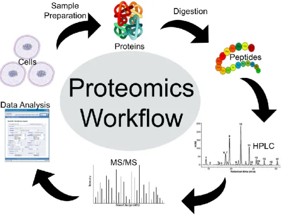
Before exploring proteomics techniques, is important to understand the pathway required to do from sample to protein identification. Figure 1.7 shows the workflow for a MS-based proteomics.
6
Figure 1.7: MS-based Proteomics workflow.(adapted)15
Being Proteomics currently such an enormous field, there is an array of techniques that can be used where some can depend on the final objective of the study.
Figure 1.8 illustrates a group of techniques used currently in Proteomics.
MS analysis is an important technique in Proteomics, and it has become the method of choice for complex protein sample analysis. This discipline was made possible by the existence of genome sequence databases and technical advances in many areas.16
7
Figure 1.8: Techniques in Proteomics.(adapted)14
1.5 Gel-based Proteomics:
There are three gel-based techniques in Proteomics. These techniques involve the use of intact proteins during all stages of analyses. As suggested by the name this technique is performed on a gel made of polyacrylamide. These three techniques are very similar, but they have an increased power of separation. 1-dimensional electrophoresis (1D-GE), 2-dimensional electrophoresis (2D-GE) and 2 dimensional electrophoresis difference gel (2D-DIGE) are the gel-based techniques (Table 1.1).14,17
1D-GE separates proteins in groups by molecular weight, 2D-GE separates proteins not only by molecular weight but also by isoelectric point.17,18,19
2D-DIGE has a different form of gel that is capable of separating up to three protein samples, reducing intergel variability. Fluorophores are needed for visualization of proteins.14,17
8
Table 1.1: Gel-based techniques strengths and limitations.14
Technology
Application
Strengths
Limitations
2D-GE
Protein separation
Quantitative expression
profiling
Relative quantitative
PTM information
Poor
separation
of acidic,
basis,
hydrophobic
and low
abundant
proteins
2D-DIGE
Protein separation
Quantitative expression
profiling
Relative quantitative
PTM information
High sensitivity
Reduction of
variability
Proteins
without
lysine
cannot be
labelled.
Expensive
1.6 Shotgun Proteomics:
Shotgun proteomics approaches use multi-dimensional capillary liquid chromatography combined with tandem mass spectrometry (MS/MS) to separate and identify the obtained peptides from the enzymatic digestion. It is important to notice that in shotgun proteomics it is not the protein that is separated. Instead of that protein are transformed into peptides by enzymatic digestion, and those peptides are separated and expose to MS/MS analysis. Once peptides are easier to separate by LC than proteins, shotgun proteomics are faster and cheaper than gel-based analysis.20
Shotgun proteomics has also isotopic labelling methods such as O18.14
1.7 Immobilized Trypsin:
Digestion is by far the most crucial step in protein identification and quantification.21
This concept refers to the enzymatic transformation of proteins into peptides. Although many enzymes can be used to perform protein digestion, trypsin is, by far, widely used.22
Trypsin cleaves peptide bonds at the carboxyl side of arginine and lysine. Therefore, this enzyme can produce a reproducible pool of peptides with an average size range between 600-2500 Da.23 Tryptic digestion can be performed in a heterogeneous or homogeneous phase. In the homogeneous phase, trypsin is in solution with the proteins. By contrast, the heterogeneous phase has the protein in solution, and the trypsin is immobilized onto a solid support. Immobilized trypsin prevents auto digestion of the enzyme avoiding downstream conflicts with MS analysis
9
and posterior protein identification. This technique also increases effective trypsin concentration which may result in shorter digestion times.21,24
Trypsin immobilization can occur in varied materials such as polymeric or metallic materials. Currently and independent of the material, these reactors are micro-sized.25
In this work, will be used a new and revolutionary type of immobilized trypsin. We will use iron nanoparticles with 80nm and magnetic properties where trypsin will be covalently attached to the nanoparticle. TEM image of the immobilized trypsin magnetic nanoparticles in Figure 1.9.
Figure 1.9: TEM picture of Immobilized Trypsin magnetic nanoparticles
1.8 Preconcentration of Phosphopeptides:
MS is currently the method of choice to detect changes in protein phosphorylation and to identify the position of specific phosphorylation events. However, even with the most recent advances in MS instrumentation, the detection and identification of phosphoproteins are compromised by a low ratio of phosphorylated and non-phosphorylated proteins. Only 1 to 2% of the entire protein amount is phosphorylated. Another issue is the phosphorylation cycles that may occur on a very short timescale.12,26
To be successful in such an endeavour, there is a prerequisite for an effective enrichment of phosphopeptides. New alternatives have been developed to overcome these issues.13 Figure 1.10 shows the most common techniques employed in the enrichment of phosphopeptides.
10
Figure 1.10: Common enrichment of phosphopeptides techniques.(adapted)27
Some alternative approaches have been performed to determine the phosphorylation stoichiometry. Conventionally, this has involved assessing the amount of 32P incorporation. However, this method is becoming less used nowadays due to safety constraints. Alternatively, protein phosphorylation can also be measured by MS. Typically, an enrichment step to pre-concentrate the low abundance phosphopeptides using immunoprecipitation, affinity purification, and strong cation exchange chromatography is required before MS analysis. However, these techniques are expensive, time-consuming, and a skilled operator is demanded to operate them. Immunoprecipitation techniques perform a decent enrichment however it has been proven to be highly applicable to samples containing peptides with phosphotyrosine.28
Immobilized metal affinity chromatography (IMAC) and metal oxide affinity chromatography (MOAC), were the first successful strategies developed for phosphopeptide enrichment. Both involve an immobilized metal ion or metal oxide, which is capable of coordination and has a high preference for phosphate groups. IMAC with Fe3+, Ga3+, or Ti4+, and MOAC mostly with TiO2 are nowadays the most-used enrichment methods for phosphopeptides.
Chemical coupling is a different approach for enrichment, in this technique phosphopeptides are covalently attached to a polymeric support. This requires multiple reactions steps and purification increasing the complexity of the technique and resulting in sample loss.10,13
Strong cation exchange (SCX) chromatography and IMAC are the most popular strategies. SCX is performed at very low pH (≈2.7) while phosphopeptides can remain negatively charged at this conditions allowing a major separation between phosphopeptides and nonphosphopeptides.13 Other authors consider this technique as a prefractionation technique rather than a enrichment
11
technique.27,29 While other authors refer that a combination of SCX followed by IMAC is the most successful technique.10
IMAC is considered to be the first truly successful technique for enrichment of phosphopeptides. This strategy involves an immobilized metal ion capable of coordinating specifically with phosphate groups due to its high preference for these groups. Iron and gallium metal ions are widely used. However, one of IMAC’s limitations is the nonspecific adsorption resulting of nonphosphopeptides containing multiple acidic amino acids such as glutamate and aspartate.13
1.9 Mass Spectrometry:
MS uses mass analysis for protein identification, and it is the most popular and versatile technique for large-scale proteomics. MS measures the mass to charge ratio (m/z) of gas-phase ions. Thus a mass spectrometer equipment consists of an ion source, converting molecules into gas-phase ions, a mass analyser, separating ions based on m/z, and a detector recording the number of ions of each m/z.30,31 Simple diagram in Figure 1.11.
Figure 1.11: Simple diagram of a mass spectrometer.(adapted)32
In a mass spectrometer, a form of energy ionizes and fragments a molecule; next, this molecule is accelerated by an electromagnetic field separating the fragments according to their m/z after that a detector counts the number of fragments of each m/z. Using a proper software, a graphic of abundance vs m/z is presented.32
12
1.10 Soft Ionization Techniques:
Matrix-assisted laser desorption/ionization (MALDI) and Electrospray ionization (ESI) are the two preferred techniques to ionize molecules for prior mass spectrometric analysis. Before soft ionization techniques become available, MS was not considered to perform in biological sciences.33 Common MALDI analytes are peptides, proteins and nucleotides; sample introduction is in a solid matrix. MALDI sublimates the dried samples out of a crystalline matrix through a laser beam, Figure 1.12.16,30,34
Figure 1.12: MALDI ionization technique.(adapted)35
Currently, MALDI is crucial in proteomics due to its sensitivity and simplicity besides this MALDI-TOF-MS (time of flight – TOF) accomplishes fast analysis generating amounts of date in a brief period. As stated before MALDI samples must be in matrixes, Figure 1.13 shows common matrixes used in MALDI.36
13
Figure 1.13: Common MALDI matrixes36
ESI is driven by high voltage (between 2 and 6 kV) applied between the emitter and the inlet of the mass spectrometer. ESI processes involve creation of electrically charged spray, trailed by formation and desolvation of sample droplets.30,33 Samples are insert in a liquid form.16,31
Figure 1.14: ESI ionization technique.35
1.11 Mass spectrometer analysers:
Mass analysers are a critical technology for MS. MS-based proteomics analysers are required to have high resolution, sensitivity and mass accuracy. There are four analysers commonly used in proteomics, ion trap, time of flight (TOF), quadrupole (Q) and orbitrap. These analysers can perform alone or together in MS/MS to take advantages of each analyser strength. Usually, MALDI is coupled with TOF, more recently TOF TOF or even triple quadrupole. ESI is coupled with ion trap or triple quadrupoles.36
TOF-TOF instruments incorporate a collision cell between the two TOF section. In the first TOF ions with a specific m/z are selected, next this selected are fragmented in the collision cell, in the second TOF the fragments created are separated.16 Illustration in Figure 1.15.
14
Figure 1.15: TOF-TOF analyser16
Ions of a selected m/z in a quadrupole mass spectrometer have a stable trajectory due to time-varying electric fields between four rods present in the equipment. Similar to TOF-TOF, in triple quadrupoles, ions of a specific m/z are selected in the first quadrupole, fragmented is the second quadrupole and separated on the third.16 Illustration in Figure 1.16.
Figure 1.16: Triple quadrupole analyser16
The quadrupole TOF (Qq-TOF) analysers combine the front part of a triple quadrupole with the reflector TOF for measuring the m/z.16 Illustration in Figure 1.17.
15
2 Objectives:
The work presented in this dissertation aims the development of a new nano-micro materials for mass spectrometry-based proteomics applications covering the key steps of protein digestion for identification of proteins by tandem MS as well as phosphopeptide enrichment for phosphoproteomics analysis. The topics covered by this research work include:
Optimization of the conditions for robust and reproducible protein digestion using immobilized nano-trypsin.
Synthesis of polystyrene nanoparticles using a 23 experimental design.
Synthesis of a nano-micro immobilized lanthanide metal ion affinity material for phosphopeptide enrichment.
Optimizing the experimental conditions for unbiased and reproducible phosphopeptide enrichment using new nano-micro immobilized lanthanide metal affinity chromatography.
17
3 Methods:
3.1 Preparation of a simple protein stock for tryptic digestion:
Reagents: Ammonium Bicarbonate (AmBic) 1M, Acetonitrile (ACN) (Carlo Erba Reagents),
Milli-Q Water (MMilli-QH2O), Bovine Serum Albumin (BSA) (Sigma-Aldrich), Ditiotreitol (DTT) (Nzytech) and Iodoacetamide (IAA) (Sigma-Aldrich)
Equipment: Vortex and Incubator
Procedure: In an Eppendorf dissolve 5mg of BSA in 1mL of MQH2O. From this prepared stock transfer to another Eppendorf 100μg of Protein (20μL of solution) then add 2μL of DTT 110mM, agitate and incubate for 45 minutes at 37˚C. Add 2μL of IAA 400mM, agitate and incubate for 35 minutes at RT in the dark. To finish, add 476μL of AmBic 12.5mM 2% ACN and vortex. At this point, samples can be freeze for future use.
3.2 Preparation of E.Coli lysates stock for tryptic digestion:
Reagents: Urea, AmBic 1M, ACN, DTT, IAA and MQH2O
Equipment: Centricon, Vortex, Centrifuge
Procedure: Transfer the lysates samples to a centricon to remove the buffer by centrifuge for 15 minutes at 6000rpm. Add 300μL of urea 3M dissolved in AmBic 12.5mM/2% ACN (pH ≈ 8.5) in the centricon and centrifuge for 15 minutes at 6000rpm. Next, add 100μL of urea 3M dissolved in AmBic 12.5mM/2% ACN and centrifuge for 15 minutes at 6000rpm and repeat. Remove the supernatant. This supernatant can be freeze for future analysis. Perform the Bradford technique to quantify the amount of protein in the samples. Transfer the desired amount of protein and add DTT 110mM to have 10mM of DTT in solution, vortex and incubate for 45 minutes at 37˚C. Add IAA 400mM to have in the final solution 33.33mM of IAA, vortex and incubate for 35 minutes at RT in a dark place. Add AmBic 12.5mM/2% ACN to reach a final volume of 500μL. Before tryptic digestion, urea must be removed from the solution using a Zip-Tip technique. Samples can be freeze for future use.
3.3 Bradford assay:
Reagents: BSA, MQH2O and Bradford Reagent (Sigma-Aldrich).
Equipment: Vortex, ClarioStar (Spectrophotometer), 96-well plate
Procedure: Prepare a working solution containing 2μg/μL of BSA. Using a 96-well plate
prepare the calibration curve in duplicates by loading 5μL of the solution prepared according to Table 3.1 and 250μL of Bradford reagent. To each well used, add 5μL of a sample with
18
appropriate dilution and 250μL of the Bradford reagent and mix. Measure the absorbance at 595 nm. The protein-dye complex is stable up to 60 minutes, assure your measure are before the time limit. Plot the net absorbance vs the protein concentration of each standard. Calculate the protein concentration of unknown samples by comparing the absorbance values against the standard curve ( Table 3.1)37,38.
Table 3.1: Calibration curve
Concentration (μg/μL) Volume of BSA 2μg/μL (μL) Volume of H2O (μL)
0 0 200 0.2 20 180 0.4 40 160 0.6 60 140 0.8 80 120 1 100 100 1.2 120 80 1.4 140 60
3.4 Zip-Tip Technique:
Reagents: ACN, MQH2O, Trifluoracetic acid (TFA) (Sigma-Aldrich), Formic Acid (FA) (Fluka Analytical) and Zip Tips (Thermo Scientific).
Equipment: Vortex
Procedure: First, aspirate 100μL of ACN and discard, repeat once. Aspirate 100μL of 0.1%
TFA and discard, repeat. Aspirate 100μL of the sample and do up and down ten times and discard. Aspirate 100μL of 0.1% TFA/2% ACN and discard, repeat. Elute the proteins with 5μL of 0.1% FA/50% ACN. Elute again now using 5μL of 0.1% FA/90% ACN.39
3.5 Tryptic digestion of simple protein using immobilized trypsin
nanoparticles:
Reagents: AmBic 1M, ACN, MQH2O, BSA and Immobilized Trypsin nanoparticles.
Equipment: Vortex, Ultra Sonic Bath (US) and Incubator
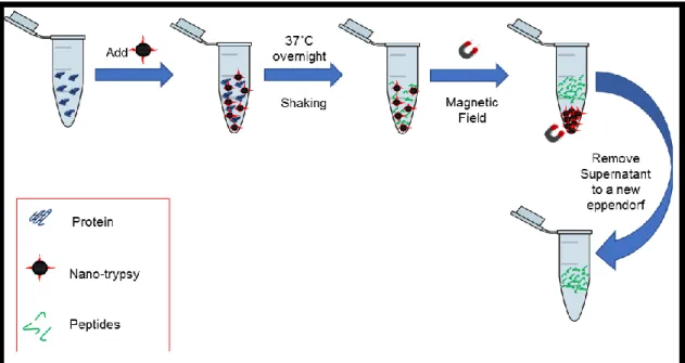
Procedure: Sonicate the stock of immobilized trypsin for 10 minutes. Prepare the target immobilized trypsin concentration. In an Eppendorf mix 1, 5 and 10μg (5, 25 and 50μL) of BSA with 20μL of immobilized trypsin and complete the volume using AmBic 12.5mM/2% ACN for a final volume of 120μL. Incubate the samples overnight with gentle stirring at 37˚C. Remove the samples from the incubator, shake and spin down them. With the help of a magnet separate the
19
supernatant from the pellet transferring the supernatant to a new Eppendorf. Samples can be freeze for future analysis. Figure 3.1 shows a quick walk-through for this technique.
Figure 3.1: Quick walk-through for tryptic digestion using immobilized trypsin magnetic nanoparticles.
3.6 Tryptic digestion of simple protein using commercial
immobilized trypsin microparticles:
Reagents: AmBic 1M, ACN, MQH2O, BSA and Commercial Immobilized Trypsin (ClonTech Laboratories).
Equipment: Vortex, Ultrasonic Bath (US) and Incubator
Procedure: Sonicate the immobilized trypsin for 10 minutes. Remove the amount of trypsin desired and wash with MQH2O twice. Prepare the target immobilized trypsin concentration. In an Eppendorf mix 1, 5 and 10μg (5, 25 and 50μL) of BSA with 20μL of immobilized trypsin and complete the volume using AmBic 12.5mM/2% ACN for a final volume of 120μL. Incubate the samples overnight with gentle stirring at 37˚C. Remove the samples from the incubator, shake and spin down them. With the help of a magnet separate the supernatant from the pellet transferring the supernatant to a new Eppendorf. Samples can be freeze for future analysis.
3.7 MALDI analysis of simple protein digestion for protein
identification:
Reagents: Ammonium dihydrogen phosphate (ADP) (Sigma-Aldrich) α-cyano-4-hydroxycinnamic acid (CHCA) (Fluka), ACN, MQH2O, TFA, FA.
20
Procedure: Dry the peptidic samples in the speed vacuum. Resuspend the samples in 10 μL
of 0.3% FA, vortex the samples, incubate for 15 minutes at 37˚C and vortex again. Prepare a stock solution by dissolving 10mg od ADP in 1 mL of MQH2O Prepare the MALDI matrix by dissolving 7mg of CHCA in a mixture of 100μL of Stock solution, 500μ of ACN, 400μL of MQH2O and 1μL of 0.1% TFA. In the MALDI target, placate 0.5μL of the sample and on the sample, placate 1μL of MALDI matrix. Samples in the MALDI target can be read after dried. What remains of samples can be freeze for future analysis.
3.8 ESI LC analysis proteins:
Reagents: FA, ACN, Equipment: Easy-nLC II
Procedure: Before ESI MS/MS analysis all samples were diluted with 100 μL of 0.1% (v/v) aqueous FA before loading onto an EASY-nLC II equipped with an EASY-Column, 2cm, ID100µm, 5µm, C18-A1 (Thermo Fisher Scientific) and an EASY-Column, 10cm, ID75µm, 3µm, C18-A2 (Thermo Fisher Scientific). Chromatographic separation was carried out using a multistep linear gradient at 300 nL/min (mobile phase A: aqueous formic acid 0.1% (v/v); mobile phase B 90% (v/v) ACN and 0.1% (v/v) FA) 0-90 min linear gradient from 0% to 35% of mobile phase B, 90-100 min linear gradient from 35% to 95% of mobile phase B. For each sample two replicate injections were performed.
MS acquisition was set to cycles of MS (2 Hz), followed by MS/MS (8–32Hz), cycle time 3.0 seconds, active exclusion, exclude after one spectrum, release after 0.5 min. Reconsider precursor if current intensity, previous intensity 3.0 an intensity threshold for fragmentation of 2000 counts. All spectra were acquired in the range 150–2200 Da. LC-MS/MS data were analysed using Data Analysis 4.2 software (Bruker).
Proteins were identified using Mascot (Matrix Science, UK). MS/MS spectra were searched against the SwissProt database 57.15 (515,203 sequences; 181,334,896 residues), setting the taxonomy to E.coli (22,646 sequences). Tandem MS data were searched with MASCOT search engine with the following parameters: precursor mass tolerance of 20 ppm, fragment tolerance of 0.05 Da, trypsin specificity with a maximum of 2 missed cleavages, cysteine carbamidomethylation set as fixed modification and methionine oxidation, as variable modification. Significance threshold for the identification was set to p < 0.05 and false discovery rate (FDR) was estimated by running the searches against a randomized decoy database. Results of the identification step were filtered to proteins with a FDR below 1%.40
Proteins were identified using Mascot (Matrix Science, UK). MS/MS spectra were searched against the SwissProt database 57.15 (515,203 sequences; 181,334,896 residues), setting the taxonomy to Other Mammalia (12,633 sequences). Tandem MS data were searched with MASCOT search engine with the following parameters: precursor mass tolerance of 20 ppm,
21
fragment tolerance of 0.05 Da, trypsin specificity with a maximum of 1 missed cleavage, cysteine carbamidomethylation set as fixed modification and methionine oxidation, serine, threonine and tyrosine phosphorylation as variable modification. Significance threshold for the identification was set to p < 0.05 and false discovery rate (FDR) was estimated by running the searches against a randomized decoy database. Results of the identification step were filtered to proteins with a FDR below 1%.40
3.9 Polyacrylamide gel
Reagents: Solution I, Solution II, Solution III, SDS 10%, Butanol 50% (Sigma-Aldrich), MQH2O, APS and TMED.
Equipment: Gel supporter Procedure:
Table 3.2: Polyacrylamide Gel Protocol.41
Stock Solution Stacking Gel Running Gel
% acrylamide 4 12
Solution I* - 2.5
mL
Solution II* 1 -
Solution III (acrylamide/bisacrylamide)
(37.5:1) 0.52 4 SDS 10% 0.04 0.1 H2O Milli-Q 2.48 3.4 APS 10 % 30 70 μL TMED 2 5
*Solution I: Tris-Base 27.23g, add HCl until pH=8.8 and MQH2O until 150mL; Solution II: Tris-Base 6.06g,
add HCl until pH=6.8 and MQH2O until 100mL
To produce the stacking gel and running gel mix the above quantities in a centrifugal tube. First, produce the running gel, place it in the gel supporter, add a 50% butanol solution to create a plane surface avoiding air entrance and wait for polymerization to occur. Next prepare the stacking gel and place it over the polymerized running gel, add the well comb and wait for polymerization. Keep in mind that polymerization time is about 15 to 30 minutes and it starts after mixing APS and TMED together. Remove the comb, and the gel is prepared.41
3.10 1D Gel Electrophoresis:
Reagents: 12.5% polyacrylamide gel Equipment: Gel supporters and electrodes.
Procedure: After sample clean up, protein samples were re-suspended in 10μL of 1x
Laemmli sample buffer and then heated in a dry bath at 100ºC for 5 minutes. The denatured proteins were loaded on 12.5% polyacrylamide gels with 1mm thickness. Proteins were
22
separated at 200 V(constant voltage) until the tracking dye front reaches the bottom of the gel.42,43
3.11 Gel staining and image analysis
Reagents: Ethanol (Carlo Erba Reagents), acetic acid (Panreac), Coomassie blue G-250m
distilled H2O and NaCl 0.5M
Equipment: No specific equipment
Procedure: Finished the gel electrophoresis, the gel was fixed for 30 minutes with 40% (v/v) ethanol and 7.5% (v/v) acetic acid and then stained overnight with colloidal Coomassie blueG-250. Gels were rinsed 4×20 min with 100mL of distilled water and further washed twice with 100 mL of 0.5 M sodium chloride until a clear background was observed. Gel imaging was carried out with a ProPicII–robot using 16ms of exposure time and a resolution of 70μm.44
3.12 Synthesis of polystyrene nanoparticles:
Reagents: Ammonium Persulfate (APS) (Sigma-Aldrich), Sodium Dodecyl Sulphate (SDS)
(Panreac), MQH2O, Styrene and 1-penthanol.
Equipment: Heating mantle, thermometer, mini pump, vortex, US bath, Round-bottom flasks,
centrifuge tubes and speed vacuum.
Procedure: Dissolve APS and SDS in MQH2O. Sonicate the mixture to assure a good and fast dissolution. Transfer the solution to a round-bottom flask and increase the temperature to 80˚C while stirring at 1000rpm. After reach 80˚C start adding, at constant rate, a mix of styrene and 1-penthanol for 30 minutes. After all styrene been added, maintain the temperature between 80 and 85˚C for 1 hour. Filtrate the obtained solution through a 220nm pore filter to a centrifugal tube. To quantify the amount of seeds, present in solution, assure a good homogenization and remove and dry 1mL of the solution, weight the precipitate keeping in mind that the precipitate has Seeds and SDS. As soon as possible clean the flask with xylene, dried styrene can be a hard to remove.
Quantities of APS, SDS, MQH2O and Styrene vary according to the experience performed, Table 3.3 provides quantity of reagents for each experience.45
23
Table 3.3: Amount of reagents for each experience.
Experiment APS (g) SDS (g) Styrene (mL) 1-Penthanol
(mL) MQH2O (mL) 1 0.004 0.2 0.7 0.01 48.3 2 0.04 0.2 0.7 0.01 48.3 3 0.004 2 0.7 0.01 48.3 4 0.04 2 0.7 0.01 48.3 5 0.004 0.2 7 0.1 42 6 0.04 0.2 7 0.1 42 7 0.004 2 7 0.1 42 8 0.04 2 7 0.1 42
3.13 Synthesis of monodisperse nano spheres-based immobilized
lanthanides ion affinity chromatography:
Reagents: Polystyrene nano spherical seeds (Seeds), Polyvinyl Alcohol (PVA) (Sigma-Aldrich),
Glycidyl Methacrylate (GMA) (Sigma-Aldrich), Trimethylolpropane Trimethacrylate (TMPTMA) (Sigma-Aldrich), 2,2'-Azobis(2-methyl-propionitrile) (AIBN) (Sigma-Aldrich), Toluene (Panreac), Tetrahydrofuran (THF) (Carlo Erba Reagents), Acetone (Sigma-Aldrich), Ethylenediamine (Scharlau), Ethanol, MQH2O, ACN, TFA, Phosphoric acid (Alfa Aesar), HCl (), Formaldehyde (Panreac) Titanium Chloride Aldrich) and Lanthanum Chloride Heptahydrate (Sigma-Aldrich).
Equipment: Round-bottom flasks, heating mantle, condensation column, thermometer,
centrifugal tubes, rotavapor and centrifuge.
Procedure: Prepare a 15mL solution containing 450mg of seeds and 1% (w/w) PVA and 0.25% (w/w) SDS, sonicate the solution to homogenise. Prepare a 150mL solution containing 1% (w/w) PVA and 0.25% (w/w) SDS. Prepare an oil-phase solution adding 6.7mL of GMA, 6.7mL of TMPTMA, 140mg of AIBN and 16.6mL of toluene. Add the oil-phase solution with 150mL of the seedless solution and sonicate for 10 minutes or more assuring that an emulsion is created. Add this new solution to the seeds in a round-bottom flask. Start stirring at 1200rpm. Increase the temperature to 30 ˚C. Maintain this condition for 20 hours to perform seed swelling. Increase the temperature now to 70˚C to start the polymerization, keep the stirring. Reaction time is 24 hours. Transfer the obtained solution to centrifugal tubes and wash with 15mL of THF and 15mL of acetone for each tube. Repeat the washes five times. Dry the solution in the rotavapor. Add 7g of this new dried compound with 150mL of ethylenediamine in a round-bottom flask. The reaction is conducted at 80˚C, 1200 rpm for 3 hours. Transfer the obtained solution to centrifugal tubes and wash with 30mL of 50% Ethanol, repeat the washes five times. Dry the solution in the rotavapor.
24
Add 7g of the last compound obtained with 5.1mL of phosphoric acid, 10mL of 37%HCl and 8mL of formaldehyde successively. Increase the temperature to 100 ˚C and stir at 1200rpm. Maintain these conditions for 24 hours. Transfer the solution to centrifugal tubes and wash each one with 30mL of 50% Ethanol, wash five times. Dry the solution in the rotavapor. The compound produced can be stored at RT for several months avoiding the light. Incubate 100mg of this compound with 20mL of a solution of the chosen metal (0.09M in 20% HCl). Stir at 1200rpm for 8 hours at RT. Transfer the solution to centrifugal tubes and wash with 10mL of 30% ACN and 0.1% TFA, wash five times.13 Reaction scheme in Figure 3.2.
25
3.14 Enrichment of phosphopeptides using an IMAC column:
Reagents: Methanol (Carlo Erba Reagents), FA, Loading Buffer 1 (80% ACN/6%TFA) (pH ≈ 1),
Washing Buffer 1 (50% ACN/0.5% TFA/200mM NaCl) (pH ≈ 2), Washing Buffer 2 (50% ACN/0.1% TFA) (pH ≈ 2), Elution Buffer 1 (10% Ammonium) (pH ≈ 12) and Elution Buffer 2 (80%
ACN/2% FA) (pH ≈ 3).
Equipment: C8 (Supelco), vortex and centrifuge.
Procedure: Place a C8 membrane in a 10μL tip and wash with 20μL of methanol. Add multiples of 50μL of IMAC with a concentration of 10mg/mL until reach the target amount. For each time of IMAC added centrifuge at 200G for 2.5 minutes. Equilibrate the IMAC with 50μL of Loading Buffer, centrifuge at 200G for 2.5 minutes and repeat this step. Add 100μL of sample and centrifuge at 20G for 6 minutes. Wash the IMAC column with 50μL of Washing Buffer 1, centrifuge at 100G for 4 minutes. Wash the IMAC a second time using 50μL of Washing Buffer 2, centrifuge at 100G for 4 minutes. In a new Eppendorf add 35μL of 10% FA and elute the phosphopeptides with 20μL of Elution Buffer 1, centrifuge at 100G for 3 minutes. Preform the second elution using 20μL of Elution Buffer 2, centrifuge at 100G for 3 minutes. Add 3μL of FA to acidify the sample, perform a Zip-Tip to remove salts and impurities from the sample. Samples can be freeze for further use.13
27
4 Results and Discussion:
4.1 Protein digestion with immobilized trypsin:
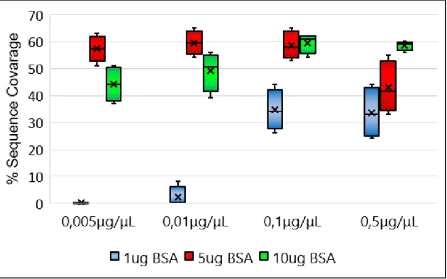
To perform protein digestion, trypsin, was the chosen enzyme. As already stated trypsin is the desired enzyme due to its specificity. Trypsin was immobilized in a nanoparticle (80nm) with an iron core that confers magnetic properties to this particle. Since this immobilized trypsin device is brand new and has never been tested, it is imperative to evaluate its performance. In the first phase, it was important to discover how the device responded in general conditions since the amount of trypsin per mg of nanoparticle was unknown. Therefore, a large array of protein and immobilized trypsin concentrations were tested. BSA was used as a reference because it is a simple protein with a molecular weight of 66 kDa46, which is easy to digest. Digestion success will be evaluated by sequence coverage percentage, a higher sequence coverage implies a good digestion. To assess the efficiency of this immobilized trypsin, BSA was digested in the following conditions: 4 different concentrations of trypsin (0.005, 0.01, 0.1 and 0.5 mg/mL) and three different amounts of protein (1, 5 and ten μg). The ratios of particles of immobilized enzyme to protein are between 1:0.02 and 1:17. The ratio of enzyme-protein for in-solution digestion with trypsin is usually 1:20. According to the provided procedure, commercial immobilized trypsin microparticles should be used at a concentration of 5% (w/w). Results in Figure 4.1 and important MS spectra in Figures 4.2 and 4.3.
Figure 4.1: Sequence Coverage of the digestion of 1, 5 and 10 μg of BSA using 0.005, 0.01, 0.1 and 0.5μg/μL of Immobilized trypsin nanoparticles.
28
Protein identification was successfully achieved in these range of protein and enzyme concentrations, except when the lowest concentrations of protein and enzyme are combined (1μg of protein and 0.005μg/μL of nanoparticle), extreme conditions are rarely used, therefore, this will not be considered as a failure, but as the limitation of the system. Also, sequence coverage above 60% proves that digestion performance is quite good. Results also highlight the concentration of nanoparticles which assure better digestion and, therefore, a higher percentage of sequence coverages and possibly better identifications, ratios of immobilized trypsin particles to protein of 1:4 or 1:1 have higher percentages of sequence coverage. When 0.005μg/μL and 1μg of BSA were used, no identification was made, with 0.01μg/μL and 1μg of BSA only one identification was made. In all the remain conditions four identifications were possible to make; four replicates were make.
Other mass spectra of this experiment can be found in Annex I
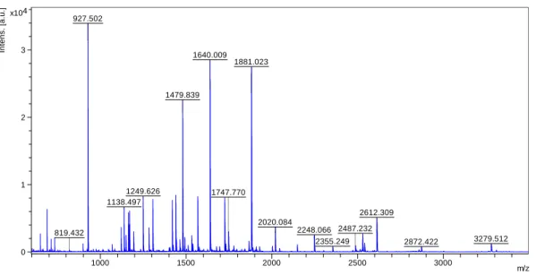
Figure 4.2: MS spectrum of the digestion of 1μg of BSA with 0.005μg/μL of immobilized trypsin nanoparticles.
Figure 4.3: MS spectrum of the digestion of 5μg of BSA with 0.1μg/μL of immobilized trypsin nanoparticles. 1193.636 927.529 1443.659 0 500 1000 1500 2000 2500 3000 In te n s . [a .u .] 1000 1500 2000 2500 3000 m/z 927.502 1640.009 1881.023 1479.839 1249.626 1138.497 2612.309 2020.084 1747.770 2248.066 2487.232 3279.512 2355.249 2872.422 819.432 0 1 2 3 4 x10 In te n s . [a .u .] 1000 1500 2000 2500 3000 m/z
29
Although this system works, it was still needed to assure its reproducibility.
In the following experimentation, four batches of immobilized trypsin were prepared. To test the reproducibility of the device, two different concentrations of immobilized trypsin nanoparticles and two separate amounts of protein were used and, therefore, four different enzyme-protein ratios were tested. For each condition, four replicates were made. Results in Figures 4.4, 4.9, 4.10 and 4.11 and significant MS spectra in Figures 4.5, 4.6, 4.7 and 4.8.
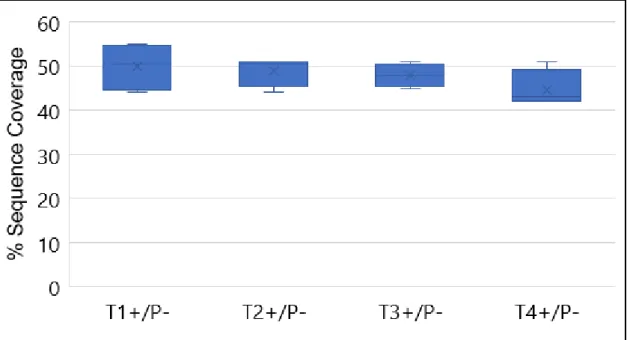
Figure 4.4: % Sequence Coverage of the digestion of 10μg of BSA with 0.5μg/μL of 4 different batches of immobilized trypsin nanoparticles.
Figure 4.5: MS spectrum of the digestion of 10μg of BSA with 0.5μg/μL of immobilized trypsin nanoparticles – batch 1. 927.481 1639.942 1479.791 1283.691 1880.937 1170.602 2045.038 2612.269 1747.720 2247.959 3000.570 0.0 0.5 1.0 1.5 4 x10 In te n s . [a .u .] 1000 1500 2000 2500 3000 m/z
30
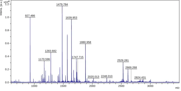
Figure 4.6: MS spectrum of the digestion of 10μg of BSA with 0.5μg/μL of immobilized trypsin nanoparticles – batch 2.
Figure 4.7: MS spectrum of the digestion of 10μg of BSA with 0.5μg/μL of immobilized trypsin nanoparticles – batch 3. 1479.784 927.486 1639.953 1880.958 1283.682 1170.596 2529.281 2248.010 1747.715 2020.013 2824.431 2669.268 0.0 0.2 0.4 0.6 0.8 1.0 1.2 4 x10 In te n s . [a .u .] 1000 1500 2000 2500 3000 m/z 1639.932 1439.786 927.494 1283.684 1880.905 1178.531 2529.233 2045.012 3000.508 0 2000 4000 6000 8000 In te n s . [a .u .] 1000 1500 2000 2500 3000 m/z
31
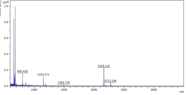
Figure 4.8: MS spectrum of the digestion of 10μg of BSA with 0.5μg/μL of immobilized trypsin nanoparticles – batch 4.
Figure 4.9: % Sequence Coverage of the digestion of 10μg of BSA with 0.1μg/μL of 4 different batches of immobilized trypsin nanoparticles.
2163.110 805.428 1153.572 2273.138 1493.729 0.0 0.2 0.4 0.6 0.8 1.0 4 x10 In te n s . [a .u .] 1000 1500 2000 2500 3000 m/z
32
Figure 4.10: % Sequence Coverage of the digestion of 1μg of BSA with 0.5μg/μL of 4 different batches of immobilized trypsin nanoparticles.
Figure 4.11: % Sequence Coverage of the digestion of 1μg of BSA with 0.1μg/μL of 4 different batches of immobilized trypsin nanoparticles.
Other mass spectra of this experiment can be found in Annex II
To ensure similarity between all the different batches, t-tests were performed for all batches and all enzyme-protein ratios. To decide whether the difference between two means, X1 and X2, is significant, to test the null hypothesis where H0: u1=u2 the statistic t is then calculated from Equation 1 (Annex III).
If the standard deviations, s1 and s2 are not significantly different, this assumption must be tested, s can be calculated using Equation 2 (Annex III).
33
To check if s1 and s2 are not significantly different, F test must be tested using Equation 3 (Annex III).
If F exceeds a critical value, s1 and s2 are significantly different, and therefore equation 1 cannot be used instead Equation 4 (Annex III) must be employed.
In Annex III results are displayed. All the batches are equal between them at a level of significance of 5%.47
Now it is possible to validate the efficiency and reproducibility of these immobilized trypsin nanoparticles.
Taking into consideration that the ratio of enzyme-protein has already been optimized, this ratio will be used for all the subsequent experiments.
However, in an attempt to increase sequence coverage and digestion speed, other variables were tested. In the following experience, stirring while samples are incubated overnight was analysed. Stirring improves the reaction giving motion to the immobilized trypsin nanoparticles. Otherwise, they would deposit, which would reduce the surface of contact and therefore the digestion efficiency as well. Results in Figures 4.12 and 4.13 and important MS spectra in Figures 4.14 and 4.15.
Figure 4.12: % Sequence Coverage of the digestion of 10 μg of BSA and 0.6, 12 and 60 μg of immobilized trypsin nanoparticles while stirring and non-stirring.
0
10
20
30
40
60
12
0,6
38
35
28
38
37
32
%
Seqeunce
C
ov
erage
μg of particles
No Stirring
Stirring
34
Figure 4.13: % Sequence Coverage of the digestion of 1 μg of BSA and 0.6, 12 and 60 μg of immobilized trypsin nanoparticles while stirring and non-stirring.
Figure 4.14: MS spectrum of the digestion of 1μg of BSA with 0.6μg of immobilized trypsin nanoparticles, non-stirring while digestion.
0
10
20
30
40
50
60
60
12
0,6
48
43
28
50
52
43
%
Seqeunce
C
ov
erage
μg of particles
No Stirring
Stirring
1640.017 1193.597 927.389 1880.974 1479.844 811.431 2612.227 3000.507 0.0 0.5 1.0 1.5 2.0 2.5 4 x10 In te n s . [a .u .] 1000 1500 2000 2500 3000 m/z35
Figure 4.15: MS spectrum of the digestion of 1μg of BSA with 0.6μg of immobilized trypsin nanoparticles, stirring while digestion.
Other mass spectra of this experiment can be found in Annex IV
Sequence coverage increased when stirred, particularly when concentration of proteins and enzyme are very low. Therefore, stirring is now included in the process.
Many of immobilized trypsin systems try to not only avoid trypsin proteolysis, but also decrease the time of digestion.24,25 Overnight digestion (around 12 hours) delay results for one day. The next set of experiments examined how sequence coverage responded to a decrease in digestion time. Commercial immobilized trypsin particles efficiency has begun to be compared to our immobilized trypsin nanoparticles. Results in Figures 4.16 and significant MS spectra in Figures 4.17 and 4.18.
Figure 4.16: % Sequence Coverage of the digestion of 10μg of BSA and 0.5μg/μL immobilized trypsin nanoparticles, digestion time of 30 minutes, 1 hour, 2 hours and 6 hours.
1639.969 927.478 1195.590 1479.812 1880.938 811.598 1083.578 2045.042 1305.693 1747.694 2355.164 2612.212 3000.488 0 1 2 3 4 x10 In te n s . [a .u .] 1000 1500 2000 2500 3000 m/z