Parallel Implementation of a Two-level Algebraic ILU(k)-based Domain

doi: 10.5540/tema.2018.019.01.0059

Parallel Implementation of a Two-level Algebraic ILU(k)-based Domain

Decomposition Preconditioner

I.C.L. NIEVINSKI1*, M. SOUZA2, P. GOLDFELD3, D.A. AUGUSTO4, J.R.P. RODRIGUES5and L.M. CARVALHO6

Received on November 28, 2016 / Accepted on September 26, 2017

ABSTRACT. We discuss the parallel implementation of a two-level algebraic ILU(k)-based domain de-composition preconditioner using the PETSc library. We present strategies to improve performance and minimize communication among processes during setup and application phases. We compare our imple-mentation with an off-the-shelf preconditioner in PETSc for solving linear systems arising in reservoir simulation problems, and show that for some cases our implementation performs better.

Keywords: Two-level preconditioner, domain decomposition, Krylov methods, linear systems, parallelism, PETSc.

1 INTRODUCTION

This paper discusses the formulation and the parallel implementation of an algebraic ILU(k)-based two-level domain decomposition preconditioner first introduced in [2].

In this work we present and discuss details of the implementation using the MPI-based PETSc suite [3], a set of data structures and routines for the parallel solution of scientific applications modeled by partial differential equations. We also present results of computational experiments involving matrices from oil reservoir simulation. We have tested with different number of pro-cesses and compared the results with the default PETSc preconditioner, block Jacobi, which is a usual option in the oil industry.

†_{This article is based on work presented at CNMAC2016.}

*Corresponding author: ´Italo Nievinski – E-mail: italonievinski@gmail.com.

1Faculdade de Engenharia Mecˆanica, PPGEM, UERJ - Universidade do Estado do Rio de Janeiro, 20550-900 Rio de Janeiro, RJ, Brasil.

2Departamento de Estat´ıstica e Matem´atica Aplicada DEMA UFC - Universidade Federal do Cear´a, Campus do PICI, 60455-760, Fortaleza, CE, Brasil. E-mail: michael@ufc.br

3Departamento de Matem´atica Aplicada, IM-UFRJ, Caixa Postal 68530, CEP 21941-909, Rio de Janeiro, RJ, Brasil. E-mail: goldfeld@ufrj.br

4Fundac¸˜ao Oswaldo Cruz, Fiocruz, Av. Brasil, 4365, 21040-360 Rio de Janeiro, RJ, Brasil. E-mail: daa@fiocruz.br 5PETROBRAS/CENPES Av. Hor´acio Macedo 950, Cidade Universit´aria, 21941-915 Rio de Janeiro, RJ, Brasil. E-mail: jrprodrigues@petrobras.com.br

The multilevel preconditioner has been an active research area for the last 30 years. One of the main representatives of this class is the algebraic multigrid (AMG) method [19, 22, 30, 31], when used as a preconditioner rather than as a solver. It is widely used in oil reservoir simulation as part of the CPR (constrained pressure residual) preconditioner [6, 33]. Despite its general acceptance there is room for new alternatives, as there are problems where AMG can perform poorly, see, for instance [13]. Among these alternatives we find the two-level preconditioners. There are many variations within this family of preconditioners, but basically we can discern at least two subfamilies:algebraic[1, 4, 12, 14, 18, 20, 23, 28, 32] andoperator dependent[15, 16, 17]. Within the operator dependent preconditioners we should highlight the spectral methods [21, 25].

Incomplete LU factorization ILU(k) [26] has long been used as a preconditioner in reservoir simulation (an ingenious parallel implementation is discussed in [11]). Due to the difficulty in parallelizing ILU(k), it is quite natural to combine ILU(k) and block-Jacobi, so much so that this combination constitutes PETSc’s default parallel preconditioner [3]. The algorithm proposed in [2], whose parallel implementation we discuss in this article, seeks to combine the use of (sequential) ILU(K) with two ideas borrowed from domain decomposition methods: (i) the in-troduction of an interface that connects subdomains, allowing, as opposed to block-Jacobi, for the interaction between subdomains to be taken into account, and (ii) the introduction of a sec-ond level, associated to a coarse version of the problem, that speeds up the resolution of low frequency modes. These improvements come at the cost of greater communication, requiring a more involved parallel implementation.

The main contribution of the two-level preconditioner proposed in [2] is the fine preconditioner, as the coarse level component is a quite simple one. Accordingly, the main contribution in our article is the development of a careful parallel implementation of that fine part; nonetheless, we also take care of the coarse part by proposing low-cost PETSc-based parallel codes for its construction and application. Besides the parallel implementation, we present and discuss a set of performance tests of this preconditioner for solving synthetic and real-world oil reservoir simulation problems.

The paper is organized as follows. Section 2 introduces the notation used throughout the paper. Section 3 describes in detail the proposed two-level algebraic ILU(k)-based domain decompo-sition preconditioner, which we call iSchur. Its parallel implementation is detailed in Section 4, including the communication layout and strategies to minimize data transfer between processes, while results of performance experiments and comparisons with another preconditioner are pre-sented and discussed in Section 5. The conclusion is drawn in Section 6 along with some future work directions.

2 NOTATION

In this section, we introduce some notation that will be necessary to define iSchur.

Consider the linear system of algebraic equations

Ax=b (2.1)

arising from the discretization of a system of partial differential equations (PDEs) modeling the multiphase flow in porous media by a finite difference scheme withn gridcells. We denote by

ndofn×ndofn. For instance, for the standard black-oilformulation, see [24], the DOFs are oil

pressure, oil saturation and water saturation, so thatndof=3.

It will be convenient to think ofAas ablock-matrix:

A=

     

a11 a12 · · · a1n a21 a22 · · · a2n

..

. ... . .. ...

an1 an2 · · · ann

      ,

where ablock, denotedai j, is a matrix of dimensionndof×ndof.

The block-sparsity pattern ofAis determined by the stencil of the finite-difference scheme used for the discretization of the PDEs. Figure 1 depicts a bidimensional domain discretized by a 3×3 mesh and the sparsity pattern of the associated matrix for the black-oil model, assuming a five-point finite-difference stencil. We say that two gridcellsiand jare neighbors if either one of the blocksai jorajiis not null. For the five-point stencil, gridcells are neighbors when they share an

edge. The gridcells and their respective indices are identified, in a way thatΩdenotes either the

1 2

5 3

6 4

8 9

7

(a) 3×3 grid. (b) Associated matrix.

Figure 1: Discretization grid and associated matrix, assuming three unknowns per gridcell and a five-point stencil.

domain of the PDE or the set of indices{1,2, . . . ,n}. We introduce a disjoint partition ofΩ, i.e., we breakΩ={1,2, . . . ,n}intoPpiecesΩ₁,Ω2, . . . ,ΩP, in such a way that each gridcell belongs

to exactly one subdomainΩ_k, see Figure 2. More precisely, we define

{Ω_J}1≤J≤P s.t. P [

J=1

Ω_J=Ω and Ω_I∩Ω_J=/0 ∀I6=J. (2.2)

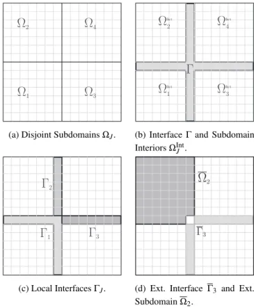
We note that there are gridcells that, while belonging to one subdomain, have neighbors in other subdomains. Our domain decomposition approach requires the definition of disconnected subdo-mains, that can be dealt with in parallel. For that sake, we define a separator set, called interface and denoted byΓ, and (disconnected) subdomain interiorsΩInt

J . A gridcell jis said to belong to

Γif it is in a subdomainΩ_Jwhile being neighbor of at least one gridcell in another subdomain with greater index, i.e.,Ω_K withK>J:

Ω

Ω

Ω

Ω

(a) Disjoint SubdomainsΩJ.

Ω

Ω

1

Ω

In t 3

Ω

Γ

(b) InterfaceΓ and Subdomain InteriorsΩInt

J .

Γ

Γ

Γ

(c) Local InterfacesΓJ.

Ω

Γ3

(d) Ext. Interface Γ3 and Ext. SubdomainΩ₂.

Figure 2: 2D Domain partitioned into 4 subdomains.

We now define the subdomain interiorΩInt

J as the portion ofΩJnot inΓ:

ΩInt

J =ΩJ−Γ, (2.4)

see Figure 2. These definitions are just enough to ensure that if gridcell jis inΩInt

J and gridcell kis inΩInt

K , withJ6=K, then they are not neighbors.1Indeed, to fix the notation, assumeJ<K.

Since j∈ΩInt

J ⊂ΩJandk∈ΩIntK ⊂ΩK, ifjandkwere neighbors, jwould be inΓby definition

(2.3) and therefore not inΩInt

J .

We now define the local interfaceΓ_Jassociated with each subdomainΩ_Jas the intersection ofΓ

andΩ_J, or equivalently,

ΓJ=j∈ΩJ

∃K>J and ∃k∈ΩK s.t. (ajk6=0 or ak j6=0) . (2.5)

Notice that{Γ_J}1≤J≤Pform a disjoint partition ofΓ. See Figure 2.

Finally, we define extended subdomainsΩ_Jand extended local interfacesΓ_J, which incorporate the portions of the interface connected to the subdomain interiorΩInt

J . We defineΩJas

Ω_J=Ω_J∪k∈Γ∃j∈ΩInt_J s.t. (ajk6=0 or ak j6=0) . (2.6)

1_{Had the conditionK>Jbeen dropped from definition (2.3),Γwould still be a separator set. But it would be unnecessarily}

andΓ_Jas its restriction toΓ, i.e.,Γ_J=Γ∩Ω_J, see Figure 2.

Notice thatΓ_J⊂Γ_J⊂Γ. We point out thatΓ_Jis the result of augmentingΓ_J with the gridcells of the interfaceΓthat are neighbors of gridcells inΩ_J. We refer toΓ_J as an extended interface, see Figure 2.

If the equations/variables are reordered, starting with the ones corresponding toΩInt

1 , followed

by the otherΩInt

J and finally byΓ, thenAhas the following block-structure:

A=

     

A11 A1Γ

. .. .._.

APP APΓ

AΓ1 · · · AΓP AΓΓ

     

, (2.7)

where the submatricesAJJ contain the rows and columns ofAassociated withΩInt_J ,AΓΓthe ones

associated with Γ,AJΓthe rows associated withΩInt_J and the columns associated withΓ, and

AΓJthe rows associated withΓand the columns associated withΩIntJ . Therefore, denoting by|S|

the number of elements in a setS, the dimensions ofAJJ,AΓΓ,AJΓandAΓJ are, respectively, ndofnJ×ndofnJ,ndofm×ndofm,ndofnJ×ndofm, andndofm×ndofnJ, wherenJ=

ΩInt

J

andm=

|Γ|. It is important to notice that, sincea_jk=0 for any j∈ΩInt

J andk∈ΩIntK withJ6=K, the

submatricesAJKof rows associated withΩIntJ and columns associated withΩIntK are all null (and

therefore omitted in (2.7)). This block-diagonal structure of the leading portion of the matrix (which encompasses most of the variables/equations) allows for efficient parallelization of many tasks, and was the ultimate motivation of all the definitions above. We point out that although not necessary by the method, the implementation discussed in this work assumes that the matrix A is structurally symmetric2, in this case the matricesAJJ andAΓΓare also structurally symmetric.

Furthermore,AJΓandAT_ΓJhave the same nonzero pattern.

3 DESCRIPTION OF THE TWO-LEVEL PRECONDITIONER

The goal of a preconditioner is to replace the linear system (2.1) by one of the equivalent ones:

(MA)x=Mb (left preconditioned) or

(AM)y=b (right preconditioned, wherex=My).

A good preconditioner shall renderAMorMAmuch better conditioned thanA(i.e.,Mshould approximate, in a sense, A−1_{) and, in order to be of practical interest, its construction and}

application must not be overly expensive.

We now present our preconditioner, which combines ideas from domain decomposition meth-ods, DDM, and level-based Incomplete LU factorization, ILU(k). In DDM, one tries to build an approximation to the action ofA−1based on the (approximation of) inverses of smaller, local ver-sions ofA(subdomain-interior submatricesAJJ, in our case). In this work, the action of the local

inverses is approximated by ILU(kInt), while other components required by the preconditioner

(see equation (3.4)) are approximated with different levels (kBord,kProd orkΓ). The motivation

for this approach is that ILU(k) has been widely used with success as a preconditioner in reser-voir simulation and DDM has been shown to be an efficient and scalable technique for parallel architectures.

It is well established that in linear systems associated with parabolic problems, the high-frequency components of the error are damped quickly, while the low-high-frequency ones take many iterations to fade, see [31]. In reservoir simulation, the pressure unknown is of parabolic nature. A two-level preconditioner tackles this problem by combining a “fine” preconditioner component

MF, as the one mentioned in the previous paragraph, with a coarse componentMC, the purpose

of which is to annihilate the projection of the error onto a coarse space (associated with the low frequencies). If the two components are combined multiplicatively (see [29]), the resulting two-level preconditioner is

M=MF+MC−MFAMC. (3.1)

In Subsection 3.1 we present a ILU(k)-based fine component MF and in Subsection 3.2 we

describe a simple coarse component.

3.1 ILU(k) based Domain Decomposition

The fine component of the domain decomposition preconditioner is based on the following block LU factorization ofA:

A=LU=

      L1 . .. LP B1 · · · BP I

           

U1 C1

. .. .._.

UP CP

S       , (3.2)

whereAJJ=LJUJis the LU factorization ofAJJ,BJ=AΓJUJ−1,CJ=L−J1AJΓand

S=AΓΓ−

P

∑

J=1

AΓJA−JJ1AJΓ=AΓΓ−

P

∑

J=1

BJCJ, (3.3)

is the Schur complement ofAwith respect to the interior points.

From the decomposition in (3.2), we can show that the inverse ofAis

A−1=      

U₁−1

. ..

U_P−1 I             C1

I ...

CP −I            I

S−1

          I

B1 · · · BP −I

          

L−₁1

. ..

L−_P1 I       . (3.4)

We want to define a preconditionerMF approximating the action ofA−1 on a vector.

S−1. These approximations are denoted byeL−_J1,Ue_J−1,BeJ,CeJ, andS−F1, respectively. The fine

preconditioner is then defined as

MF=

      e

U₁−1

. .. e

U_P−1

I             e C1

I ... e CP −I            I

S−_F1

          I e

B1 · · · BeP −I

           e

L−₁1

. .. e

L−_P1

I       . (3.5)

In the remaining of this subsection, we describe precisely how these approximations are chosen.

First we defineeLJ andUeJas the result of the incomplete LU factorization ofAJJ with level of

fill kInt,[eLJ,UeJ] =ILU(AJJ,kInt). In our numerical experiments, we usedkInt=1, which is a

usual choice in reservoir simulation. Even thougheLJ andUeJ are sparse, eLJ−1AJΓandUe_J−TATΓJ

(which would approximateCJ andBTJ) are not. To ensure sparsity,CeJ≈eL−J1AJΓ is defined as

the result of the incomplete triangular solve with multiple right-hand sides of the systemeLJCeJ= AJΓ, by extending the definition oflevel of fillas follows. Letvl andwl be the sparse vectors

corresponding to thel-th columns ofAJΓ andCerespectively, so that eLJwl =vl. Based on the

solution of triangular systems by forward substitution, the components ofvl andwl are related

by

wlk=vlk−

k−1

∑

i=1 e

LJkiwli. (3.6)

The level of fill-in of componentkofw_lis defined recursively as

Lev(wlk) =min

Lev(vlk), min 1≤i≤(k−1)

Lev(eLJki) +Lev(wli) +1

, (3.7)

where Lev(vlk) =0 whenvlk6=0 and Lev(vlk) =∞otherwise, and Lev(eLJki)is the level of fill of

entrykiin the ILU(kInt)decomposition ofAJJ wheneLJki6=0 and Lev(eLJki) =∞otherwise. The

approximationCeJ toCJ=L−J1AJΓis then obtained by an incomplete forward substitution (IFS)

with level of fillkBord, in which we do not compute any terms with level of fill greater thankBord

during the forward substitution process. We denoteCeJ=IFS(eLJ,AJΓ,kBord). Notice that when kBord=kInt,CeJ is what would result from a standard partial incomplete factorization ofA. The

approximationBeJtoBJ=AΓJUeJ−1is defined analogously.

Similarly, in order to define an approximationSetoS, we start by definingFJ=BeJCeJand a level

of fill for the entries ofFJ,

Lev(FJkl) =min

Lev(AΓΓ_kl), min

1≤i≤m

Lev(BeJki) +Lev(CeJil) +1

wherem=#ΩInt

J is the number of columns inBeJand rows inCeJ, Lev(AΓΓ_kl) =0 whenAΓΓ_kl6=0

and Lev(AΓΓkl) =∞, otherwise, and Lev(CeJki)is the level of fill according to definition (3.7)

whenCeJki6=0 and Lev(CJki) =∞, otherwise Lev(BeJil)is defined in the same way

. Next,FeJis

defined as the matrix obtained keeping only the entries inFJwith level less than or equal tokProd

according to (3.8). We refer to thisincomplete product(IP) asFeJ=IP(BeJ,CeJ,kProd). e

Sis then defined as

e

S=AΓΓ−

P

∑

J=1 e

FJ. (3.9)

WhileSeapproximatesS, we need to define an approximation for S−1. SinceSeis defined on the global interfaceΓ, it is not practical to perform ILU on it. Instead, we follow the approach employed in [7] and define for each subdomain a local version ofSe,

e

SJ=RJSRe TJ, (3.10)

whereRJ:Γ→ΓJis a restriction operator such thatSeJis the result of pruningSeso that only the

rows and columns associated withΓ_Jremain. More precisely, if{i1,i2, . . . ,in_Γ

J}is a list of the

nodes inΓthat belong toΓ_J, then thek-th row ofRJiseTik, theik-th row of thenΓ×nΓidentity

matrix,

RJ=

   

eT_i

1 .. .

eT_i nΓ

   .

Finally, our approximationS−_F1toS−1is defined as

S−_F1=

P

∑

J=1

TJ(LSeJUSeJ)

−1_R

J≈

P

∑

J=1

TJSe−J1RJ, (3.11)

whereL_Se

J andUSeJ are given byILU(kΓ)ofSeJ. HereTJ:ΓJ→Γis an extension operator that

takes values from a vector that lies inΓ_J, scales them bywJ₁, . . . ,wJ_n

Γ_J (which we call weights),

and places them in the corresponding position of a vector that lies inΓ. Therefore, using the same notation as before, thek-th column ofTJiswJ_keik,

TJ=

h

wJ₁ei1 · · · w

J nΓeinΓ

i .

Different choices for the weights gives rise to different options forTJ, our choice is one that

avoids communication among processes and is defined as follows.

wJ_k= (

1,if theik-th node ofΓbelongs toΓJ

0,if theik-th node ofΓbelongs toΓJ−ΓJ.

We note thatTJ,J=1, . . . ,P,form a partition of unity. Our approach is based on the Restricted

3.2 Coarse Space Correction

We define a coarse space spanned by the columns of an(n×P)matrix that we callRT₀. TheJ-th column ofRT₀ is associated with the extended subdomainΩ_Jand itsi-th entry is

(RT₀)iJ=

(

0,if nodeiis not inΩJand

µΩ−_i 1,if nodeiis inΩ_J,

where thei-th entry ofµΩ, denotedµΩi, counts how many extended subdomains thei-th node

belongs to. Notice that(RT₀)iJ=1 ∀i∈ΩIntJ and that the columns ofRT0 form a partition of unity,

in the sense that their sum is a vector with all entries equal to 1.

We defineMCby the formula

MC=RT0(R0ART0)−1R0. (3.12)

Notice that this definition ensures thatMCAis a projection onto range(RT0)and forAsymmetric

positive definite this projection isA-orthogonal. SinceR0ART0 is small (P×P), we use exact LU

(rather than ILU) when applying its inverse.

Summing up, the complete preconditioner has two components: one related to the complete grid, called MF in equation (3.5), and another related to the coarse space (3.12). It is possible

to subtract a third term that improves the performance of the whole preconditioner, although increasing its computational cost. The combined preconditioners are written down as

M=MF+MC or (3.13)

M=MF+MC−MFAMC. (3.14)

This formulation implies that the preconditioners will be applied additively (3.13) or multiplica-tively (3.1) and can be interpreted as having two levels, see [7]. In the following sections we address this two-level algebraic ILU(k)-based domain decomposition preconditioner by iSchur (for “incomplete Schur”).

4 PARALLEL IMPLEMENTATION

In this section we discuss the parallel implementation of the preconditioner, considering data locality, communication among processes, and strategies to avoid communication.

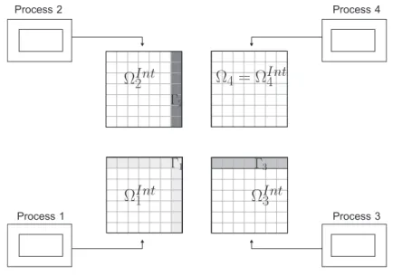
We use distributed memory model, so the matrixAis distributed among the processes and, as we use PETSc, the rows corresponding to the elements of each subdomain, including interior and local interfaces, reside in the same process, see Figure 3 for a four domain representation.

4.1 Preconditioner Setup

Algorithm 1 describes the construction of the fine and coarse components of the preconditioner.

Figure 3: Subdomain and matrix distribution among processes.

Algorithm 1: Preconditioner Setup

Input:A,kInt,kBord,kProd

Output:eLJ,UeJ,CeJ,BeJ,LSeJ,USeJ,LC,UC

Fine Component

1: [eLJ,UeJ] =ILU(AJJ,kInt), J=1, . . . ,P;

2: CeJ=IFS(eLJ,AJΓ,kBorder), J=1, . . . ,P;

3: BeJ=

IFS(UeT

J,ATΓJ,kBorder) T

, J=1, . . . ,P;

4: Se=AΓΓ−

P

∑

J=1

IP(BeJ,CeJ,kProd)

5: SeJ=RJSRe TJ, J=1, . . . ,P;

6: [L_eS

J,USeJ] =ILU(SeJ,kΓ), J=1, . . . ,P;

Coarse Component

7. [LC,UC] =LU(R0ART0).

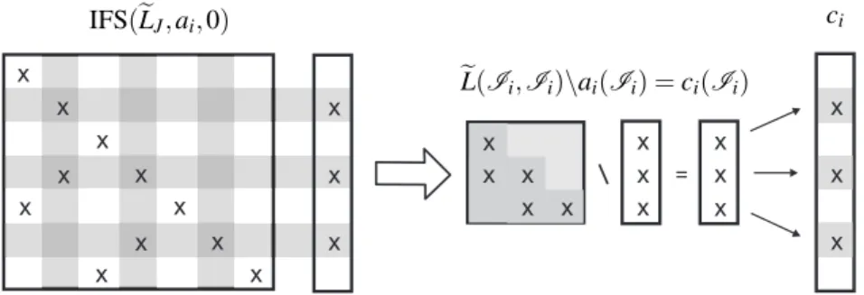
In Step 2,CeJ=IFS(eLJ,AJΓ,0)computes an approximationCeJ=eL−1AJΓ through a level zero

incomplete triangular solver applied to the columns ofAJΓ. For each columnaiofAJΓ, we take

I_{i, the set of indices of the nonzero elements ofai. Then we solveci(}I_{i) =}e_L(I_i,I_i)\ai(I_i),

light gray rows and columns represent theI_{i indices applied to the rows and columns of the} matrixeLJand the dark gray elements are the ones ineL(Ii,Ii). We use a PETSc routine to get

the submatriceseL(I_i,I_{i)as a small dense matrix and use our own dense triangular solver to} compute ci(Ii), which is a small dense vector, and then use another PETSc routine to store it

in the correct positions of ci, which is a column of the sparse matrixCeJ. We observe that the

nonzero columns ofAJΓthat take part in these operations, in each subdomain, are related to the

extended interface, but are stored locally.

IFS(eLJ,ai,0)

e

L(I_i,I_i)\ai(I_{i) =ci(}I_i)

ci

Figure 4: Incomplete Forward Substitution.

Note that eLJ andAJΓ (see Equation (2.5)) are in processJ, as can be seen in Figure 3, which

means that Step 2 is done locally without any communication.

Step 3 computes BeJ also through the incomplete forward substitution using the same idea

de-scribed for Step 2 , butAΓJ is not stored entirely in processJ. Actually,AΓJ has nonzero

ele-ments in the rows associated with the extended interfaceΓ_J, therefore the elements ofAΓJ are

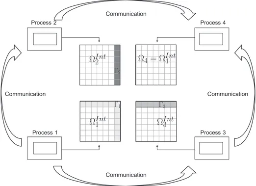
distributed among processJand its neighbors. So each process has to communicate only with its own neighbors to computeBeJ. The matrixBeJis stored locally in process J.

The communication layout of Step 3 is illustrated in an example for four subdomains in Figure 5, where the arrows show the data transfer flow. In this example, using, for instance, five-point centered finite differences, each subdomain has at most two neighbors, but in different 2-D or 3-D grids and with different discretization schemes, each subdomain can have more neighbors.

The Step 4 computes the Schur complement through an incomplete product as described by equa-tion (3.9). The submatrixAΓΓis formed by the subdomains interfaces and therefore is distributed

among the processes. Each process computes locally its contribution IP(BeJ,CeJ,kProd) and

sub-tracts globally fromAΓΓto build upSe, which is also distributed among the processes in the same

wayAΓΓ is. Again, each subdomain communicates with their neighbors following the pattern

illustrated in Figure 5, but with arrows pointers reversed, and there is a synchronization barrier to form the global matrixSe.

In Step 5 and 6, each process takes a copy of the local part ofSerelative to the extended interface

Figure 5: Domain distribution among processes.

In Step 7 the matrixR0ART0 is initially formed as a parallel matrix, distributed among the

pro-cesses. Local copies of this matrix is made in all processes and then a LU factorization is done redundantly. The order of this matrix isP, which is in general quite small.

4.2 Preconditioner Application

Algorithm 2 describes the application of the preconditionerMto the vectorr, i.e., the computa-tion ofz=Mr. We define two additional restriction operators,RΩJ :Ω→Ω

Int

J andRΓ:Ω→Γ.

These restriction operators are needed to operate on the correct entries of the vector, it can be seen as a subset of indices in the implementation.

Step 1 of Algorithm 2 solves a triangular linear system in each process involving theeLJ factor

and the local interior portion of the residual, obtainingzJ. This process is done locally and no

communication is necessary because the residualris distributed among the processes following the same parallel layout of the matrix.

Step 2 appliesBeJ multiplyingzJ and subtracting fromrΓobtainingzΓand the communication

between the neighbor subdomains is necessary only inrΓandzΓbecauseBeJ is stored locally in

process J.

The Schur complement application is done in Step 3. Because each process has a local copy of its parts ofSefactored intoL_SeeU_eS, only the communication inzΓbetween the neighbor subdomains

Algorithm 2: Preconditioner Application

Here we adopt the Matlab-style notationA\bto denote the exact solution ofAx=b. Input:r,eLJ,UeJ,CeJ,BeJ,LSeJ,USeJ,LC,UC

Output:z

1: zJ=eLJ\(RΩJr), J=1, . . . ,P;

2: zΓ=RΓr−

P

∑

J=1 e

BJzJ

3: zΓ=

P

∑

J=1 TJ

U_Se

J\

L_Se

J\(RJzΓ)

;

4: zJ=UeJ\

zJ−CeJzΓ

, J=1, . . . ,P;

5: zF=RTΓzΓ+

P

∑

J=1 RT_Ω

JzJ

Coarse correction:

6. z=zF+RT0(UC\(LC\R0r)).

which is applied through an element wise product. The result is then summed globally inzΓ. At

this point there is a synchronization barrier among all processes.

In Step 4 we apply theUeJ factor tozJ−CeJzΓ. The matrix-vector productCeJzΓrequires

com-munication among neighbors in zΓ and then the triangular solver is done locally with no

communication.

The vectors zJ and the vector zΓ are gathered in zF in Step 5, where zF is the residual

preconditioned by the fine component of the preconditioner.

Step 6 applies the coarse component, completing the computation of the preconditioned residual. Triangular solvers involved are local because there are local copies ofLCandUCin each process,

so no communication is necessary.

5 COMPARISON TESTS

We use two metrics to evaluate the preconditioners: the number of iterations and the solution time. In this section we describe the platform where the tests were run, present the results of the proposed preconditioner, and compare with a native PETSc preconditioner.

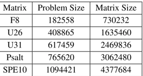
model. The fifth matrix is the standard SPE10 model [10] with over a million active cells. All the problems are black oil models using fully implicit method and there are four degrees of freedom per grid cell.

Table 1 shows the problems’ size considering the total number of cells and the size of their respective matrices.

Table 1: Test case problems.

Matrix Problem Size Matrix Size

F8 182558 730232

U26 408865 1635460 U31 617459 2469836 Psalt 765620 3062480 SPE10 1094421 4377684

For both preconditioners the problem was solved using native PETSc right preconditioned GM-RES method [27], with relative residual tolerance of 1e-4, maximum number of iterations of 1000, and restarting at every 30thiteration. The mesh was partitioned using PT-Scotch [9]. IS-chur has fill-in level 1 in the interior of the subdomains and zero in the interfaces, namelykInt=1, kBord=kProd=kΓ=0, as this specific configuration presented a better behavior in preliminary

Matlab tests.

We compare the proposed two-level preconditioner with PETSc’s native block Jacobi precondi-tioner (see [3]) combined (as in equation (3.1)) with the same coarse component presented in this paper. We refer to this combination simply as block Jacobi. We note that block-Jacobi/ILU is the default preconditioner in PETSc and is a common choice of preconditioner in reservoir simulation, which makes it an appropriate benchmark.

The first set of tests was run on an Intel Xeon(R) 64-bit CPU E5-2650 v2 @ 2.60GHz with 16 cores (hyper-threading disabled), 20MB LLC, 64GB RAM (ECC enabled). The operating system is a Debian GNU/Linux distribution running kernel version 3.2.65. The compiler is Intel Parallel Studio XE 2015.3.187 Cluster Edition.

The iSchur preconditioner, both in setup and application phases, requires more computation and communication than block Jacobi, so it has to present a pronounced reduction in number of iterations compared with block Jacobi in order to be competitive. Table 2 shows the number of iterations and the total time, in seconds, for both preconditioners, for all the tested problems, ranging from one to sixteen processes. For each test, the best results are highlighted in gray. We can observe that the iSchur preconditioner does reduce the number of iterations compared to block Jacobi for all problems in any number of processes. For one process (sequential execution), both preconditioners are equal, as there are no interface points, so we show the results just for the sake of measuring speed up and scalability. In average, iSchur does 80% as many iterations as block Jacobi. In this set of experiments, iSchur was more robust than block Jacobi, as the latter failed to converge in two experiments.

the size of the subdomains decreases. A correlated fact occurs with iSchur. In this case as we are using different levels of fill in the interface related parts and in the interior parts, more information is neglected with more subdomains, as the number of interface points increases.

Table 2: Number of iterations and the total time for both preconditioners from 1 to 16 processes. (NC) stands for “not converged”.

Mat Prec Number of Iterations Processes Total Time (s) Processes

1 2 4 8 16 1 2 4 8 16

F8 iS 104 113 106 92 102 10.8 7.9 4.1 2.1 1.8

bJ 119 109 125 135 6.1 3.0 1.9 1.7

U26 iS 92 131 199 218 303 22.0 19.8 14.5 9.1 9.9

bJ 252 NC 404 349 28.2 NC 13.3 9.7

U31 iS 69 110 449 517 864 28.0 28.8 48.7 32.1 43.1

bJ 124 593 639 NC 24.1 56.7 35.4 NC

Psalt iS 34 68 57 72 54 17.8 24.3 11.9 8.2 5.6

bJ 87 76 117 76 19.7 9.2 8.0 5.0

SPE10 iS 116 135 148 148 176 71.5 53.9 30.9 18.0 17.5 bJ 142 149 164 198 43.6 24.1 15.4 16.1

Table 2 also shows the total time of the solution using both preconditioners. We can see that despite the reduction in the number of iterations the solver time of iSchur is smaller than block Jacobi only in a few cases. One of the main reasons is that the iSchur setup time is greater than block Jacobi’s, especially when running on few processes. Although iSchur’s setup is intrinsi-cally more expensive than block Jacobi’s, we believe that this part of our code can still be further optimized to reduce this gap.

In reservoir simulation, the sparsity pattern of the Jacobian matrix only changes when the oper-ating conditions of the wells change, and therefore it remains the same over the course of many nonlinear iterations. This is an opportunity to spare some computational effort in the setup phase, since in this case the symbolic factorization does not need to be redone. We can see in Table 3 the time comparison when the symbolic factorization is not considered; in this scenario iSchur is faster in most cases. Furthermore, block Jacobi is a highly optimized, mature code (the default PETSc preconditioner), while iSchur could possibly be further optimized.

Table 3: Time of iterative solver without the symbolic factorization.

Iterative Solver Time (s)

Mat Prec Processes

1 2 4 8 16

F8 iS 10.5 6.3 3.3 1.7 1.6

bJ 6.1 3.0 1.9 1.7

U26 iS 21.7 16.2 12.7 8.2 9.4

bJ 28.1 NC 13.3 9.7

U31 iS 27.5 22.8 45.6 30.5 42.2 bJ 23.9 56.7 35.3 NC

Psalt iS 17.3 17.5 8.4 6.4 4.6

bJ 19.6 9.2 8.0 5.0

SPE10 iS 70.8 44.2 26.0 15.5 16.1 bJ 43.4 24.0 15.3 16.1

1 2 4 8 16 32 64 128 256 512

Processes

50 100 150 200 250

Ite

ra

ti

on

s

Psalt ischur Psalt bjacobi

SPE10 ischur SPE10 bjacobi

Figure 6: Comparison between block Jacobi and iSchur up to 512 processes.

6 CONCLUSIONS AND REMARKS

The scalability of both preconditioners is an on-going research as tests in a larger cluster are still necessary, but these initial results indicate a little advantage to iSchur.

For the current implementation the total solution time, setup and iterative solver, of the iSchur is smaller in only a few cases, where one important factor is the inefficiency in the setup step. The block Jacobi in PETSc is highly optimized while our implementation has room for improvement.

Removing the symbolic factorization time, considering the case when it is done once and used multiple times, which is usual in reservoir simulation, the solution using the iSchur precondi-tioner is faster for most tested cases. It shows that the presented precondiprecondi-tioner can be a better alternative than block Jacobi for the finer component when using two-level preconditioners to solve large-scale reservoir simulation problems. Furthermore, we deem that the application part of the code can still be optimized.

RESUMO. Discutimos a implementac¸˜ao paralela de um precondicionador alg´ebrico de decomposic¸˜ao de dom´ınios em dois n´ıveis baseado em ILU(k), utilizando a biblioteca PETSc. Apresentamos estrat´egias para melhorar a performance, minimizando a comunica-c¸˜ao entre processos durante as fases de construcomunica-c¸˜ao e de aplicacomunica-c¸˜ao. Comparamos, na solucomunica-c¸˜ao de sistemas lineares provenientes de problemas de simulac¸˜ao de reservat´orios, a nossa implementac¸˜ao com um precondicionador padr˜ao do PETSc. Mostramos que, para alguns casos, nossa implementac¸˜ao apresenta um desempenho superior.

Palavras-chave: Precondicionador de dois n´ıveis, decomposic¸˜ao de dom´ınio, m´etodos de Krylov, sistemas lineares, paralelismo, PETSc.

REFERENCES

[1] T. M. Al-Shaalan, H. Klie, A.H. Dogru, & M. F. Wheeler. Studies of robust two stage preconditioners for the solution of fullyimplicit multiphase flow problems. InSPE Reservoir Simulation Symposium, 2-4 February, The Woodlands, Texas, number SPE-118722 in MS, (2009).

[2] D. A. Augusto, L. M. Carvalho, P. Goldfeld, I. C. L. Nievinski, J.R.P. Rodrigues, & M.Souza. An algebraic ILU(k) based two-level domain decomposition preconditioner. InProceeding Series of the Brazilian Society of Computational and Applied Mathematics,3(2015), 010093–1– 010093–7. [3] S. Balay, S. Abhyankar, M. F. Adams, J. Brown, P. Brune, K. Buschelman, L. Dalcin, V. Eijkhout, W.

D. Gropp, D. Kaushik, M. G. Knepley, L. C. McInnes, K. Rupp, B.F. Smith, S. Zampini, H. Zhang, & H. Zhang. PETSc users manual. Technical Report ANL-95/11 - Revision 3.7, Argonne National Laboratory, (2016).

[4] M. Bollh¨ofer & V. Mehrmann. Algebraic multilevel methods and sparse approximate inverses.SIAM Journal on Matrix Analysis and Applications,24(1) (2002), 191–218.

[5] X. Cai & M. Sarkis. A Restricted Additive Schwarz Preconditioner for General Sparse Linear Systems SIAM Journal on Scientific Computing,21(2) (1999), 792–797.

[7] L. M. Carvalho, L. Giraud & P. L. Tallec. Algebraic two-level preconditioners for the Schur complement method,SIAM Journal on Scientific Computing,22(6) (2001), 1987–2005.

[8] T. F. Chan, J. Xu & L. Zikatanov. An agglomeration multigrid method for unstructured grids. Contemporary Mathematics,218(1998), 67–81.

[9] C. Chevalier & F. Pellegrini. PT-Scotch: A tool for efficient parallel graph orderingParallel computing, 34(6) (2008), 318–331.

[10] M. A. Christie & M. J. Blunt. Tenth SPE comparative solution project: A comparison of upscaling techniques in SPE Reservoir Simulation Symposium, (2001).

[11] D. A. Collins, J.E. Grabenstetter & P. H. Sammon. A Shared-Memory Parallel Black-Oil Simulator with a Parallel ILU Linear Solver. SPE-79713-MS. InSPE Reservoir Simulation Symposium, Houston, 2003. Society of Petroleum Engineers.

[12] L. Formaggia & M. Sala.Parallel Computational Fluids Dynamics. Practice and Theory., chapter Algebraic coarse grid operators for domain decomposition based preconditioners. Elsevier, (2002), 119–126.

[13] S. Gries, K. St¨uben, G. L. Brown, D. Chen & D. A. Collinns. Preconditioning for efficiently applying algebraic multigrid in fully implicit reservoir simulations.SPE Journal,19(04): 726–736, August 2014. SPE-163608-PA.

[14] H. Jackson, M. Taroni & D. Ponting. A two-level variant of additive Schwarz preconditioning for use in reservoir simulation.arXiv preprint arXiv:1401.7227, (2014).

[15] P. Jenny, S. Lee & H. Tchelepi. Multi-scale finite-volume method for elliptic problems in subsurface flow simulation.Journal of Computational Physics,187(1) (2003), 47– 67.

[16] P. Jenny, S. Lee & H. Tchelepi. Adaptive fully implicit scale finite-volume method for multi-phase flow and transport in heterogeneous porous media.Journal of Computational Physics,217(2) (2006), 627–641.

[17] P. Jenny, S. H. Lee & H. A. Tchelepi. Adaptive multiscale finite-volume method for multiphase flow and transport in porous media.Multiscale Modeling & Simulation,3(1) (2005), 50–64.

[18] A. Manea, J. Sewall & H. Tchelepi. Parallel multiscale linear solver for reservoir simulation. Lecture Notes - slides - 4th SESAAI Annual Meeting Nov 5, 2013, (2013).

[19] A. Muresan & Y. Notay. Analysis of aggregation-based multigrid. SIAM Journal on Scientific Computing,30(2) (2008), 1082–1103.

[20] R. Nabben & C. Vuik. A comparison of deflation and coarse grid correction applied to porous media flow.SIAM J. Numer. Anal.,42(2004), 1631–1647.

[21] F. Nataf, H. Xiang & V. Dolean. A two level domain decomposition preconditioner based on local Dirichlet-to-Neumann maps.Comptes Rendus Mathematique,348(21-22) (2010), 1163–1167. [22] Y. Notay. Algebraic multigrid and algebraic multilevel methods: a theoretical comparison.Numer.

[23] Y. Notay. Algebraic analysis of two-grid methods: The nonsymmetric case.Numerical Linear Algebra with Applications,17(1) (2010), 73–96.

[24] D. W. Peaceman Fundamentals of Numerical Reservoir Simulation.Elsevier, (1977).

[25] A. Quarteroni & A. Valli.Applied and Industrial Mathematics: Venice - 1, 1989, chapter Theory and Application of Steklov-Poincar´e Operators For Boundary-Value Problems. Kluwer, (1991), 179–203.

[26] Y. Saad.Iterative Methods for Sparse Linear Systems. SIAM, 2nd edition, (2003).

[27] Y. Saad & M. H. Schultz. GMRES: A generalized minimal residual algorithm for solving nonsymmetric linear systems SIAM Journal on scientific and statistical computing, 7(3) (1986), 856–869.

[28] Y. Saad & J. Zhang. BILUM: Block versions of multielimination and multilevel ILU preconditioner for general sparse linear systems.SIAM Journal on Scientific Computing,20(6) (1999), 2103–2121. [29] B. Smith, P. Bjørstad & W. Gropp.Domain Decomposition, Parallel Multilevel Methods for Elliptic

Partial Differential Equations. Cambridge University Press, New York, 1st edition, (1996).

[30] J. Tang, R. Nabben, C. Vuik & Y. Erlangga. Theoretical and numerical comparison of various pro-jection methods derived from deflation, domain decomposition and multigrid methods. Reports of the Department of Applied Mathematical Analysis 07-04, Delft University of Technology, January 2007.

[31] U. Trottenberg, C. Oosterlee & A. Schuller.Multigrid. Academic Press, Inc. Orlando, USA, (2001).

[32] C. Vuik & J. Frank. Coarse grid acceleration of a parallel block preconditioner.Future Generation Computer Systems, JUN,17(8) (2001), 933–940.