Technology and the changing family: a unified model of marriage, divorce, educational attainment and married female labor-Force participation

DISCUSSION PAPER SERIES

Forschungsinstitut zur Zukunft der Arbeit Institute for the Study of Labor

Technology and the Changing Family: A Unified Model

of Marriage, Divorce, Educational Attainment and

Married Female Labor-Force Participation

IZA DP No. 8831 February 2015 Jeremy Greenwood Nezih Guner Georgi Kocharkov Cezar Santos

Technology and the Changing Family:

A Unified Model of Marriage, Divorce,

Educational Attainment and Married

Female Labor-Force Participation

Jeremy Greenwood

University of Pennsylvania

Nezih Guner

ICREA-MOVE, Universitat Autonoma de Barcelona, Barcelona GSE and IZA

Georgi Kocharkov

University of Konstanz

Cezar Santos

Getulio Vargas Foundation

Discussion Paper No. 8831

February 2015

Any opinions expressed here are those of the author(s) and not those of IZA. Research published in this series may include views on policy, but the institute itself takes no institutional policy positions. The IZA research network is committed to the IZA Guiding Principles of Research Integrity.

The Institute for the Study of Labor (IZA) in Bonn is a local and virtual international research center and a place of communication between science, politics and business. IZA is an independent nonprofit organization supported by Deutsche Post Foundation. The center is associated with the University of Bonn and offers a stimulating research environment through its international network, workshops and conferences, data service, project support, research visits and doctoral program. IZA engages in (i) original and internationally competitive research in all fields of labor economics, (ii) development of policy concepts, and (iii) dissemination of research results and concepts to the interested public. IZA Discussion Papers often represent preliminary work and are circulated to encourage discussion. Citation of such a paper should account for its provisional character. A revised version may be available directly from the author.

IZA Discussion Paper No. 8831 February 2015

ABSTRACT

Technology and the Changing Family: A Unified Model of

Marriage, Divorce, Educational Attainment and

Married Female Labor-Force Participation

Marriage has declined since 1960, with the drop being bigger for non-college educated individuals versus college educated ones. Divorce has increased, more so for the non-college educated. Additionally, positive assortative mating has risen. Income inequality among households has also widened. A unified model of marriage, divorce, educational attainment and married female labor-force participation is developed and estimated to fit the postwar U.S. data. Two underlying driving forces are considered: technological progress in the household sector and shifts in the wage structure. The analysis emphasizes the joint role that educational attainment, married female labor-force participation, and assortative mating play in determining income inequality.

JEL Classification: E13, J12, J22, O11

Keywords: assortative mating, education, married female labor supply, household production, marriage and divorce, inequality

Corresponding author: Nezih Guner

MOVE (Markets, Organizations and Votes in Economics) Facultat d’Economia, Universitat Autònoma de Barcelona Edifici B – Campus de Bellaterra

08193 Bellaterra (Cerdanyola del Vallès) Spain

1

Introduction

The character of American households has changed dramatically since World War II. First, the number of married households has plunged, both due to a rise in the number of never-married households and an increase in the rate of divorce. The change has been most notable for non-college educated households. Second, there has been a rise in assortative mating. That is, people are more likely to marry someone of the same educational level today than in the past. Third, the fraction of college educated females and males has increased substantially. This is especially true for women. Fourth, there has been a dramatic rise in labor-force participation by married females. Fifth, income inequality across households has

widened signi…cantly.1

The goal of this paper is to develop a uni…ed theory capable of explaining this array of facts. The model has three key ingredients. First, marriage and divorce decisions are formalized within the context of a search-theoretic paradigm. People match randomly and only marry if both parties agree. A divorce occurs when one party in a marriage favors single life over married life. A divorcee is free to remarry if the opportunity arises. The attractiveness of a mate depends on his/her ability and educational level, as well as on the love arising from the relationship. Second, all individuals make a choice about whether to go college. They do this based on their ability and their psychic cost of going to school. Third, married households must decide whether the female should work. This depends on the wage women will earn in the market and the cost incurred by the household when she works. Labor at home is used in household production.

There are two exogenous driving forces in the analysis: Technological progress in the home and shifts in the wage structure. Technological progress in the home reduces the labor needed in household production. This makes it easier for married women to work in the market. Moreover, with better technology in the home, the economies of scale associated with married life matter less. Hence, this force promotes a decline in marriage and an increase in divorce. Two shifts in wage structure are entertained: an increase in the return to education and a decline in the gender wage gap. A rise in the return to education entices

more men and women to go to college. Shrinkage in the gender wage gap encourages labor-force participation by married women and makes singlehood more a¤ordable for females.

The framework developed connects the induced shifts in the structure of households to the rise in income inequality. As a thought experiment, suppose that husbands and wives work full time and that there is no gender gap. Then, random matching would reduce household income inequality. For this e¤ect to be operational, though, married women must work. Now, an increase in positive assortative mating works to amplify income inequality. This e¤ect will be stronger if women at the upper end of the income distribution work more than those at the lower end.

The uni…ed framework developed here is matched with U.S. data from the 1960s using a minimum distance estimation strategy. The procedure targets a collection of stylized facts concerning educational attainment, marriage and divorce, and married female labor-force participation. The framework …ts the data for 1960 well. The structural parameter values obtained also look reasonable, and are tightly estimated. The model predictions for 2005 are then compared with the corresponding U.S. data. A slight retuning of a very limited number of parameters is then undertaken before the framework is used to decompose the shift in family structure into its underlying driving forces.

Both driving forces are quantitatively important for explaining the changes in family structure outlined above. The …ndings suggest that technological progress in the household sector accounts for the majority of the rise in married female labor-force participation. The narrowing of the gender gap in wages plays a secondary role here, too. Technological progress in the household sector also has a conspicuous e¤ect in explaining the fall in marriage and the rise in divorce. Changes in the structure of wages are important for the increase in assortative mating and educational attainment.

While the rise in the skill (college) premium is the root cause for widening household income inequality, shifts in family structure provide a very important ampli…cation mecha-nism. An increase in the return to education entices more people in the right-hand side of the ability distribution to go to college, which makes household incomes more disperse. A rise in positive assortative mating implies that a high (low) earning woman is more likely to be matched in marriage with a high (low) earning man and this, too, heightens inequality. For

this latter e¤ect to be operational, however, married women must work in the labor force. Hence, the rise in married female labor-force participation also plays a role in generating household income inequality.

After a brief literature review in Section 1.1, the remainder of this paper is organized as follows: Section 2 describes the main facts in detail. The model is presented in Section 3. Section 4 discusses the calibration/estimation procedure for 1960 and then Section 5 con-siders the model results for 2005. Section 6 decomposes the e¤ects of each of the exogenous forces at play. Section 7 discusses the implications of the developed framework for household income inequality. Some concluding remarks are o¤ered in Section 8.

1.1

Relationship to the Literature

The framework developed here resembles, in some aspects, Greenwood and Guner (2009) who study the fall in marriage and the rise in divorce. However, their model does not have heterogeneity with respect to education and ability. By adding this in the current framework, it is possible to study implications regarding assortative mating and inequality. Another related paper is by Regalia and Ríos-Rull (2001), which was ahead of its time. While their model does feature heterogeneity in both females and males, the focus is on accounting for the rise in the number of single mothers, something left out of the current analysis. They stress market forces, such as a movement in the gender gap, as explaining this rise, but a mechanism for studying the rise in assortative mating appears to be absent. Jacquemet and Robin (2012) estimate a search and matching model of the marriage market for the U.S. Their analysis focuses on how female and male wages a¤ect marriage probabilities and the share of the marital surplus received by partners. Given this goal, there is no need to include endogenous divorce or educational attainment in their model, which is central to the current paper. Eckstein and Lifshitz (2011) study the e¤ect that di¤erent mechanisms (schooling, the gender wage gap, fertility, and marriage and divorce) had on the rise in the female labor-force participation during the twentieth century. They …nd that up to 42% of the change is left unexplained. They attribute this residual component to improvements in household technology and changes in social norms. This is consistent with the story told in this paper.

Parts of the picture have been addressed before elsewhere. Greenwood, Seshadri and Yorukoglu (2005) analyze the importance of technological progress in the home sector for

making it more feasible for married females to enter into the labor market.2 _{However, they}

do not study the changes in household structure or inequality, as done here. The interaction between inequality and positive assortative mating has also been noted by Fernandez and Rogerson (2001) and Fernandez, Guner and Knowles (2005). Chiappori, Iyigun and Weiss (2009) discuss how positive assortative mating provides a marriage market return for female educational investment, in addition to the traditional labor market one. The same e¤ect is at play in the model developed here and, together with the rise in married female labor-force participation, is important to explain the rise in household income inequality. Greenwood, Guner, Kocharkov and Santos (2014) document the rise in assortative mating in the U.S. between 1960 and 2005 and assess how much it contributed to the rise in inequality. They do this within a simple model-free accounting framework, while the emphasis here is on decomposing the endogenous household decisions in a structural model.

Di¤erent ways in which marriage and female labor supply decisions interact in the current framework have been pointed out in the literature. Neeman, Newman and Olivetti (2008), for example, argue that college-educated working females can a¤ord to be more selective in the marriage market and this may lead to more stable marriages. Such outside option e¤ect is also operational in the current framework. Gihleb and Lifshitz (2013) document that a married female who is more educated than her husband is more likely to work. They analyze how changes in assortative mating can account for shifts in married female labor supply. Here, both assortative mating and female market participation are also endogenously determined. This is done within an equilibrium framework that can be used to study income inequality.

2 _{Independent empirical work by Cavalcanti and Tavares (2008) and Coen-Pirani, Leon, and Lugauer}

(2010) also suggests that labor-saving household products have increased married female labor supply. Adamopoulou (2010) shows that they also have contributed to the rise of cohabitation. Advances in maternal medicine and pediatric care played a similar role, as has been noted by Albanesi and Olivetti (2015).

2

Facts

The shape of the American household has changed dramatically over the last 50 years. Some salient features of this transformation are:

1. The Decline in Marriage. The fraction of the population that has ever been married has fallen dramatically since 1960. At that time, about 85 percent of college educated individuals and 92 percent of non-college educated ones between the ages of 25 and 54 were married (or had been married)–see Figure 1. (Data sources for this and all other

…gures are provided in the Appendix.) Today, only 81 (79) percent are.3 _{Note that the}

fall in the fraction of the population that is married is greatest for non-college educated people. Part of the decline in marriage is due to a delay in the age of marriage. Part is due to a rise in divorce. In 1960 the fraction of the population that was divorced, as measured by the ratio of the currently divorced to the ever-married population, was 5 percent for the non-college educated populace and 3 percent for the college educated segment. Today, it is around 20 percent for the former and 12 percent for the latter. Again, observe that divorce has risen more for the non-college educated vis-à-vis the college educated. The fact that the decline in marriage and the rise in divorce has a¤ected college educated and non-college educated people di¤erentially has been noted both by sociologists, Martin (2006), and economists, Stevenson and Wolfers (2007). 2. The Rise in Assortative Mating. When individuals marry today, as opposed to

yester-day, they are more likely to pair with an individual from the same socioeconomic class. To see this split the world into two socioeconomic classes, viz non-college educated and

college educated, and compare the two contingency tables contained in Table 1.4

3 _{Redoing Figure 1 with currently-married and currently-divorced individuals, as opposed to ever-married}

and ever-divorced ones, delivers very similar patterns.

4 _{Greenwood, Guner, Kocharkov and Santos (2014) use …ve educational classes. The results there parallel}

1960 1970 1980 1990 2000 2010 0.78 0.80 0.82 0.84 0.86 0.88 0.90 0.92 0.94 Ever M ar ried, fr act ion of wom en Year 0.04 0.06 0.08 0.10 0.12 0.14 0.16 0.18 0.20 Di vor ced and si ngl e, fr act ion of ever m ar ried Marriage, < college Marriage, college Divorce, < college Divorce, college

Figure 1: Marriage and Divorce by Education

Table 1: Assortative Mating, age 25-54

1960 2005

Husband Wife Husband Wife

< College College < College College

<College 0.855 (0.821) 0.023 (0.056) <College 0.545 (0.427) 0.108 (0.226)

College 0.082 (0.115) 0.041 (0.008) College 0.109 (0.227) 0.237 (0.120)

Statistics Measuring Assortative Mating

2 _{= 33; 451 obs = 195; 034} 2 _{= 77; 739 obs = 288; 423}

= 0:41 = 1:08 = 0:52 = 1:43

The number in a cell shows the fraction of all matches that occur in the speci…ed category. The …gure in parenthesis provides the fraction that would occur if matching occurred randomly. First, note that there is positive assortative mating. To see this, focus on the diagonal elements in the tables. These cells show the fraction of matches where husband and wife have the same educational levels. The di¤erence between the actual and random matches in these cells is always positive, re‡ecting positive

assorta-tive mating. The hypothesis of random matching is rejected by the 2 statistics.5 The

Pearson correlation coe¢ cient, , which measures the degree of association between

the female and male educational categories, is also always positive. Second, the extent of positive assortative mating has become stronger over time. This can be seen in a number of ways. Note that between 1960 and 2005 the di¤erences between the cells along the diagonals for the actual and random matrices increased. For each year take the ratio of the traces of the matrices for actual and random marriages. Denote this ratio by , which divides the actual concordant matches by the random concordant ones. The higher this number is the higher the degree of positive assortative mating. This ratio rises from 1.08 in 1960 to 1.43 in 2005. Additionally, the Pearson correlation coe¢ cient, , moves up from 0.41 to 0.52.

To further illustrate the rise in assortative mating, consider running a regression for married couples of the form

educationwt = + education h t + X y2Y t education h t dummyy;t +X y2Y

t dummyy;t+ "t; with "t N (0; t);

(1)

where: educationw

t 2 f0; 1g is the observed level of the wife’s education in

pe-riod t and takes value of one if the woman completed college and a value of zero

otherwise; educationht 2 f0; 1g is the husband’s education; dummyy;t is a dummy

variable for time such that dummyy;t = 1 if y = t and dummyy;t = 0 if y 6= t;

t = 1960; 1970; 1980; 1990; 2000; _{and 2005 gives the years in the sample and Y is the}

subset of these years that omits 1960. The coe¢ cient t measures the additional

im-pact relative to 1960 that a husband’s education will have on his wife’s. Note that the impact of a secular rise in female educational attainment is controlled by the presence

of the time dummy variable. So, how does t change over time? Figure 2 plots the

5 _The 2_{statistics is calculated as}Pc i=1

Pr j=1

(Oi;j Ei;j)2

Ei;j ; where Oi;j and Ei;jare observed and expected

0.04 0.08 0.12 0.16 0.20 Regr essi on coef fici ent , γ t Year, t 1970 1980 1990 2000 2005 γ_t 95% bounds

Figure 2: Rise in Assortative Mating. The solid line plots the regression coe¢ cient, _t. The

dashed lines show the 95 percent intervals.

rise in the ts. The t coe¢ cients are signi…cantly di¤erent from one another at the

95 percent con…dence level. The same …nding obtains if instead logits or probits are run. The rise in assortative mating has been noted before by sociologists Schwartz and

Mare (2005).6

3. The Increase in Education and Labor-Force Participation by Females. Labor-force

participation by married females has increased dramatically over the last 50 years.7

This is true for both college educated and non-college educated women. In 1960 a minority of both classes of women worked. Now, the majority do–see Figure 3. At the same time, the number of women choosing to educate themselves has risen sharply. This may have been stimulated by a rise in the college premium, shown in Figure 4. College-educated women have always worked more than non-college educated ones. As female labor-force participation rose so did a married woman’s contribution to family income–again, see Figure 3. Figure 4 also shows how the gender wage gap has

6 _{Blossfeld and Timm (2003) document that the rise is not just a U.S. phenomenon but it is also observed}

in other developed countries.

7 _{Here, as discussed in Appendix 9.1, labor-force participation is taken as the fraction of women who}

work (employment rate). Taking into account the unemployed women in the labor-force only changes these statistics slightly.

1960 1970 1980 1990 2000 2010 0.3 0.4 0.5 0.6 0.7 0.8 Fem al e Labor -Force P ar tici pat ion Year College < College 1960 1970 1980 1990 2000 2010 0.10 0.15 0.20 0.25 0.30 Fr act ion Year Family Income

Figure 3: The Increase in Female Labor-Force Participation. The inset panel shows the contribution of married females to family income.

narrowed.

4. The Increase in Income Inequality. The distribution of income among households became more unequal between 1960 and 2005. The left-hand-side panel of Figure 5 shows the Lorenz curves for 1960 and 2005. Lorenz curves plot the cumulative share of income at each income percentile against the cumulative percentile of households. If income was equally distributed among households, these curves would coincide with the

450 _{line. The Lorenz curves show that the inequality increased. The Gini coe¢ cient,}

which is twice the area between the Lorenz curves and the 450 _{line, increased from 0.31}

to 0.43 between 1960 and 2005. Another way to see this is by plotting the household income relative to the mean household income in each percentile; this is done in the right-hand side of Figure 5. The relative income for all households below the 80th percentile declined, while there was a signi…cant increase for households who are at the top of the income distribution.

1950 1960 1970 1980 1990 2000 2010 5 10 15 20 25 30 Year C ol lege D egr ee, % of fem al es 1960 1970 1980 1990 2000 2010 1.4 1.5 1.6 1.7 1.8 1.9 2.0 2.1 C ol lege P rem ium Gap Premium 0.40 0.45 0.50 0.55 0.60 0.65 G ender G ap

Figure 4: The Rise in Female Educational Attainment, the College Premium and the Nar-rowing of the Gender Gap

0.0 0.2 0.4 0.6 0.8 1.0 0.0 0.2 0.4 0.6 0.8 1.0 C um ul at ive S har e of H ousehol d Incom e

Cumulative Percentile of Households

2005 1960 gini2005 = 0.429 gini1960 = 0.306 0.0 0.2 0.4 0.6 0.8 1.0 0.0 0.5 1.0 1.5 2.0 2.5 3.0 H ousehol d Incom e R el at ive to M ean Percentile 2005 1960

3

Model

What are the economic forces behind this dramatic shift in household characteristics? The idea can be described in a nutshell. People marry for both economic and noneconomic reasons: material well-being and love. On the material side of things, a woman’s labor is important for both home production and market production. Over time the value of a woman’s labor in home production has declined, due to technological progress in the household sector. Speci…cally, inputs into home production, such as dishwashers, frozen foods, microwave ovens, washing machines, and most recently the internet, have reduced the

need for household labor.8 _{At the same time, the value of a woman’s time in the market and}

her incentives to obtain additional education increased as a result of a narrower gender wage gap and a higher skill premium. Therefore, love and the value of a woman’s labor on the market have come to play more important roles, relative to the value of a woman’s labor in home production, in the decision about whether or not to get married and whom to marry. A rise in the skill premium heightens income inequality. If more high ability people go to college (relative to low ability ones), then the earnings di¤erential between high and low ability individuals will widen. A higher skill premium creates a greater incentive to match assortatively. So, changes in marriage patterns can intensify inequality. But, for this mechanism to have force, married women must work in the market. Otherwise, if women never worked, household income inequality would closely follow the inequality among men.

To formalize the discussion above four things are required. First, a model of marriage and divorce is needed. Second, the framework must include a decision about whether or not married females should work. Third, the structure should incorporate an education decision. Fourth, people must be heterogenous in ability. This motivates the following setup.

8 _{While the focus here is on marriages, these forces reduce the need to live in large households in general.}

Bethencourt and Ríos-Rull (2009) and Salcedo, Schoellman and Tertilt (2012) model the rise in single families, but in contexts not involving marriage. In a similar vein, Greenwood and Guner (2009) model the decisions of young people to leave their parent’s home.

3.1

Setup

Imagine an economy that is populated by equal numbers of females, f , and males, m. Some females and males are college educated, while others are non-college educated. Some individuals of each gender will be married, the rest either divorced or never married. A

person faces a constant probability of dying, , each period. Upon death an individual is

replaced by a young doppelganger who is about to begin his or her adult life. A person enters adult life with an ability level a 2 A. Initial ability is distributed across the population in line with the distribution function A(a). It will be assumed that a is log normally distributed

so that ln a N (0; 2

a), where 2a denotes the variance of this zero-mean distribution.

The …rst decision that a young adult makes is whether or not to acquire an education.

An uneducated male will earn the amount w0a for each unit of labor supplied on the market,

while an educated one earns w1a, where w1 > w0. A female earns the fraction 2 [0; 1] of

what a comparable male does. This re‡ects the gender gap in labor income. Acquiring an education has an up-front utility cost . For a person of gender g 2 ff; mg with ability a;

is a random variable drawn from the distribution Cg

a( ). Assume that Cag( )is a normal

distribution with mean _g=a and variance 2_{. The idea here is that the cost of learning}

is inversely related to a person’s ability, so on average higher ability individuals have lower costs of education. There is, however, mixing, since even among individuals with high ability there will be some who draw a high cost of education. Let e 2 E =f0; 1g represent whether (e = 1) or not (e = 0) a person has acquired an education. After the education decision,

each individual will be characterized by an ability level, a, and education level, e.9 _Denote

a person’s type by (a; e) 2 T A E.

Skill-biased technological progress results in skilled labor becoming more valuable relative

to unskilled labor. Therefore, w1 will grow over time relative to w0 and the college premium

moves up. As a consequence, more males will complete college. More females should …nish college too. Take a single female …rst. The income earned when single will now have risen for a college educated woman, relative to a non-college educated one. Thus, a college educated single female can now live better than before (again, relative to an non-college educated one).

9 _{It is optimal for an individual to get education in the …rst period. There is only a one-time utility cost}

The extra income that a college education now provides means that a college educated single woman can a¤ord to be choosier when selecting a husband. The same reasoning applies to being single because of a divorce.

Now, consider a married female. If she works, the return to a college education will have risen because her family will have more income (assuming that married women work). This provides an incentive to become more educated. This fact will also make a college educated woman more attractive on the marriage market. The return from …nding a better partner on the marriage market, in and of itself, may provide an extra return for females (and males) to invest in college. A decline in the gender gap (a rise in ) will reinforce women’s incentives to acquire a college education. These forces should cause people to become pickier about their mate, causing a decline in marriage and a rise in divorce. Educated individuals are also less willing to marry uneducated agents, as with a higher skill premium, the cost of marrying an uneducated person is higher. Hence, one would expect a rise in assortative mating. This mechanism intensi…es the e¤ect of a step up in the skill premium on income inequality.

At the beginning of each period people must decide whether or not to work in the market during the period. Each person has one unit of time per period, which can be used for market

or home production. Let hf and hm denote the hours worked by a female and a male in

the market, respectively. The workweek in the market is …xed. This is re‡ected in the two

possible values that h can take, h 2 H f0; hg. Suppose single agents always work full

time, allocating h to market and 1 h to household work. It is assumed that in marriage

h is chosen only for the wife; the husband always works full-time.10 _{Once a female decides}

whether or not to get educated at the start of her life, her wage rate does not change. In particular, females who choose to stay home do not experience any future wage penalty. The importance of labor market experience for the labor supply decisions of married females is emphasized, among others, by Eckstein and Wolpin (1989) and Eckstein and Lifshitz (2011). Olivetti (2006) documents an increase in the returns to experience for women and links it to the rise in their market participation. If experience matters for female wages, higher risk of divorce can encourage wives to work, as discussed by Fernandez and Wong (2014).

10 _{The e¤ect of changes in home technologies and wages on the time allocation decisions of husbands and}

Home goods are produced according to

n = d + (1 )(z hT)

1=

, 0 < < 1, (2)

where d is the amount of household durables, hT is the total amount of time spent on market

work, and z 2 f1; 2g is the household’s size. The restriction that 0 < < 1 implies that

household durables, d, and time, z hT, are substitutes in household production. Household

durables, d, can be purchased at the price p in terms of the market goods. The substitutability between labor and durable goods in household production implies that labor will be released from married households if the price of durables drops due to technological advance in the home sector. This promotes a rise in married female labor-force participation.

At the end of each period a single person will meet someone else of the opposite sex, with ability level a and education e . The couple will then draw two shocks. The …rst is a match-speci…c bliss shock b 2 B, taken from the distribution F (b). In particular, b

will be normally distributed so that b N (bs; 2b;s), where bs and 2b;s denote the mean

and variance of the bliss distribution that an unmarried couple draws from. In a marriage

the bliss shock evolves according to the distribution G(b0_{jb). Speci…cally, the bliss shock is}

assumed to follow the autoregressive process b0 _{= (1}

b;m)bm+ b;mb + b;m

p

1 _b;m", with

" N (0; 1). Here bm and 2b;m represent the long-run mean and variance of this process,

while _b;m is the coe¢ cient of autocorrelation. A married person will decide whether or not

to remain with their current partner partly on the value of this bliss shock.

The second shock, q 2 Q = fql; qhg, measures the cost for a married woman of going

to work.11 _{Without loss of generality, assume that q}

l < qh. Some families may place a

greater value on the woman staying at home; perhaps they are more likely to have children,

a factor abstracted away from here. The q shock is drawn from the distribution Qe;e (q),

which depends on the education levels of the husband, e, and wife, e . It is assumed that

Qe;e (q) is uniform and a matched couple draws ql and qh with equal probabilities. Finally,

it is assumed that Qe;e (q) depends only on the education level of the husband; i.e., there

is one distribution for couples with college-educated husbands and another one for couples

11 _{Guner, Kaygusuz and Ventura (2012) employ a similar strategy to model female labor-force}

with non-college educated husbands. This assumption is elaborated on further when the estimation strategy is discussed below. This shock is assumed to be permanent and hence

does not change over time.12 _{The couple then decides whether or not to marry. This}

decision will be based upon both economic and noneconomic considerations, as will soon become clear.

One barrier for married women going to work is the presence of young children. Modeling fertility endogenously is a substantial complication. The unitary model of the household must now be abandoned, because the presence of children a¤ects men and women di¤erently upon a divorce. Some form of a bargaining model must now be used— see Greenwood, Guner and Knowles (2003). As a practical matter, an accounting decomposition exercise along the lines of Greenwood, Guner, Kocharkov and Santos (2014) shows that changing fertility has little

impact on income inequality.13 _{Part of the cost of a married woman going to work might be}

child care costs, so q could partially re‡ect these. The e¤ect of these latter costs on married female labor supply is examined by Attanasio, Low and Sanchez-Marcos (2008).

The noneconomic factors underlying a marriage consist of the value of b, the value of q, and a measure of how compatible a couple is. For a couple with education levels e and e , this compatibility is represented by the function M (e; e ), where

M (e; e ) = ₀(1 e)(1 e ) + ₁(ee ):

If neither person went to college then this function returns a value of 0, since e = e = 0,

while if both are college educated then it gives a value of ₁. It yields 0 for all other cases.14

If these parameters do not change over time, then any changes in assortative mating over time will be generated endogenously by the model only in response to technological progress

in the household sector and to changes in the wage structure. Changes in ₀ and ₁;on the

other hand, can capture changes in assortative mating due to other factors, such as changing

12 _{It is assumed that this cost has no bite once a marriage is dissolved. As a result, and absent an explicit}

fertility decision or a cost of divorce, divorced and never-married females are indistinguishable in the model economy.

13 _{To be more precise, in such an accounting exercise, imposing the 1960 fertility patterns to the 2005}

economy only increases the Gini coe¢ cient from 0.430 to 0.434.

14 _{It could alternatively be assumed that a fraction of agents match within their own education group}

social norms in the marriage market.15 The economic factors are based upon each person’s ability and educational attainment; that is, their (a; e) pair.

Now, suppose married women stay at home when the skill premium rises. It is still possible for more women to go to college. The increased return to skill will entice more men to acquire a college education. The fact that there are more college educated men around implies that there may be a bigger incentive for women to invest in college education in order to become more desirable on the marriage market (because of compatibility considerations).

Last, let all people discount the future at the rate = e(1 ), where e is the subjective

discount factor. Suppose that for singles tastes over the consumption of market goods, c, and nonmarket ones, n, are represented by

Ts(c; n) = 1 1 (c c) 1 + 1 n 1 _;

wherec is a …xed cost in terms of market goods. Assume that in marriage the utility derived

from consumption and love is a public good. Momentary utility for a married household is

Tm(c; n) = 1 1 c c 1 + 1 + 1 n 1 + 1 ;

where < 1 is the adult equivalence scale. The equivalence scale re‡ects the fact that there

are economies of scale in household consumption, so that a two-person household requires less than the twice the consumption of a one-person household in order to realize the same

level of utility as the latter. The variablesc and provide an economic motive for marriage.

A two-person household will be better o¤ than single-person ones. As incomes grow over

time the …xed cost, c, will be easier to cover. Therefore, a trend to smaller households will

emerge. This will be re‡ected in a lower marriage rate and a higher divorce rate.

Now, suppose that > , which implies higher diminishing marginal utility for household

goods vis-à-vis market ones. In this case, single households will bene…t the most from technological advance in the home sector. This is because at the margin they will be the most intensive users of home production, as paradoxical as this may seem. That is, while the

15 _{Modeling changes in societal norms, a factor out of the purview of the current analysis, is the subject}

economically better o¤ married couple (due to economies of scale) will consume more of all goods, relative to a single person, they will not consume twice as much home goods, because they will prefer to direct, at the margin, their larger consumption bundle toward market ones. Technological progress in the home allows for more home goods to be produced. It will improve single life the most because the marginal value for a home produced good is highest for singles. This operates to reduce household size over time.

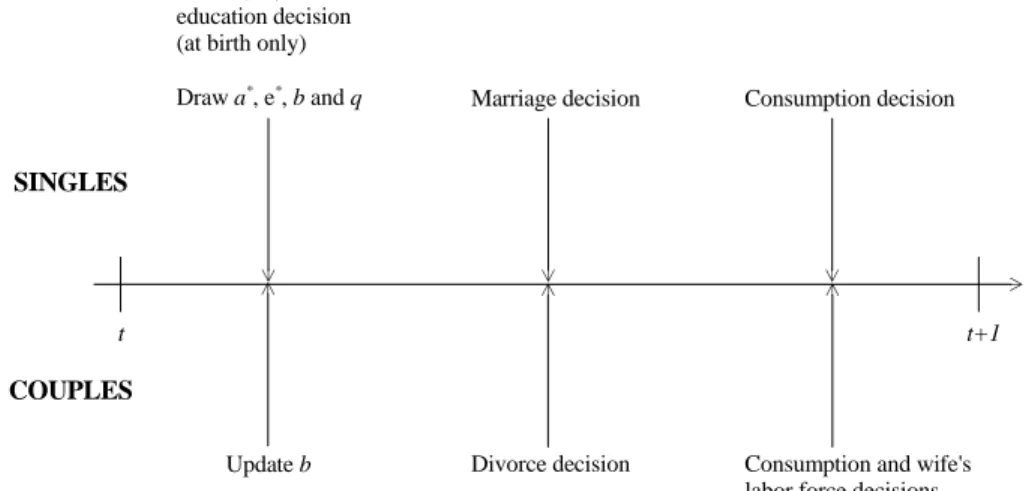
To complete the description of the setting, the timing of events within a period is il-lustrated in Figure 6. At any point, the model economy will be populated by married, single-male and single-female households. Some of these married households will have hus-bands and wives who are college educated, while others will have two non-college educated members, and yet others will have a college educated husband and a non-college educated wife or vice versa. Similarly, single households will also di¤er by their educational attain-ments. Furthermore, not all educated agents will have the same earnings, since they have di¤erent ability levels. Finally, some married females will participate in the labor market while others won’t. These di¤erences will generate inequality among households, and the model economy provides a natural framework to study how changes in household structure a¤ect inequality.

3.2

Singles

Consider the consumption decision facing a single. This is a purely static problem. For a single person of gender g 2 ff; mg with ability a and educational attainment e 2 f0; 1g, the problem is given by U_sg(a; e) max c;n;dTs(c; n); (3) subject to c = 8 < : we ah pd; if g = f; weah pd; if g = m; and n = d + (1 )(1 h) 1= .

t t+1

SINGLES

Draw a, κ, and make education decision (at birth only) Draw a*

, e* , b and q

COUPLES

Marriage decision Consumption decision

Divorce decision

Update b Consumption and wife's

labor force decisions

with ability a and educational attainment e. Suppose that this individual meets someone of the opposite gender, g , who has ability a and education attainment e and the potential

couple draws shocks b and q. Will they get married? To answer this question, let Vg

s(a; e)

and Vsg (a ; e ) represent the expected lifetime utilities that both parties will realize if they

remain single in the current period. Likewise, denote the expected lifetime utility that is

associated with a marriage in the current period by Vg

m(a; e; a ; e ; b; q). A marriage will

occur if and only if

V_mg(a; e; a ; e ; b; q) V_sg(a; e) and V_mg (a ; e ; a; e; b; q) V_sg (a ; e ): (4)

Observe that for a marriage to happen it must be the …rst choice for both parties. Let the

indicator function 1g_{(a; e; a ; e ; b; q) take a value of 1 if both people in the match want it}

and value of zero otherwise. Thus,

1g(a; e; a ; e ; b; q) = 8 < : 1; if (4) holds, 0; otherwise. (5)

[Observe that 1g_{(a; e; a ; e ; b; q) = 1}g _{(a ; e ; a; e; b; q).]}

The value of being single in the current period will depend on the distribution of potential future mates on the marriage market. Each mate is indexed by their (a ; e ) combination.

Let the distribution of potential mates from the opposite gender be represented by bSg _{(a ; e ).}

This will be elaborated on later. The value function for a single person of gender g with ability a and educational attainment e can now be expressed as

V_sg(a; e) = U_sg(a; e) (6) + Z Q Z B Z T f1g(a; e; a ; e ; b; q)V_mg(a; e; a ; e ; b; q)

+[1 1g(a; e; a ; e ; b; q)]V_sg(a; e)_gdbSg (a ; e )dF (b)dQe;e (q), for g = f; m:

Embedded in the above dynamic programming problem is the assumption that one will draw a mate next period with an ability level less than a and education level e with probability

b

Sg (a ; e ).16

3.3

Couples

The static consumption problem for a married couple is

U_mg(a; e; a ; e ; q) max c;n;d;hf_2f0;1gTm(c; n) h f q; (7) subject to c = 8 < : we a h + we ahhf pd; if g = f; weah + we a hhf pd; if g = m; and n = d + (1 )(2 h hhf) 1= :

Recall that all utility ‡ows are public goods within a marriage. So, the couple picks c; n; d,

and hf together. Working in the market takes away the fraction h of a person’s time

endowment. Recall that husbands are assumed to work full-time. The variable hf

2 f0; 1g represents the wife’s participation decision. It takes a value of 1 when the woman works and a value of 0 if she doesn’t. Once again, the variable q gives the cost for a married woman of going to work. This is netted out of household utility, when the woman works. Let

Hf_{(a; e; a ; e ; q)}

2 f0; 1g denote the female labor force participation decision for a couple of type (a; e; a ; e ; q):

A divorce will occur if and only if

V_sg(a; e) V_mg(a; e; a ; e ; b; q) or V_sg (a ; e ) V_mg (a ; e ; a; e; b; q): (8)

Therefore, the indicator function 1g_{(a; e; a ; e ; b; q), speci…ed by (5), will return a value of}

one if both the husband and wife want to remain married and will give a value of zero if one

16 _{Other matching processes could be envisaged, such as the Gale and Shapley algorithm employed by Del}

of them desires a divorce. Given this, the value function for a married person reads

V_mg(a; e; a ; e ; b; q) = U_mg(a; e; a ; e ; q) + b + M (e; e ) (9)

+ _f

Z

B

[1g(a; e; a ; e ; b0; q)V_mg(a; e; a ; e ; b0; q)

+[1 1g(a; e; a ; e ; b0; q)]V_sg(a; e)]dG(b0_{jb)g, for g = f; m:}

This value function is used in equations (4), (5), (6) and (8); likewise, (6) is employed in (4), (5), (8) and (9).

3.4

Educational Choice

People choose their education level at the beginning of adult life after they observe ; the

utility cost of education. The problem they face is max

e2f0;1gfV g

s(a; e) e g; (10)

where Vg

s is de…ned by (6). The decision rule stemming from this problem will be represented

by a simple threshold rule, since Vg

s(a; 1) > Vsg(a; 0); E_ag( ) = 8 < : 1 if _eg_a; 0 if >_eg_a: (11)

The total number of agents of gender g with ability a who choose to get a college degree is

then given by _Z

1 1

E_ag( )dC_ag( );

and the total number of gender g agents with college education is

Z 1

0

Z 1

1

3.5

Steady-State Equilibrium

The dynamic programming problem for a single person, or (6), depends upon knowing the solution to the problem for a married person, as given by (9), and vice versa. Furthermore, to solve the single’s problem requires knowing the steady-state distribution of potential mates

in the marriage market, Sg_{(a). The non-normalized steady-state distribution for singles is}

Sg(a0; e0) = (1 ) Z Q Z B Z a0_;e0 T Z T

[1 1g(a; e; a ; e ; b; q)]dSg(a; e)dbSg (a ; e )dF (b)dQe;e (q)

+(1 ) Z Q Z B Z B Z a0_;e0 T Z T [1 1g(a; e; a ; e ; b; q)]dMg(a; e; a ; e ; b 1; q)dG(bjb 1) + e0 Z ₁ 1 E_ag0( )dC g a0( )dA(a0) + (1 e0) 1 Z ₁ 1 E_ag0( )dC g a0( )dA(a0) for g = f; m: (12)

In the above recursion, Mg_{(a; e; a ; e ; b}

1; q) represents the steady-state distribution over

married people and bSg (a ; e )denotes the normalized distribution for singles of the opposite

gender and is de…ned by

b Sg (a ; e ) S g _{(a ; e )} R T dS g _{(a ; e )}: (13)

The …rst term in (12) counts those singles who failed to match in the current period. The second term enumerates the ‡ow into the pool of singles from failed marriages. The last two terms represent the arrival of new adults (the doppelgangers).

In similar fashion, the distribution of married men and women is de…ned by

Mg(a0; e0; a 0; e 0; b0; q0) = (1 ) Z q0 Q Z b0 B Z a0_;e0 T Z a 0_;e 0 T 1g(a; e; a ; e ; b; q)

dbSg (a ; e )dSg(a; e)dF (b)dQe;e (q)

+(1 ) Z q0 Q Z b0 B Z B Z a0_;e0 T Z a 0_;e 0 T 1g(a; e; a ; e ; b; q) dMg(a; e; a ; e ; b 1; q)dG(bjb 1), for g = f; m: (14)

The …rst term on the right-hand side measures the ‡ow into marriage from single life. Only

num-ber of marriages that will survive from the current period into the next one. To com-pute a steady-state solution for the model amounts to solving a …xed-point problem, as the

following de…nition of equilibrium should make clear. [Note that Mg_{(a; e; a ; e ; b}

1; q) =

Mg (a ; e ; a; e; b 1; q).]

De…nition 1 A stationary matching equilibrium is a set of value functions for singles and

marrieds, Vsg(a; e) and Vmg(a; e; a ; e ; b; q), an education decision rule for singles, Eag( ), a

matching rule for singles and married couples, 1g_{(a; e; a ; e ; b; q), and stationary}

distribu-tions for singles and married couples, Sg_{(a; e) and M}g_{(a; e; a ; e ; b}

1; q), all for g = f; m,

such that:

1. The value function Vg

s(a; e) solves the single’s recursion (6), taking as given her/his

indirect utility function, Ug

s(a; e), from problem (3), the value function for a married

person, Vg

m(a; e; a ; e ; b; q), the matching rule for singles, 1g(a; e; a ; e ; b; q), and the

normalized distribution for singles, bSg(a; e), de…ned by (13).

2. The value function Vmg(a; e; a ; e ; b; q) solves a married person’s recursion (9),

tak-ing as given her/his indirect utility function, Ug

m(a; e; a ; e ; q), from problem (7), the

matching rule for a married couple, 1g_{(a; e; a ; e ; b}0_{; q), and the value function for a}

single, Vsg(a; e).

3. The decision rule Eg

a( ) solves a single’s education problem (10), taking as given

Vg

s(a; e) from (6).

4. The matching rule 1g(a; e; a ; e ; b; q) is determined in line with (5), taking as given

the value functions Vg

s(a; e) and Vmg(a; e; a ; e ; b; q).

5. The stationary distributions Sg_{(a; e) and M}g_{(a; e; a ; e ; b}

1; q) solve (12) and (14),

taking as given the decision rule for an education, Eag( ), and the matching rule

4

Fitting the Model to the U.S. in 1960

The model developed will now be …t to the U.S. data for 1960. There are many parameters. A few of them are easy to choose and can be assigned on the basis of a priori information. Most of the parameters will be …tted using a minimum distance estimation procedure, however. The estimation procedure will focus on the 1960 U.S. economy. In the next section the model will be simulated using 2005 wages and durable goods prices and the resulting …t examined. It will be assumed that the model is in a steady state for each of these years.

4.1

A Priori Information

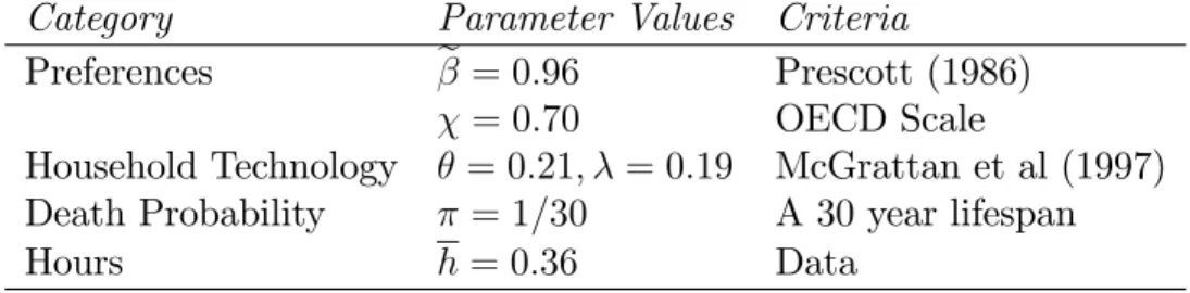
The easy ones are done …rst. The length of period is one year. Let e (the subjective discount factor) be 0.96, a standard value in macroeconomic studies, such as in Prescott (1986). All the targets for the estimation are calculated for individuals between ages 25

and 54, which corresponds to an operational lifespan of 30 years. Set = 1=30 = 0:033 so

that individuals in the model also live 30 years on average. This would dictate a value for

the discount factor of = 0:960 (1 0:033). Assigning a value for the work week, h, is

straightforward. Assume a 40 hour work week. Since there are 112 non-sleeping hours in a

week, let h = 40=112 = 0:36.17 _{Last, the household production parameters, and , have}

been estimated by McGrattan, Rogerson and Wright (1997). Their numbers, = 0:21 and

= 0:19; are used here.18 _{Finally, in line with the OECD equivalence scale, set = 0:70.}

To summarize, the parameter values picked on the basis of a priori information are displayed in Table 2.

17 _{An alternative would be to set h to actual hours worked per week. The value of h would then be}

0.37, 0.35, and 0.39 in 1960 for single males, single females, and married males, respectively, and 0.38, 0.36, and 0.40 in 2005. Simulating the model economy for 1960 and 2005 with these values, instead of h = 0:36, produces almost identical results.

18 _{The parameter determines the elasticity of substitution between durable goods and household time,}

1=(1 ). McGrattan, Rogerson and Wright (1997) identify this parameter using time series variation. Since targets from a single year (speci…cally, 1960) are used to estimate the parameters here, is not included among them. Table B1 in Appendix B shows the 1960 model statistics when is increased or decreased by 20%, while all other parameters are kept at their benchmark values. Changes in do not have any major e¤ect on 1960 targets.

Table 2: Parameters –A Priori information

Category Parameter Values Criteria

Preferences e = 0:96 Prescott (1986)

= 0:70 OECD Scale

Household Technology = 0:21; = 0:19 McGrattan et al (1997)

Death Probability = 1=30 A 30 year lifespan

Hours h = 0:36 Data

4.2

Minimum Distance Estimation

This leaves 23 parameters to be assigned. There are 6 preference parameters, f ; c; ; ; 0; 1g;

5 parameters for the marital bliss shocks, fbs; b;s; bm; b;m; b;mg; 3 wage parameters fw0;1960; w1;1960; 1960g;

1 parameter for durable goods prices, p1960;3 parameters for the cost of education, f f; m; g;

and 1 parameter for the ability distribution, a: It is assumed that qh and ql di¤er by the

education level of the husband. Let q1

h and ql1 denote the cost of joint work for couples with

a college educated husband, and qh0 and ql0 be the corresponding values for households with a

non-college educated husband. This adds 4 more parameters. For both types of husbands, it is assumed that there is an equal chance of drawing a high or a low cost. Normalize the wage

rate for a non-college educated male in 1960 to be one, so that w0;1960 = 1: The remaining

22 parameters are estimated so that the model matches, as closely as is possible, a set of 25

data moments for 1960.19

The data targets are:

1. Educational Attainment. The fraction of females and males that went to college. 2. Vital Statistics. The fraction of the population that has ever-been married by

edu-cational level, and that is currently divorced (out of the ever-married populace) by

education level.20

19 _{In the data used, observations come from a mixture of di¤erent cohorts. In the model, there is}

es-sentially an in…nite horizon cohort, with some of its members dying each period and being replaced with doppelgangers. One way to get the data to be close to the steady state approximation is to use averages of a sub-period rather than just a single year. The decennial census that is used to compute the moments contains data for 1960 only. Computing the same data targets using the Current Population Survey (CPS) for several years in the 1960s (1962-1965) yields remarkably similar statistics.

3. Assortative Mating. A contingency table for marriage that contains the fractions of marriages for each possible combination of educational levels for both the husband and wife.

4. Married Female Labor-Force Participation. The fraction of married females, classi…ed by the education levels of husbands and wives, that work, and the share of household income provided by wives.

5. Skill premium and gender earnings gap: The earnings ratio between college educated and non-college educated males (the skill premium), and the earnings ratio between females and males (the gender gap).

6. Inequality: The Gini coe¢ cient for earnings inequality among households; the 90-to-10 and 90-to-50 percentile ratios; income inequality across married households by the educational attainments of husbands and wives; and the ratio of single female to married household income.

Before the parameter estimates and the model …t are presented, a comment on the skill premium and gender wage gap as targets is in order. Take the skill premium …rst. Wages

are needed for non-college and college educated males in 1960; viz, w0;1960 and w1;1960. Recall

that w0;1960 = 1. The college premium in 1960 for the model is the average ratio of earnings

for a college educated male to a non-college educated one, as given by w1;1960 hR1 0 R1 1aE m a ( )dCam( )dA(a) i =hR₀1R1₁E_am( )dC_am( )dA(a)i hR1 0 R1 1a(1 Eam( ))dCam( )dA(a) i =hR₀1R1₁(1 Em a ( ))dCam( )dA(a) i:

This is an endogenous variable, because young single males decide whether or not to go to

and consumption. Hence, it is a model of couples living together rather than being legally married. While it is possible to combine the married and cohabiting population to arrive at a stock of people who live together, it is more problematic to calculate a separation rate for cohabiting people. In the U.S. Census the divorced category only covers those who had been married in the past. See Gemici and Laufer (2014) for a study of cohabitation and marriage. These authors calculate dissolution rates for married and cohabiting couples from the Panel Study of Income Dynamics. The calculation of such rates, however, is only possible after 1978.

school. The strategy here is to pin down w1;1960;along with other parameters, such that this

statistic is as close as possible to its data counterpart, about 1.55 in 1960.

A similar strategy is followed to determine the gender wage gap parameter 1960: Recall

that Mf_{(a; e; a ; e ; b; q)and S}f_{(a; e)are non-normalized distributions of married and single}

females, respectively. As in the data, average earnings for females are calculated for those who work; i.e., all singles and married ones who participate in the labor market. This is given by

1960w1;1960

Z :::

Z

aeHf(a; e; a ; e ; q)dMf(a; e; a ; e ; b; q)

+ ₁₉₆₀

Z :::

Z

a(1 e)Hf(a; e; a ; e ; q)dMf(a; e; a ; e ; b; q)

+ ₁₉₆₀w1;1960

Z Z

aedSf(a; e) + ₁₉₆₀

Z Z

a(1 e)dSf(a; e):

(Again, w0;1960 = 1.) The …rst and second terms in this equation give the average earnings

for married skilled and unskilled women who decide to work. The last two terms calculate the same statistic for single women. On the other hand, since all males, single or married, work, the average earnings for them read

w1;1960 Z ₁ 0 Z ₁ 1 aE_am( )dC_am( )dA(a) + Z ₁ 0 Z ₁ 1 a(1 E_am( ))dC_am( )dA(a) :

The gender earnings gap in the model is the ratio of these two averages. The parameter

1960 is estimated, again along with other parameters, to generate a gender earnings gap in

the model that is as close as possible to the observed gender earnings gap in the data, about 0.45 in 1960.

Let data represent a vector of 25 moments that are calculated from the U.S. data for 1960. A vector of the analogous 25 moments can be obtained from the steady state of the model for 1960. The results for the model will be a function of the parameters to be estimated, of course. Therefore, represent this vector of moments by M(!) where ! denotes the vector of 22 parameters to be estimated. De…ne the vector of deviations between the

data and the model by G(!) _{data M(!).}

Minimum distance estimation picks the parameter vector, !, to minimize a weighted sum of the squared deviations between the data and the model. Speci…cally,

b

! = arg min G(!)0W G(!);

where W is some positive semi-de…nite matrix. The estimation assumes that the model is a true description of the world, for some value of the parameter vector, !. The number of

targets is larger than the number of parameters. The estimator, !, is consistent for any_b

weighting matrix, W . Let se(!)_b represent the vector of standard errors for the estimator,!._b

It is given by

se(!) = diag_{b f}[J (!)b

0_{W J (!)]b} 1_{J (!)b} 0_{W W J (!)[J (b !)b} 0_{W J (!)]b} 10

n g;

where J (_b!) @_M(b!)=@!,_b is the variance-covariance matrix for the data moments, and

n is the total number of observations.21 The data moments are calculated from the 1960

U.S. Census. Each element in is weighted by the number of observations for a particular

moment relative to the total number of observations. Set W = I, where I is the identity matrix.

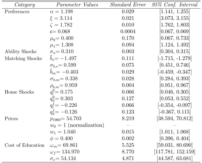
Table 3 reports the parameter estimates and their associated standard errors. The set of moments and the corresponding results for the benchmark model for 1960 are displayed in Table 4. The …tted parameter values look reasonable and are tightly estimated, for the most part.

21 _{Each diagonal element of corresponds to the variance of a particular moment in the data. Since most}

Table 3: Parameters –Estimated (Minimum Distance)

Category Parameter Values Standard Error 95% Conf. Interval

Preferences = 1:198 0.029 [1.141, 1.255] = 3:114 0.021 [3.073, 3.155] = 1:782 0.010 [1.762, 1.803] c= 0:068 0.0004 [0.067, 0.069] 0= 0:400 0.170 [0.067, 0.733] 1= 1:308 0.094 [1.124, 1.492] Ability Shocks a= 0:310 0.003 [0.304, 0.315] Matching Shocks bs= 1:497 0.111 [-1.715, -1.279] b;s= 0:599 0.075 [0.451, 0.746] bm= 0:403 0.029 [-0.459, -0.347] b;m= 0:338 0.028 [0.284, 0.393] b;m= 0:959 0.004 [0.951, 0.967] Home Shocks q0_l= 0:175 0.066 [0.046, 0.305] q0 h= 0:303 0.127 [0.053, 0.552] q1 l= 0:226 0.066 [-0.354, -0.097] q1_h= 0:126 0.123 [-0.367, 0.115] Prices p1960= 54:703 8.219 [38.594, 70.812] w0 = 1 (normalization) – – w1 = 1:040 0.015 [1.011, 1.068] = 0:400 0.002 [0.396, 0.404] Cost of Education !m= 69:861 5.525 [59.031, 80.690] !f= 134:970 8.770 [117.781, 152.159] e= 54:134 4.871 [44.587, 63.681]

The estimate of the degree of curvature in the utility function for market goods ( = 1:78) is in line with the macroeconomics literature, which typically uses a coe¢ cient of

relative aversion of either 1 or 2. Note that nonmarket goods have a weight of = 1:20in

utility. This can be thought of as corresponding to a weight assigned to consumption in a typical macro model of 0:45, with the remaining weight of 0:55 being applied to leisure; i.e., 0:55=0:45 = 1:20. Nonmarket goods play a role similar to leisure here. Thus, this coe¢ cient does not seem unreasonable. The utility function for nonmarket goods is more concave ( = 3:114) than the one for market goods. As was mentioned in Section 3, this implies that a household will tilt its allocation towards market goods as it gets wealthier, and, as a result, this parameter a¤ects the di¤erences in marriage and divorce rates for educated and

non-educated individuals.

A household spends about 19 percent of its market consumption on covering the …xed

costs of a home (whenc = 0:068). This …xed cost provides an economic motive for marriage

since married agents can pool resources to cover c. It also gives an incentive for married

women to participate in the market. If c were set to zero, with all other parameters kept

at their benchmark values, the fraction of single individuals would be 20 percent (instead of 15 percent). Furthermore, married women are less likely to participate in the labor market. Married female labor-force participation would be only 3.5 percent. The parameters of the marital bliss shocks determine marriage and divorce rates in the model. Note that the

distribution for singles has a lower mean ( 1:497 versus 0:403), but a higher variance

(0:599 versus 0:338), than the one for married couples. This creates an incentive for singles to wait for a match with high b. Once a marriage is formed, marital bliss is quite persistent

( b;m = 0:959).22 An educated person realizes 1.308 utils ( 1) from marrying a similarly

educated person. The extra utility for a marriage between two non-educated individuals is lower, 0.4. These are higher than the mean level of bliss in a marriage of -0.403 and in‡uence

the level of marital sorting. Setting ₀ and ₁ to zero in the 1960 economy would generate

a correlation between husbands and wives education that is close to zero.

The estimation requires that joint work is costly for households in which the husband

is non-college educated (q0_l = 0:175 and q0_h = 0:303), but there is a bene…t of joint work

for households in which the husband is educated (q1

l = 0:226 and q1h = 0:126). Given

husband’s educational attainment, these parameters determine how the labor-force partic-ipation of a married female changes with her own education. This allows the benchmark economy to produce the observed response of female labor-force participation with respect to female educational attainment. Finally, the variance of the ability distribution, together with the parameters that determine the cost of education, weigh on both the fraction of individuals who choose to get a college education and the overall level of inequality.

22 _{In the simulations, N (b}

s; 2b;s) and b0= (1 b;m)bm+ b;mb + b;mp1 b;m" are approximated on a

discrete grid of size 15 using Tauchen’s (1986) procedure. Similarly, N (0; 2

a) is approximated on a grid of

As Table 4 illustrates, the model has no problem matching most of the targets. Single females relative to married couples are poorer in the model than they are in the data. The model misses the relative income of households that are composed of a college-educated wife and a non-college educated husbands. Note, however, that there is a very small number of such households (only 2.8 percent of all marriages). The model yields a slightly higher level of divorce in 1960; 3.3 percent in the data versus 4 percent in the model for college educated people and 5.3 percent in the data versus 4.4 percent in the model for non-college educated ones. As a result, the proportion of singles in the model is also higher than the data in 1960. The model has some di¢ culty mimicking the very high rate of marriage for the non-college educated in 1960.

Table 4: Data and Benchmark Model, 1960

Data Model

Education Fem Males Fem Males

0.072 0.125 0.074 0.129

Marriage

Fraction Sing Marr Sing Marr

0.130 0.870 0.151 0.849

Rates <Coll Coll <Coll Coll

–Marriage 0.925 0.849 0.888 0.882

–Divorce 0.053 0.033 0.044 0.040

Sorting Wife Wife

Husband

<Coll 0.855 0.023 0.843 0.028

Coll 0.082 0.040 0.085 0.045

Corr, educ 0.414 0.403

Work, Marr Fem

Husband Wife Wife

<Coll Coll <Coll Coll

<Coll 0.328 0.528 0.318 0.586 Coll 0.213 0.347 0.207 0.294 Participation, all 0.324 0.315 Income, frac 0.110 0.122 Inequality Gini 0.306 0.307 Ratio 90/10 4.829 4.536 Ratio 90/50 1.817 2.043 Income, Sf/M 0.543 0.393 Income, Marr

Husband Wife Wife

<Coll Coll <Coll Coll

<Coll 0.932 1.335 0.943 0.700

Coll 1.369 1.501 1.400 1.501

5

Moving Forward to 2005

The model economy is now ready to be simulated for 2005. This is done using the 2005 prices for durable goods and 2005 wages. As will be seen, in order the match the U.S. data as best as possible a very limited number of parameters need to be tweaked for 2005. These parameters involve the utility cost of education and compatibility between individuals of di¤erent education levels. There are two key goals of the analysis. The …rst is to assess the importance of the two driving forces for (i) the rise in assortative mating, (ii) the decline in marriage and the increase in divorce, which has impacted on non-college educated individuals more than college educated ones, (iii) the rise in educational attainments and married female labor-force participation, and (iv) increase in income inequality among households. This assessment is undertaken in Section 6. Before doing this, it is important for the model to match the U.S. data for 2005. The second goal is to understand the role that the change in family structure plays in generating income inequality. This is done is Section 7. Again, a good …t is desirable before pursuing this goal.

5.1

U.S. Stylized Facts and Benchmark Model Results

In order to simulate the model economy for 2005, …rst set w0;2005;the wage rate for unskilled

individuals, to 1:17, as the earnings of non-college educated males grew by 17 percent between

1960 and 2005. Next, w1;2005 (the wage rate for an e¢ ciency unit of skilled labor) and

2005 (the gender wage gap) are chosen such that the skill premium and the gender earnings

gap in the model economy are as close to their data counterparts as possible. The skill premium increased from 1.55 to 2.02 between 1960 and 2005. At the same time, women’s earnings relative to men’s increased from 0.45 to 0.64. Matching these two targets in 2005

implies w1;2005 = 1:81 (vs. w1;1960 = 1:04) and 2005 = 0:59 (vs. 1960 = 0:40).

Durable goods were also cheaper in 2005 than they were in 1960. Gordon (1990) reports that the quality-adjusted price of consumer durables declined between 6 percent and 13 per-cent a year for di¤erent durables between 1950 and 1985. A price index for eight durables (refrigerators, air conditioners, washing machines, clothes dryers, TV sets, dishwashers, mi-crowaves and VCRs) fell at 10 percent a year. In the National Income and Product Accounts,

the price index for “furnishings and durable household equipment”relative to the price index for “personal consumption expenditures” dropped by about 60 percent between 1960 and

2005 (close to 2 percent a year).23 _{In the simulation it will be assumed that the price of}

durables falls by 5 percent a year, a value between these two estimates. Consumer durable

goods prices in 2005 are then given by p2005 = p1960 e 0:05(2005 1960).24

Finally, _f and _m are allowed to take di¤erent values in 2005. (Recall that given a, an

individual of gender g draws , the utility cost of an education, from a normal distribution

with mean g=a and variance 2 ). The 2005 values for these parameters are selected such

that the model economy generates exactly the increase in educational attainment that is observed in the data. If these parameters are not allowed to change between 1960 and 2005, the model still generates an increase in the educational attainment, but the increase

is smaller, especially so for females.25 _{Matching the observed skill premium and the gender}

earnings gap in 2005 economy is possible, only if the model also delivers the correct levels of educational attainments men and women. In order to match the rise in educational

attainment, _f and _m had to be decreased from 134.97 to 69.6 and from 69.86 to 58.55

between the 1960 and 2005 steady states, respectively. The model requires a larger decline

in the cost of education for females.26 _{All other parameters are kept in their 1960 values.}27

23 _{Source: National Income and Product Accounts (NIPA), Table 2.3.4, Price Indexes for Personal}

Con-sumption Expenditures by Major Type of Product, version October 30, 2014.

24 _{The results for 2005 model economy with lower (2.5%) and higher (7.5%) price declines are reported}

in Table B2 in Appendix B. The decline in marriages and the rise in female labor-force participation are weaker (stronger) with a lower (higher) price decline.

25 _{Table B3 in Appendix B shows the 2005 model economy results when}

f and mare kept in their 1960

levels. The fraction of males and females who choose a college education would be 20.4 percent and 10.3 percent, respectively. For males, this is about 40 percent of the increase in educational attainment between 1960 and 2005. For females, however, the increase is much smaller. The educational attainment of females would only increase from 7.4 percent to 10.3 percent between 1960 and 2005, which is just 11 percent of observed rise.

26 _{Several changes that are not modeled here might be behind these exogenous shifts in education costs.}

For example: the federal government began guaranteeing student loans in 1965, which increased accessibility to colleges. Moreover, Title IX of the Education Amendments, passed in 1972, banned discrimination against women in education. Another factor might be changes in social norms, that are not explicitly modeled within the current framework.

27 _{It is assumed that the survival probability, , takes the same value in 1960 and 2005. Life}

ex-pectancy at birth increased by 7.7 years between 1960 and 2005 (The 2012 Statistical Abstracts of the US, Table 104. Expectation of Life at Birth, 1960 to 2008, and Projections, 2010 to 2020, available at http://www.census.gov/compendia/statab/cats/births_deaths_marriages_divorces/life_expectancy.html). Individuals enter the model economy, however, at age 25 and leave the model at age 55. As a result, the e¤ect of changes in life-expectancy for the model economy will be very small. Nevertheless, a counterfactual