Algorithmic composer, an unconventional music classification system

(1)

Master Program in Advanced Analytics

NOVA Information Management School

Instituto Superior de Estatística e Gestão da Informação Universidade Nova de Lisboa

Algorithmic Composer, an Unconventional

Music Classification System

Carolina Almeida Duarte

Dissertation submitted in partial fulfillment

of the requirements for the degree of

Master in Advanced Analytics

(2)

(3)

The Faculty of Sciences and Technology and the NOVA University Lisbon have the right, perpetual and without geographical boundaries, to file and publish this dis-sertation through printed copies reproduced on paper or on digital form, or by any other means known or that may be invented, and to disseminate through scientific repositories and admit its copying and distribution for non-commercial, educational

(4)

(5)

To all of those who supported me throughout this journey. Every second I shared with you was timeless. Your company has inspired me and made me a better person.

(6)

(7)

Acknowledgements

I would like to express my gratitude to my advisor Professor Leonardo Vanneschi, for his support in the development of this thesis and, specially, for his joy and dedication as a teacher which sparked my own passion for the Machine Learning world.

I would also like to thank Bea Babiak and András Kolbert, my dearest friends and colleagues during the first year of the Masters and from whom I have learned so much. Also, this thesis would not be possible without Miguel Domingos - you introduced me to Music. You have inspired me with your knowledge and with your skills.

And finally, I would like to thank my dearest work friends, with whom I have shared so much during the last year. I feel blessed to have met you all. Márcia Pinheiro, Sara Lopes, Joana Loureiro, Alexandra Jesus, Tiago Rodrigues... And especially you, André Marques! You gave me the strengh and energy to finish this document.

(8)

(9)

Abstract

Music is an inherent part of the human existence. As an art, it has mirrored its evolution and captured its thinking and creative process over the years. Given its importance and complexity, machine learning has long embraced the challenge of analyzing music, mainly through recommendation systems, classification and compo-sition tasks.

Current classification systems work on the base of feature extraction and analysis. The same applies for music classification algorithms, which require the formulation of characteristics of the songs. Such characteristics can be of varying degrees of complex-ity, from spectrogram analysis to simpler rhythmic and melodic features. However, finding characteristics to faithfully describe music is not only conceptually hard, but mainly too simplistic and restrictive given its complex nature.

A new methodology for music classification systems is proposed in this thesis, which aims to show that the knowledge learned by state of the art composition systems can be used for classification, without need for direct feature extraction.

Using an architecture of recurrent neural networks (RNN) and long-short term memory cells (LSTMs) for the composition systems and implementing a voting scheme between them, the classification accuracy of the experiments between classes of the Nottingham dataset ranged between 60% and 95%. These results provide strong evi-dence that composition systems do indeed possess valuable information to distinguish between classes of music. They also prove that an alternative method to standard classification is possible, as classification targets are not directly used for training.

Finally, the extent to which these results can be used for other applications is discussed, namely its added value to more complex classification systems, as well as to recommendation systems.

Keywords: Music Classification; Composition Systems; Recurrent Neural Networks; Long Short Term Memory Cells

(10)

(11)

Resumo

A Música é uma componente inerente à existência humana. Enquanto arte, tem refletido a sua evolução e captado o seu processo cognitivo e criativo ao longo dos tem-pos. Tendo em conta a sua importância e complexidade, a área do Machine Learning desde há muito abraçou este desafio, sobretudo através de sistemas de recomendação, classificação e composição musical.

Os sistemas de recomendação atuais funcionam na base de extração de features e respetiva análise. O mesmo se aplica a algoritmos de classificação musical, que re-querem a formulação de características musicais. Estas podem ter diferentes graus de complexidade, desde análise de espectros a simples features melódicas e rítmicas. Contudo, formular caracteríticas musicais não só é conceptualmente difícil, como so-bretudo simplista e restritivo dada a sua natureza complexa.

Uma nova metodologia para sistemas de classificação musical é proposta nesta tese, com o objectivo de demonstrar que o conhecimento aprendido por sistemas de composição pode ser utilizado para classificação, sem que haja necessidade de um processo de conceptualização e extração de características.

Utilizando uma arquitectura de redes neuronais recorrentes e células de memória longa e curta para os sistemas de composição e implementando um sistema de votação entre eles, a precisão para classificações binárias entre as classes do Nottingham dataset variou entre 60% e 95%. Estes resultados demonstram uma forte evidência de que os algoritmos de composição podem ser utilizados para tarefas de classificação e provam ainda que um método alternativo à classificação convencional é possível.

Finalmente, a aplicabilidade destes resultados para outros projetos é discutida, nomeadamente o valor acrescentado que pode trazer para sistemas de classificação mais complexos, assim como a sistemas de recomendação.

Palavras-chave: Classificação Musical; Sistemas de Composição; Redes Neurais Recor-rentes; Células de Memória Longa e Curta

(12)

(13)

List of Figures

3.1 Three Layer Neural Network. . . 9

3.2 The sigmoid activation function and its derivative. . . 11

3.3 Basic Structure of a Recurrent Neural Network. . . 15

3.4 Unfolded Recurrent Neural Network along the time axis. . . 15

3.5 Structure of a basic Neural Network cell. . . 16

3.6 Structure of a Long-Short Term Memory cell (LSTM).. . . 16

3.7 Forget Gate of a LSTM cell.. . . 17

3.8 Input Gate of a LSTM cell. . . 18

3.9 Output Gate of a LSTM cell. . . 18

5.1 Proposed Architecture of the Classification System.. . . 28

5.2 Sample Matrix with 15 time steps, 2 melody notes and 1 chord. . . 30

5.3 Note played within the limits of the defined time step. . . 33

5.4 Note played during the previous time step and also at the beggining of the current time step. . . 33

5.5 Note played at the end of the current time step and also in the following time step. . . 33

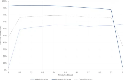
6.1 Accuracy of the notes and chords prediction for a varying melody coefficient. 41 6.2 Distribution of the chords and melody notes in the Nottingham dataset. . 42

(16)

(17)

List of Tables

6.1 Results obtained for the binary classification between the categories ”Hpps” and ”Waltzes”. . . 44

6.2 Results obtained for the binary classification experiments between the cat-egories ”Jigs”, ”Reels”, ”Hpps” and ”Waltzes”.. . . 44

6.3 Results obtained for the binary classification experiments between the cat-egories ”Reels” and ”Jigs”. . . 45

6.4 Results obtained for the binary classification experiments using a voting system between the categories ”Jigs”, ”Reels”, ”Hpps” and ”Waltzes”. . . 46

(18)

(19)

Chapter 1

Introduction

Machine learning techniques have opened new possibilities in a world where most seemed already explored. Wherever there is data, there is potential for discovery. There has come a time when it is possible to stare again at an immense ocean and wonder what is beyond. An ocean of data waiting to be uncovered.

Reality is data waiting to be processed and comprehended – it is why it is such a plentiful resource – and yet, some things are still hardly recognized as such because of their unstructured nature. Music, for instance. Music is the information the human mind extracts from a collection of sounds. However, thinking of music as data is still somehow surprising. The first goal of this thesis is therefore to explore a subject outside the beaten path and increase the sensibility and awareness of what data is and is not and how it can be treated in order to extract information from it.

With the current machine learning solutions, the number of tasks that only the human mind can do in comparison with intelligent systems is rapidly decreasing and in many cases the performance of the later has been higher than the former – otherwise, such systems would not be in use. Music, however, is still a task reserved to the talented mind. Intelligent systems are still far from composing at a high-quality level or even understanding music, mostly because of our inability to properly describe it so that the knowledge behind its creation can be learnt. This brings the second goal of this thesis – to explore the current work made on the field regarding music composition and classification and understand its fundamental ideas, as well as its weaknesses and strengths.

An investigation of the current state of music classification algorithms reveals an interesting paradox. Classification systems work based on characteristics of the data, from which several algorithms can be applied to determine a function that performs a better separation between classes. In the case of music classification systems, those characteristics are musical features of the songs. However, given the inherent difficulty of describing something as complex as music, it makes little sense to base a classifi-cation system on characteristics that are unable to capture the nature of music itself. This factor brings motivation and inspiration to the theme of this thesis, which is to

(20)

C H A P T E R 1 . I N T R O D U C T I O N

develop a new concept of a musical classification system that avoids the direct use of characteristics of the songs, requiring no extraction of the same.

Such system will be based on the performance of the composition systems on the songs to be classified. Each composer will be specialized in a certain class of music, which can theoretically be achieved by training it only with songs that belong to that class. It is then expected that, given a song, the composition system which better succeeds at predicting it will determine its class.

With this methodology, no direct training on the target variable is performed for the classification and no need for direct extraction of features of the songs is necessary, which represents a new paradigm in classification algorithms. In order explore this concept, the current work is organized as follows. In section 2 the literature of current composition and musical classification algorithms is reviewed. Section 3 provides basic knowledge on the mathematical foundations of the algorithms which will be used ahead. Section 4 explores a variety of musical representations and its weaknesses and strengths regarding its use for composition. In section 5, the structure and technical details of the classification system proposed in this thesis are explained in detail and in section 6 its results on several different experiments are presented and discussed. Finally, section 7 provides an overlook of future improvements to the current work, as well as perspective of its value and scope of application.

(21)

Chapter 2

Previous and Related Work

Music has long captivated and inspired the human mind, with millions of songs being composed over the course of history. What might be surprising at first sight is that music is also data – much like everything that surrounds us. To be aware of reality is to be cognizant of the surrounding events and this is only possible when receiving data from those elements – when the lights go off, awareness of the surrounding space is lost. Music is the brain’s interpretation of the information present in sound waves and so, in its simplest form, data waiting to be processed.

With music being such a plentiful and challenging type of data, and considering its importance to society, the research on the field has been intensive. The main fields of study include recommendation systems, classification and algorithmic composition. In this thesis, the focus will be on the latter two.

2.1 Algorithmic Composition

For years, music composition has been a task reserved only to the most talented. Time has brought new players into action and, since the 1950s, different computational techniques related to Artificial Intelligence have been used for composition. Hiller and Isaacson introduced the first computer-generated musical piece in 1955 [1]. The “lliac Suite” was a composition for string quartet divided into four experiments - the first three where generated with pre-defined musical rules and the fourth using variable order Markov chains. This work was particularly interesting as it contained the two main approaches later followed in the field: rule-based and learning systems.

Rule-based systems are the most intuitive means of creating an artificial compo-sition and rely on a set of rules which the computer is obliged to follow either in producing or assessing music. The complexity of such rules may vary, but a simple example may be found in the Musical Dice Games developed by Mozart in which pre-composed phrases were combined using a table of rules and the outcome of a dice roll. Those rules can also embody complex knowledge about specific musical styles, as in [18] where 270 production rules, constraints and heuristics where found from the

(22)

C H A P T E R 2 . P R E V I O U S A N D R E L AT E D WO R K

empirical observation of J. S. Bach chorales.

The systems previously described use rules to evaluate randomly generated se-quences of music and their connection with the previously defined sequence. How-ever, more complex systems can be built based on rules, as is the case of evolutionary algorithms. Such algorithms rely on a fitness function to evaluate sequences and then evolve them through a set of operators that simulate the effects of crossover and mu-tation on a population of musical sequences. In theory, human evaluation could be used to assess the quality of those sequences, however it is not a scalable solution. This fitness bottleneck can be eliminated by creating automated evaluators, which are commonly defined as a weighted sum of a set of features of the composition [9]. Rel-evant works can be found in [1], [7] and [21], where several rules concerning melody, harmony and rhythm are incorporated into a fitness function and in [11], where a statistical approach is taken to find mean values for certain characteristics, with fit-ness being then defined as the distance between the individual and the mean of the characteristic.

Two main issues arise with the rule-based systems described: not only it is difficult to determine rules concerning what is musically pleasant or not - whenever a set of rules is nailed down, exceptions and extensions are always discovered that necessitate more rules [3] - but those rules can also restrict the system. With music being an art, creativity and unpredictability are both critical. Rule-based systems, by definition, lack exactly this higher-level knowledge.

Learning systems are the other main approach to music composition - rather than requiring the development of a set of musical rules, they are trained on a set of musical examples. As such, and unlike rule-based systems, the richness of the final composi-tions is only limited by the power of the algorithm and, naturally, by the data itself. The first notable works following this approach used Markov chains [1] [2].

Although Markov-process music has proven to be successful over the short term, it has failed to show structure over the long term. In other words, the events at a given time have a small influence range over the following events, which for time dependent problems such as music is a critical downside. Theoretically this issue could be overcome by using higher order chains, for they would allow to increase the influence range along the time axis. However, this would imply an exponential growth in the state space, making it increasingly difficult to adequately populate the corresponding transition matrix and, ultimately, to train the model [4]. For this reason, recurrent neural networks (RNNs) have taken place as the number one choice for learning composition systems. In theory, their architecture should allow an easier exploration of long term dependencies on time series problems.

However, the first works on music composition with RNNs revealed difficulties in the training procedure, as stated by Mozer (1994) [5]. In his work, melodies were generated by a system named CONCERT, which was trained on sets of 10 Bach pieces to generate melodies by note-wise prediction. The results exposed a lack of ability

(23)

2 . 2 . C L A S S I F I C AT I O N

to learn the global structure of the music, similarly to what had been reported with Markov chains. But the issue was identified - the difficulty in training the system was due to the vanishing gradient problem.

The vanishing gradient problem, as described by Bengio et al. (1994) [32] causes difficulty in learning long term dependencies in the sequence. It is inherent not only to RNNs, but to all gradient based methods in general and may be avoided to some extent using different techniques. Regarding RNNs, the problem can be solved us-ing modified cells – Long-Short Term Memory cells (LSTMs). As the name suggests, each of these cells contains an internal memory that allows them to keep track of the information considered relevant, even if it refers to events from a distant past.

Several studies have been made in the recent years using this architecture (RNN + LSTM), for instance [24] and [31]. Mostly, they differ by the type of music

representa-tion used and the extent to which the different components of the music are used for prediction – if more than one instrument is used, if only chords or only melodies are predicted, etc. Regarding the representation of music, various alternatives have been studied, with focus on text and binary matrix representations. The first corresponds to music written in abc notation and can be viewed as a natural language processing (NPL) problem, as explored in [29] and [24]. This approach is certainly richer than a binary matrix representation, however it is also considerably slower to successfully train such systems. For this reason, and as composition is not the final goal of this thesis, a binary matrix representation is used.

Works following this approach can be found in [35], [31] and [15], with focus on the former two, for they successfully analyze both the melodic and the harmonic structure of music and thus serve as the main source of inspiration for the composition system used in this thesis.

2.2 Classification

Reality is a continuous flow of information – processing such an amount of data is a task the human mind has successfully accomplished through its ability of finding patterns and organize them into groups.

Algorithmic classification aims at automating this task and ultimately apply it to problems that are still unreachable. This process usually implies the identification of characteristics that are as unique as possible to the subject of study. Music clas-sification follows the same direction – clasclas-sification in genre / artist / epoch, etc. is usually accomplished by determining a set of characteristics and feeding them into an algorithm. Through the years, the differences between studies in the field have mainly been around feature extraction and the algorithms used.

Inspiring works can be found in [33], where 109 musical features where extracted from symbolic recordings and trained with an ensemble of feedforward neural net-works and k-nearest neighbor classifiers to classify the recordings by genre with success

(24)

C H A P T E R 2 . P R E V I O U S A N D R E L AT E D WO R K

rates of up to 90%, and also in [10], where a convolutional recurrent neural network (CRNN) was developed for the purpose of music tagging. Adopting a RNN architec-ture allowed to consider the global strucarchitec-ture of the music by taking into consideration the information extracted from log-amplitude mel-spectrograms at each time interval analyzed. Other works have been important to the field of music classification, as in [12], [13] and [17], with success rates ranging between 63% and 84%.

All the classification systems mentioned before share a common ground – they all rely on a set of pre-defined musical features. The challenge is to find which of those features can successfully describe something as complex as music, assuming it is possible. The similarity with rule-based systems is undeniable and so current music classification systems suffer from the same issues – good rules or features are hard to find and, mainly, they are usually restrictive.

In this thesis, a classification system is proposed in order to overcome this issue. With inspiration on the mentioned works, an ensemble of recurrent neural networks will be used to classify different types of music. However, no set of extracted features will be used. Instead, the analysis of the songs similarity will be left for a composition system to determine, allowing to consider the time series nature of the problem. Such architecture defies the nature of classification algorithms, as the information of the target classes is not directly provided for training and no predefined set of features is used. Rather, n composition systems are trained for each of the n target classes defined, only with songs from the corresponding class. A new music will then be labeled according to the target class of the most successful composer.

(25)

Chapter 3

Neural Networks

This chapter aims to cover the principles of neural network architectures needed to develop a successful music composition system.

3.1 The Inspiration Behind Neural Networks

The study of artificial neural networks has been motivated by their similarity to work-ing biological systems, which consist of very simple but numerous neurons that work massively in parallel and have the capability to learn [17].

A neuron is a nerve cell composed by:

• Dendrites: these structures receive information passed on from other neurons by means of an electrical or chemical process called synapse;

• Nucleus: when the accumulated signal collected from different dendrites exceeds a certain threshold, an electrical pulse is activated;

• Axon: the electrical pulse generated in the nucleus is transmitted through the axon to all the connected neurons.

While a single neuron is an extremely simple entity, it is the number and the way neurons are interconnected that makes the brain so powerful. Inside a computer, the equivalent to a brain cell is a device called a transistor. While a typical brain contains 1011neurons with a switching time of 10−3, a computer comprises 109transistors with a switching time of 10−9seconds [17]. However, transistors in a computer are wired in relatively simple serial chains, while the neurons in a brain are densely interconnected in complex, parallel ways.

The basic idea behind an artificial neural network is therefore to simulate the struc-ture of the brain by recreating the process occurring inside neurons and connecting them together.

(26)

C H A P T E R 3 . N E U R A L N E T WO R K S

3.2 Components of Artificial Neural Networks

Neurons are the building blocks of neural networks and hence, the first step in building an artificial neural network is to replicate their functioning. In order to design an artificial neuron i, the roles of each of the components of biological neurons should be reproduced:

• The dendrites of an artificial neuron i are represented by all the incoming con-nections from other neurons;

• The nucleus of an artificial neuron i is simulated using a propagation function

f , which congregates all the signals from incoming neurons, and an activation

function σ (f ), which models the response of the neuron to the stimuli;

• The axon of an artificial neuron k establishes synapses with the dendrites of all the connected neurons. A synapse between the axon from the neuron k and the dendrites of the neuron j in the ithlayer of the network has an associated strength

wi_jk. Synaptic strenghts are learnable parameters and control the influence of the information passed along neurons. The learning process is dependent on a cost function E and it is usually achieved artificially using gradient descent methods. The functioning of biological neurons can then be reproduced given the associ-ations described previously and once the mentioned functions have been properly defined. The learning mechanisms will be explored in later sections, as they are de-pendent on the neural network architecture as a whole and not on a single neuron.

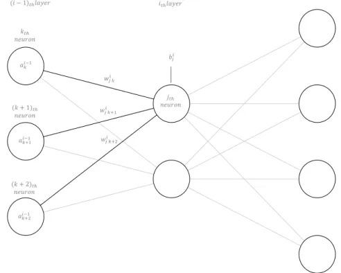
Before defining and exploring in greater detail the propagation, activation and cost functions, it is imperative to define a terminology for the different components of an artificial neural network (ANN) architecture. In ANNs, neurons are distributed in layers – at least two, the input and the output layer. Generally, the neurons from one layer are connected to all the neurons from the antecedent and the preceding layers. Considering only the interactions between the jthneuron in the ithlayer of the network and all its connections from the previous layer, as shown in figure3.1.

The following notation applies:

• wi_jk is the weight of the connection between the jth neuron in the ith layer and the kthneuron from the previous layer;

• bi_j is the weight of the bias term, sometimes also interpreted as bi_j= ωi_j0. The bias term is constant and equal to 1, the same for all the neurons in the network, and its weight only changes in order to allow for shifts in the activation function; • ai−1_k is the output of the k_th neuron in the (i − 1)_th layer of the network. Let

zi_j = f (ωi_jk, ai−1_k ) and σ (zi_j) be respectively the propagation and the activation functions yet to be defined. Then: ai_j = σ (zi_j).

(27)

3 . 2 . C O M P O N E N T S O F A R T I F I C I A L N E U R A L N E T WO R K S 𝑎_𝑘𝑖−1 𝑎𝑘+1𝑖−1 𝑎𝑘+2𝑖−1 𝑖𝑡ℎ𝑙𝑎𝑦𝑒𝑟 𝑗𝑡ℎ 𝑛𝑒𝑢𝑟𝑜𝑛 (𝑖 − 1)𝑡ℎ𝑙𝑎𝑦𝑒𝑟 𝑤𝑗 𝑘𝑖 𝑤𝑗 𝑘+1𝑖 𝑤𝑗 𝑘+2𝑖 𝑏𝑗𝑖 𝑘𝑡ℎ 𝑛𝑒𝑢𝑟𝑜𝑛 (𝑘 + 1)𝑡ℎ 𝑛𝑒𝑢𝑟𝑜𝑛 (𝑘 + 2)𝑡ℎ 𝑛𝑒𝑢𝑟𝑜𝑛

Figure 3.1: Three Layer Neural Network.

3.2.1 Propagation Function

Each neuron i receives multiple input connections, either direct inputs of the problem at hand or outputs of other neurons and aggregates all this stimuli into a single signal using a propagation function:

f = f (wi_jk, ai−1_k )

Although this net signal could be calculated using innumerous functions, the most common propagation function is an inner product between the vector of weights and the vector of neuron outputs:

f (w_jki , ai−1_k ) = zi_j= n X k=0 ωi_jk∗_ai−1 k = n X k=1 ωi_jk∗_bk j 3.2.2 Activation Function

Biological neurons respond differently according to the received stimuli. If the resul-tant signal is above a certain threshold, the neuron sends an electrical signal, or a spike, along its axon. In artificial neural networks, the assumption is that the precise timings of the spikes are not relevant, but it is rather their frequency that holds the information [14]. To model this behavior, a function representing the frequency of the spikes along the axon is used - the activation function.

(28)

Using the previous notation, the activation function σ is such that:

ai_j = σ (zi_j)

Different functions can and have been used as activation functions. The most basic activation function is the binary threshold function or Heaviside function. It is defined as: σ (zi_j) =          0 if z_ji< 0 1 if z_ji≥₀

The function takes only two possible values and is not differentiable at zi

j = 0. As

such, learning algorithms as backpropagation cannot be used.

A historically popular choice for the activation function was the sigmoid function, which is a special case of the logistic function and is defined as:

σ (zi_j) = 1

(1 + e−zij₎

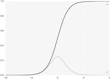
As for the Heaviside function, the sigmoid outputs values between 0 and 1, how-ever unlike the first it is continuous and therefore differentiable. The drawback with this activation function is that it promotes what is known as the vanishing gradient problem if the network uses gradient based methods to learn [20].

Essentially, if a change in a parameter’s value causes very small changes in the network’s output, then that parameter cannot be learnt effectively. This can be easily seen by analyzing the expression for the update of the weights using backpropagation, which is dependent on the first derivative of the activation function (please refer to the next section on Neural Networks Architecture for further details).

For the case in which the activation function σ is the sigmoid function:

σ (zi_j) = 1 (1 + e−zji₎ ⇒_σ0_(zi j) = e−zij (1 + e−zij₎2

For both large and small inputs, the derivative is very close to zero, thus killing the gradient and making the learning process harder. This effect can be observed in figure

3.2. The issue worsens when multiple layers of neurons are used.

Several functions have been found to overcome this issue. In particular, the Rec-tified Linear Unit (ReLU) has become very popular in the last few years. It is defined as:

σ (zi_j) = max(0, zi_j)

This function was found to greatly accelerate the convergence of stochastic gradient descent compared to the sigmoid functions, allegedly due to its linear, non-saturating form [22].

(29)

3 . 2 . C O M P O N E N T S O F A R T I F I C I A L N E U R A L N E T WO R K S

𝜎′

𝜎

Figure 3.2: The sigmoid activation function and its derivative.

The previous examples of activation functions depended only on the net value of the input for a specific neuron j. However, activation functions might also take into consideration the inputs of the other neurons in the same layer. One case of such functions is the softmax function, also known as the normalized exponential. It is defined as: σ (zi_j) = e zi j P kez i k

Although this activation function can be used in any layer of the network, it is usually used in the last. As a consequence of the mathematical definition of this function, the outputs of the network are always positive and sum up to one. This can be easily proven using the properties of summations and the exponential function:

ezij_{> 0 ∀z}i j ∈ R ⇒ ezji P kez i k > 0 ∀zi_j∈ R X j σ (zi_j) =X j ezij P kez i k = P je zi j P kez i k = 1

Being always positive and adding up to one, the outputs of a softmax layer can be thought of as belonging to a probability distribution. In many cases this interpretation might be convenient. For instance, in a classification problem the output of a the softmax layer will be the probability of a chosen input to belong to a certain class. 3.2.3 Cost Function

Learning to perform a task usually requires several trials – each successive trial should be an attempt to improve on the results achieved in the past. Learning systems, and in

(30)

particular neural networks, follow the same approach: in each iteration, the network gives an output that is compared with the true value. This comparison operation is performed by a cost function, and its result is used to modify the weights of the connections in the network, thus allowing the network to better shape the solution surface. In principle, the more different the real and the expected output are, the larger will be the modifications in the network’s weights.

Using the previously defined notation and representing y_ji as the correct output of the jthneuron in the ith layer of the network, the cost function E is such that:

E = E(ai_j, y_ji)

Multiple cost functions may be used, the simplest and most common of all being the quadratic cost, also known as squared error, maximum likelihood or sum squared error. Let n be the number of training examples. Then the quadratic cost is defined as:

E_ji= 1 2n n X x=1 (ai_j−_yi j)2

Although the quadratic cost is a popular choice for the cost function, it has a major disadvantage if the activation function chosen for the network is the sigmoid. Learning is expected to be faster when the difference between the real and the expected output (the error) of the network is larger, however this premise may be compromised if using this cost function, as the update of the connection weights is proportional to the derivative of the activation function [27] (please refer to the next section on Neural Networks Architecture for further details). If this function is the sigmoid, the derivative is very close to zero to either large or small outputs (neuron saturation), as seen before. As such, even if the error is large, the update in the weights will be small:

∂E_ji ∂ωi_jk = (a i j−yji)ω 0 (z_ji)ai−1_j ∂E_ji ∂bi_j = (a i j−yji)ω 0 (zi_j)

In order to overcome this issue, a common solution is to use a cross-entropy cost function, which is defined as:

E = −1 n n X x=1 y_jiln(ai_j) + (1 − y_ji) ln(1 − ai_j)

This cost function was developed precisely to fix the learning slowdown problem presented before. Making use of a property of the sigmoid function, whose deriva-tive can be written as a function of the sigmoid itself, it can be easily seen that the derivatives are no longer dependent on σ0(zi_j):

(31)

3 . 3 . N E U R A L N E T WO R K S A R C H I T E C T U R E S σ (z_ji) = 1 1 + e−zij ⇒_σ0_(zi j) = e−zij (1 + e−zij₎2 = 1 1 + e−zij ×_{(1 −} 1 1 + e−zij ) = σ (zi_j) × (1 − σ (zi_j)) ∂E_ji ∂ωi_jk = 1 n n X x=1 σ0(z_ji)ai−1_j σ (z_ji) × (1 − σ (z_ji))(σ (z i j) − yji) = 1 n n X x=1 (ai_j−_yi j)ai−1j ∂E_ji ∂b_ji = 1 n n X x=1 (ai_j−_yi j)

Therefore, the cross-entropy cost function is the most common choice whenever the activation function is the sigmoid.

3.3 Neural Networks Architectures

Several different network architectures exist, however their basic learning principle is the same: to find the vector of weights [wi_jk] and bias [bi_j] that minimizes the differ-ence between the actual and the expected output of the network. In this section, the two main existing architectures and their most common learning methodologies are analyzed.

3.3.1 Feedforward Neural Network

In feedforward networks, information flows in only one direction, from the input nodes, through (possible multiple or none) hidden layers of neurons and finally to the output nodes. The simplest example of such architecture is a single layer network.

For this simple example, the delta rule, which is based on gradient descent, is applied as the learning mechanism of the network. According to this rule, the weights of the network should be modified in the following way:

wi_jk= wi_jk+ ∆w_jki

∆wi_jk= −η ∂E

∂wi_jk

Here η is an adjustable parameter called learning rate which regulates the magni-tude of the update. As this network has no hidden layers, there are only connections between the input and the output layer. As such, the index i may be ommited from the previous expressions. Furthermore, only the neurons from the output layer are responsible for performing computations and their output is also the final output of the network. As such, the associated error is clearly defined – both the output of the neuron and the expected output are known - and its exact form is only dependent on

(32)

the chosen cost function E. For example, in the case in which the cost function is the quadratic cost: ∂E ∂ωjk =∂E ∂σ ∂σ ∂ωjk = (aj−yj)σ 0 (zj)

As demonstrated before, the derivative of the sigmoid function can be written as a function of the sigmoid itself. For this case, the previous expression may be written as:

σ0(zi_j) = σ (zi_j) × (1 − σ (zi_j)) ∂E ∂ωjk = (aj−yj)σ 0 (zj) = aj(1 − aj)(aj−yj)

A similar methodology is followed for multilayer feedforward networks. The dif-ference between these and the single layer network analyzed before is the existence of hidden layers of neurons between the input and the output layers. This fact trig-gers a crucial observation - only the expected outputs of output layer of the network are known, as they correspond to the targets on the training data used. There is no information on what the outputs of the hidden neurons should be. As such, instead of the delta rule, a more general method should be used, the most common of which is backpropagation. Backpropagation may be decomposed in one forward step and one backward step. In the forward step, the weights of the connections remain unchanged and the outputs of the network are calculated propagating the inputs through all the neurons of the network. The backward step consists in the modification of the weights of each connection:

• For the output neurons, the modification is performed as before, by means of the delta rule;

• For the hidden neurons, the modification is done by propagating forwards the error of the output neurons: the error of each hidden neuron is considered as being equal to the sum of all the errors of the neurons of the subsequent layers.

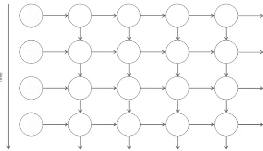
3.3.2 Recurrent Neural Network

In feedforward neural networks, information flows in a single direction - from the input layer directly to the output layer. Recurrent neural networks (RNNs) do not impose such constraints, thus allowing for the existence of loops in the architecture. As such, each neuron in the hidden layer receives not only the inputs from the previous layer in the network, but also its own outputs from the last time step. This structure is shown in figure 3.3. The same architecture can be represented more clearly by unfolding the network along the time axis, as shown in figure3.4.

(33)

3 . 3 . N E U R A L N E T WO R K S A R C H I T E C T U R E S

Figure 3.3: Basic Structure of a Recurrent Neural Network.

Tim

e

Figure 3.4: Unfolded Recurrent Neural Network along the time axis.

In this representation, each horizontal line of layers is the network running at a single time step. Each hidden layer receives both input from the previous layer and input from itself one time step in the past.

The cyclic nature of recurrent neural networks allows them to maintain context on past events, making them best suited for modeling sequential processes, such as time series, text, and music. Although in theory the above architecture should be able to explore long term dependencies in a chain of events, it has been proven that due to the vanishing gradient problem the memory is actually very short-term [5].

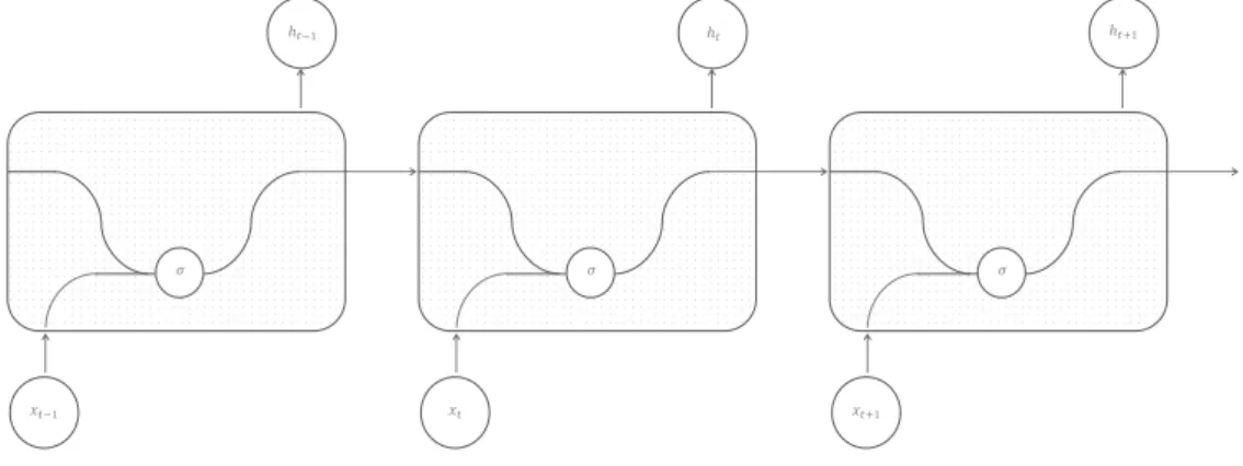
To overcome this issue, the networks neurons can be replaced by a specially de-signed memory cell – a long short-term memory (LSTM) cell, introduced by Hochreiter and Schmidhuber in 1997 [6].

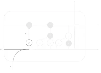
All recurrent neural networks have the form of a chain of repeating modules, but the structure of these models is different between simple RNNs and RNN + LSTM architectures, as can be understood in figures 3.5 and 3.6. In standard RNNs, the repeating module has a very simple structure, with only one activation function to process all the incoming information simultaneously (the output xt of the previous

neurons and its own output h_t−1from the previous time step). In LSTMs, the repeating module has a different structure, as information flows in different paths - part of it is stored in the cell (the state Ct), and another serves as the output (ht), which is

(34)

leaves the cell, with the help of two functions g and σ and a set of bitwise operators [16]. 𝜎 𝑥𝑡−1 ℎ𝑡−1 𝜎 𝑥𝑡 ℎ𝑡 𝜎 𝑥𝑡+1 ℎ𝑡+1

Figure 3.5: Structure of a basic Neural Network cell.

𝑥𝑡−1 ℎ𝑡−1 𝑔 x + x x 𝑔 𝜎 𝑔 𝜎 𝑥𝑡 ℎ𝑡 𝑔 x + x x 𝑔 𝜎 𝑔 𝜎 𝑥𝑡+1 ℎ𝑡+1 𝑔 x + x x 𝑔 𝜎 𝑔 𝜎

Figure 3.6: Structure of a Long-Short Term Memory cell (LSTM).

The advantage of LSTMs over the simple architecture is precisely the ability to control the information that flows through its gates, allowing the implementation of a memory unit - the cell state Ct, which ensures the network can preserve whatever

information from the past that is considered relevant and not lose it after a few time steps. LSTM have three of these gates:

• Forget Gate

Not all the information received is necessarily useful. This layer looks at the output from the previous time-step, ht−1, and the input xt and applies a sigmoid

g to output a number ft between 0 and 1 for each number in the cell state Ct−1,

with 1 represeting “keep” and 0 representing “do not keep the information” (figure3.7):

ft= g(wf ·[ht−1, xt] + bf)

(35)

3 . 3 . N E U R A L N E T WO R K S A R C H I T E C T U R E S x + x x 𝑔 𝜎 𝑔 𝜎 𝑔 𝑓𝑡 𝑥𝑡 ℎ𝑡−1

Figure 3.7: Forget Gate of a LSTM cell.

• Input Gate

The cell state is a unit memory that keeps the information considered relevant. This information can be modified through the input gate. The process is accom-plished in two steps: first a sigmoid g is used to select which values are going to be updated (it) and then an activation function σ (usually a hyperbolic tangent)

is used to generate a vector of candidates C_t0. These two are combined to update the cell state with i_t×_C0

t, where:

it= g(wi·[ht−1, xt] + bi)

C_t0= σ (wC·[ht−1, xt] + bC)

Figure 3.8 represents the operations to calculate it and C

0

t and to update the

current cell state C_twhere, as described before:

Ct= ft×Ct−1+ it×C

0

t

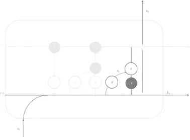
• Output Gate

The information that is considered relevant to keep in the cell’s memory is not necessarily the same that is important to output. This fact motivates the existence of the output gate – its purpose it to select a filtered version of the cell state as output. The process is accomplished in two steps: first an activation function σ (usually an hyperbolic tangent) is applied to the cell state and then its result is multiplied by a sigmoid g applied to the cell input (ot), allowing for only certain

(36)

C H A P T E R 3 . N E U R A L N E T WO R K S ot = g(wo·[ht−1, xt] + bo) ht= ot×σ (Ct) x + x x 𝑔 𝜎 𝑔 ℎ𝑡 𝐶𝑡−1 𝐶𝑡 ℎ𝑡 ℎ𝑡 ℎ𝑡 x 𝑔 𝜎 𝜎 𝑥𝑡 𝑔 𝜎 𝐶𝑡−1 𝐶𝑡 ℎ𝑡−1 x 𝑔 + x 𝑔 𝑓𝑡 _𝑖 𝑡 𝐶′𝑡 𝑥𝑡 ℎ𝑡−1 𝑖𝑡 𝐶′𝑡

Figure 3.8: Input Gate of a LSTM cell.

x + x 𝑔 𝜎 𝑔 𝐶𝑡−1 𝐶𝑡 ℎ𝑡−1 ℎ𝑡 ℎ𝑡 𝜎 x 𝑔 𝑥𝑡 𝑜𝑡

Figure 3.9: Output Gate of a LSTM cell.

An important question may now be answered – why do LSTMs have the ability to avoid the vanishing gradient problem? The LSTM architecture allows disabling of writing to a cell (partially or completely) by controlling the information which goes through the input gate. This prevents too many changes to the cell’s contents over the learning cycles, thus preserving information from early parts of the sequences that are considered relevant. Modeling long term dependencies is, as such, not a difficult task for this network architecture.

(37)

3 . 4 . M E T H O D S T O I M P R O V E L E A R N I N G P E R F O R M A N C E

Recurrent neural networks are trained in a similar way to feedforward neural net-works, however the change in architecture requires an adapted version of the backprop-agation algorithm called backpropbackprop-agation through time [25]. Provided the network is fed with finite time steps [8], it can be unfolded along the time axis, as demonstrated before, and the usual backpropagation algorithm can then be applied.

3.4 Methods to Improve Learning Performance

Learning algorithms are applied to data in which some hidden knowledge is expected to be found. Their goal is to learn this knowledge and code it into the model using a subset of the data for which the targets are known.

The ability to generalize well from this subset is essential to a good model, as it determines its ability to make accurate predictions on unseen data. When models are too specialized on the data they were trained with, they fail to comprehend the inherent process behind it and, as such, predictions tend to be off. This issue is commonly known as overfitting and it can be controlled in a variety of ways, some specific to the model used and some applicable to all the data models.

Focusing on neural networks, the most common techniques for dealing with over-fitting include regularization, dropout and adaptive learning rates:

• Regularization

Different techniques exist, the most popular of which is the L2 regularization, also known as “weight decay”. The concept behind this technique is to add a term to the old cost function E0, such that:

E = E0+ λ 2n X ω ω2

This term is a sum of the squared weights of the network, scaled by a factor _2nλ , where λ is known as the regularization parameter. Its purpose is to control the weights of the network, as larger weights may lead to overfitting. In other words, regularization can be viewed as a way of compromising between finding small weights and minimizing the original cost function. The relative importance of the two elements of the compromise depends on the value of the regularization parameter [27].

• Dropout

Instead of using all the network neurons at each step of the learning process, with dropout part of the hidden neurons of the network are randomly and tem-porarily deleted (or dropped), leaving the input and output neurons untouched.

(38)

The network is then trained over a batch of training examples before a new con-figuration is selected. With this method, the weights and biases are learnt in different conditions, thus preventing overfitting [27].

The concept behind dropout can be compared to the one used in ensemble mod-els [34]– in these, several models vote together to classify the data instances. As they were trained independently, it is expected that these models may have over-fitted the data in different ways and, as such, joining them together may help to overcome their individual weaknesses. The main difference between these techniques is that with dropout the strategy is applied during the training of only one model, instead of after the training with multiple ones.

• Adaptive Learning Rate

Traditionally the learning rate η is the same for all parameters in the model and also constant in time. However, the simplicity in this formulation may have implications in the learning process.

First of all, some parameters may be closer to their optimal value than others at a given time. Therefore, being subject to a common learning rate may not be the best approach to their progress – much like with students in a class.

Secondly, a constant learning rate in time is also not the smartest solution. In the beginning of the training process, a higher learning rate is desirable to speed up the process. However, in later stages of training, lower values for this parameter are preferable because they allow a more thorough search of the solution space in the quest for the optimal solution. Several adaptive learning rate methods have been developed over the years. Particularly interesting are the Adagrad and the RMSprop techniques [30].

With Adagrad, the learning rate is adjusted for each individual parameter. If a parameter has a low gradient, i.e, if it is close to an optimal value, the learning rate will be barely modified. However, if the gradient is high, Adagrad will shrink the learning rate for that parameter. The downside of this method is that the gradient aggressively and monotonically decreases in each iteration and so, there will be a point during training in which the learning rate is so small that effective learning is no longer possible.

RMSPRop aims at resolving Adagrad’s primary limitation, by considering only a portion of the gradients – the n most recent. The learning rate is therefore updated using the formula:

η = √η G, with G = γ × t−1 X t−n (∂E ∂ω) 2_{+ (1 − γ) × (}∂E ∂ω) 2 t 20

(39)

3 . 4 . M E T H O D S T O I M P R O V E L E A R N I N G P E R F O R M A N C E

Here γ is a parameter called the learning rate decay, as it controls the effect of the past gradients on the update of the learning rate.

This formulation prevents the learning rate from decreasing too rapidly and so it allows an effective training.

(40)

(41)

Chapter 4

Data Representation

While data has an intrinsic value and meaning, it can be communicated through differ-ent means and, as a consequence, be understood in different ways. Between humans, the same ideas can be shared with gestures or drawings, be written, spoken and even felt by touch. As such, a critical component of any data modeling task is the choice of the data representation to be used during the processing phase and also, if possible, of the data source itself.

Regarding the sources of data, music has been coded over the years in a variety of ways, with focus on digital audio files, sheet music, abc notation and MIDI files. Each of these possibilities was designed with different end purposes, with their own advantages and disadvantages, which are briefly discussed below.

4.1 Digital Audio Files

When a medium is disturbed, pressure waves are created and propagated from this origin point until they eventually dissipate. A visual example of this phenomenon would be the waves formed on the surface of a liquid when an external object hits its surface. Humans capture these pressure waves through the eardrums, which convert them into a signal that the brain processes as sound. In order to store information on these phenomena, an instrument – usually a microphone – is used to convert the pressure waves into an electric potential with amplitude corresponding to the intensity of the pressure. In this phase, the signal obtained is an analog signal. To convert it to a digital signal used by current audio files, the electrical signal is sampled, by measuring its amplitude at regular intervals, often 44100 times per second. Each measurement is then stored as a number with a fixed precision, often 16 bits.

While digital audio files are rich in the information they contain, the way in which it is stored poses great challenges for data analysis tasks. There is no direct way to know which note is being played at each time and by which instrument. In order to extract information for analysis, processes such as Fourier transforms, beat detection algorithms and frequency spectrograms are usually applied. To extract the necessary

(42)

C H A P T E R 4 . DATA R E P R E S E N TAT I O N

information for a composition or classification task from audio files is therefore not impossible, but rather complex and, as such, it will not be used in this thesis.

4.2 Sheet music and ABC notation

Music has long accompanied the human existence and so has the need to take record of all the pieces composed and played over the millenniums. Since computers are a recent invention in this time frame, visual and symbolic systems for musical representations were used in the past and inherited to the present times. The most common of such systems is sheet music. In this notation, the fundamental latticework is the staff – there are five staff lines and four intervening spaces corresponding to note pitches of the diatonic scale. Different symbols are then displaced in specific positions within those lines to represent the notes played, their duration, the associated rhythm and other musical characteristics.

While highly spread and used, this notation is not simple to learn, in part because it is rich enough to express something as complex as music and in part because it is an old system. More recently, other written forms of musical notation have appeared, as was the case of the ABC notation. In its basic form, this notation uses the letters A through G to represent notes and other elements, always characters or symbols present on a computer keyboard, to add value to the notes – if its sharp or flat, its length, the key or any necessary ornamentation. In a way, ABC notation is a mapping between each character or a group of characters to specific symbols on a sheet music [32].

Because ABC notation is closer to a conventional language system, it is possible to use text mining tools and algorithms to process it. For the specific case of algorithmic composers, it might even be the best option, as it better simulates how humans create music. Furthermore, digital audio files and MIDI files, being continuous, require discretization and a range of possibly restrictive assumptions in order to be used for composition. The downside of using data in the ABC notation for the purpose of music composition is the time and computer resources needed to obtain a satisfactory model, as language modeling is still not an easy task [28].

4.3 MIDI Files

MIDI (Musical Instrument Digital Interface) is a standardized data protocol to ex-change musical control data between digital instruments. It is not a digital audio file and does not even contain any sounds, but rather a set of instructions that tell an elec-tronic device how to generate a certain sound. These instructions are coded into MIDI messages [19], for instance:

• Note On: signals the beginning of a note, how hard it was pressed and at which velocity;

(43)

4 . 3 . M I D I F I L E S

• Note Off: signals the end of the note;

• Control Change: indicates that a controller, such as a foot pedal or a fader knob, has been pressed;

• Pitch Wheel Change: signals that the pitch of a note has been bent with the keyboard’s pitch wheel.

While this format might not be as rich as the previously mentioned notations, it is certainly easier to extract information from it, especially for the purpose of music composition. The information about the notes being played during the music, when they start and end is all completely determined by a sequence of messages that can be easily extracted using any programming language with a MIDI package. As such, this source format will be the one used in this thesis.

In addition to the choice of a data source format, it is imperative to determine the representation of data to be used in the modeling phase itself. In other words, it should be determined what will be the structure of the data the model will receive and aim to predict. For this purpose, a piano roll representation has been chosen, for it is both easy to process by a neural network and simple to construct from MIDI files. A piano roll shows on the vertical axis the notes as on a piano keyboard and displays time on the horizontal axis. When a note is played, it is represented in the piano roll as a horizontal bar vertically positioned according to its pitch and with a width correspondent to its the duration. This continuous representation can be easily discretized into a two-dimensional matrix, with pitch as the first dimension and time as the second dimension. Each element of the matrix will correspond to a chosen time step and will be either a 1, if the note was played during that time step or 0 if it was not [26]. This will be the representation used to construct the composition and classification models in this thesis.

(44)

(45)

Chapter 5

Methodology

The goal of this thesis is to construct a novel music classification algorithm, capable of discriminating between different types of music without explicitly analyzing its characteristics nor the target category to which they belong. This chapter explains the design process behind the construction of the algorithm and the details of its implementation, such as the data preparation and the technical steps required to put the algorithm to work.

5.1 High Level Design and Concept

Classification tasks are usually achieved by exploring a set of extracted features or characteristics of the subjects of study. An algorithm is then responsible for finding patterns that relate those characteristics to the known targets, learning the inherent knowledge hidden in the data.

While some subjects of study might be easy to describe – a description of a person’s face can easily provide an accurate identification - others reveal unexpected di fficul-ties. Music, for instance, is something present in the everyday life, however when asked to describe a song one would always try to reproduce it instead of describing it. Expressing something as complex as music in words is as difficult as it is simplistic and restrictive. And yet, current music classification systems work on the base of melodic and rhythmic characteristics [23]. This fact motivates an important question – would it be possible to design a classification system more similar to the way humans interpret music? This is precisely the goal of this thesis.

To achieve such an ambitious objective, it is first important to understand or at least grasp some ideas on how humans themselves classify songs, so that this behavior can be reproduced artificially. One could say that, with the information of a song’s author or genre, humans know what to expect of a song. Even more, knowing that same genre or author well, humans have the ability to improvise a more or less reliable excerpt of that musical type. These observations are as obvious as they are revealing, for they suggest the knowledge of these different musical types is intrinsically connected with

(46)

C H A P T E R 5 . M E T H O D O L O G Y

the ability to compose them.

Artificial composition systems have already been explored over the years. It is relatively clear that, providing different types of music to such systems, they should learn to compose different types of songs. If this assumption holds true, and given the conclusions stated before, then these systems possess the necessary knowledge to classify songs.

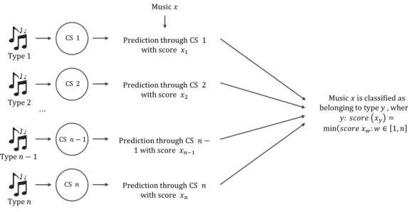
The following statements summarize the concept of the classification algorithm proposed in this thesis:

• Given n artificial composition systems, if each is trained using data from a spe-cific type of music, then each should be specialized in this type only.

• If there exists a substantial difference between these musical types, then it is expected that a system specialized in type 1 will be more successful composing songs belonging to this type than any of the remaining n − 1 systems.

• If a song belonging to one of the n types of music is provided to each of the n composition systems, each will try to compose it and achieve different degrees of success, measurable using a comparison between the predicted song and the real one. A classification algorithm can then be based on this measure – the type of music in which the most successful composition system is specialized will be the one attributed to the song.

CS 𝑛 … CS 𝑛 − 1 CS 2 CS 1 Type 1 Type 2 Type 𝑛 − 1 Type 𝑛 Music 𝑥 Prediction through CS 1 with score 𝑥1 Prediction through CS 2 with score 𝑥2 Prediction through CS 𝑛 − 1 with score 𝑥𝑛−1 Prediction through CS 𝑛 with score 𝑥𝑛 Music 𝑥 is classified as belonging to type 𝑦 , where:

𝑦: 𝑠𝑐𝑜𝑟𝑒 𝑥𝑦 =

min 𝑠𝑐𝑜𝑟𝑒 𝑥𝑤: 𝑤 ∈ 1, 𝑛

Figure 5.1: Proposed Architecture of the Classification System.

The model described before is the basic classification model to be tested and imple-mented in this thesis. A more robust solution will be also impleimple-mented, by substituting each of the n composition systems, consisting of a single RNN + LSTM architecture,

(47)

5 . 2 . DATA P R E PA R AT I O N

by a tree of such structures. With this tweak, a voting system can be implemented – several systems are trained with the same type of music and, given a new song, the average of its prediction score in the various systems is taken, instead of the score of a single system. This will possibly correct some existing overfitting and make the model more stable and robust. As a disadvantage, the training is also expected to be more time consuming and, as such, the possible benefits of this option will be explored ahead.

5.2 Data Preparation

Every data exploration and modeling task should require an initial step of data prepa-ration. Data preparation can be defined as the process of collecting, cleaning, and consolidating data in a structured way, making it ready for analysis.

Particularly important in this thesis is the transformation of the data from the MIDI format to a piano-roll or matrix representation. Data quality procedures will also be taken to ensure that the song matrices are a reliable representation of the music that originated it.

5.2.1 Details on the Matrix Representation

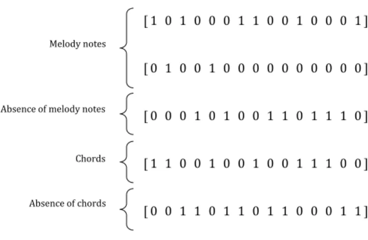
Music can be understood as an interplay of melody and harmony. The first is defined as a linear succession of musical notes, while the second refers to the use of simultaneous notes, i.e., chords. In this thesis, this dual interpretation of music is adopted. Each music can then be represented in a piano-roll or matrix format. Let rmbe the number

of melody notes and r_c the number of chords played. If the song is divided into t temporal steps, then it can be represented as a matrix of size (rm+ rc+ 2) × t where each

element is either one, if the note/chord was played in that time step, or zero if it was not [31]. The plus 2 term exists to account for the cases in which no chord or melody note is played.

Given this representation, what does the algorithm aim to learn? A composer has the knowledge to play the next note based on the past context, such as a writer knows what the next word in a sentence should be to give it meaning. Learning how to write or compose is to develop the ability to know what comes next or, in algorithmic terms, to learn to predict at each step t the vector describing the notes and chords played at

t + 1.

This formulation would imply that the learning targets would be vectors of size (rm+ rc+ 2), where each element of the vector could be either one or zero. However,

there is one issue with such formulation – its complexity.

There are two possible states for each note or chord considered at each time step, which means there are 2(rm+rc+2)_{possible configurations for the target vector, making}

(48)

C H A P T E R 5 . M E T H O D O L O G Y [ 1 0 1 0 0 0 1 1 0 0 1 0 0 0 1 ] [ 0 1 0 0 1 0 0 0 0 0 0 0 0 0 0 ] [ 0 0 0 1 0 1 0 0 1 1 0 1 1 1 0 ] [ 1 1 0 0 1 0 0 1 0 0 1 1 1 0 0 ] [ 0 0 1 1 0 1 1 0 1 1 0 0 0 1 1 ] Melody notes

Absence of melody notes

Chords

Absence of chords

Figure 5.2: Sample Matrix with 15 time steps, 2 melody notes and 1 chord.

a constraint is added to the previous formulation: in each time step, a maximum of one melody note and one chord are allowed. With this rule, the number of possible configurations becomes (rm+ 1) × (rc+ 1).

Considering a practical example, a lower estimate of the number of melody notes and chords in a dataset would be rm≈40 and rc≈10, respectively. This setting would

give 2(40+10+2)≈_{4.5 × 10}15_{possible states per each time step for the naïve formulation} against (40 + 1) × (10 + 1) ≈ 4.5 × 102for the more restrictive formulation – a difference of 13 orders of magnitude. Naturally, the first formulation is richer and a closer rep-resentation of the original music, but given the computational power of the machines used in this thesis, the second formulation is clearly more appropriate.

5.2.2 Dataset

Before explaining the technical steps needed to construct the binary matrix repre-sentation, it is important to understand what data is going to be used and how it is structured.

In theory, any collection of MIDI files may be translated into the previously de-scribed representation. However, the data preparation involved could be expensive, as MIDI files may contain information from various instruments. Usually, each instru-ment is coded in a specific channel and there is no indication what instruinstru-ments are responsible for the melody and which are assigned to the harmony.

To overcome this situation, and as the data preparation is not the primary goal of this thesis, the Nottingham dataset was chosen, as the majority of its songs have already been coded in only two channels: one dedicated to the melody notes and the other dedicated to the chords. This dataset is a collection of 1037 British and American folk tunes, containing different categories of songs (jigs, christmas songs, etc.).

(49)

5 . 2 . DATA P R E PA R AT I O N

Each song in the dataset is subject to a set of procedures, which are performed automatically through a script. The Python language was chosen not only for this section, but for this thesis as a whole, for it is intuitive and simple, but mainly because it is an open source language with excellent packages in data science and also music.

5.2.3 MIDI file to matrix representation

Once the dataset has been chosen, the MIDI files can be analyzed one by one in order to construct a suitable matrix representation. However, it is imperative to fully under-stand the information contained in such files so that the process can be as accurate as possible, ensuring minimum loss or disruption of information.

MIDI files are organized in tracks, which are a collection of messages containing relevant data. Each track is normally assigned to a specific instrument, but this is not mandatory. In the case of the Nottingham dataset, the majority of songs have 3 tracks – one track for the metadata, another for the melody and the final one dedicated to the harmony, which is precisely the structure needed to construct the matrix representa-tion presented before. As such, all the songs that do not respect this structure have not been considered.

Each MIDI track is a collection of messages, the most important of each are the NoteOn, NoteOff and EndOfTrack, which designate the beginning of a note, the end of a note and the end of a track, respectively. Below is an example of a sequence of such messages, extracted with the help of the Python “MIDI” package, which provides functions to open the files and easily extract information from the tracks:

midi.NoteOnEvent(tick=1, channel=0, data=[78, 105]) midi.NoteOffEvent(tick=479, channel=0, data=[78, 0]) midi.NoteOnEvent(tick=1, channel=0, data=[76, 80]) midi.NoteOffEvent(tick=239, channel=0, data=[76, 0]) midi.EndOfTrackEvent(tick=26, data=[])

As observed in the example above, each message contains a set of information. Starting from the end of the message, the array “data” contains two elements, the first of which is the pitch of the note being played (in MIDI numbers) and the second being the velocity with which the note has been played (in case of the piano, it would correspond to how hard a key was pressed). The next element attributes a “channel” to the message (a different instrument, for example). Finally, the first element of the message is the “tick” value. Ticks represent the lowest level of resolution of a MIDI track, which is precisely defined has:

Resolution = N umber of T icks