SequenƟ al Sampling of Aphis gossypii Glover (Hemiptera: Aphididae) and

journal homepage: www.scielo.br/ne

ISSN: 1519-566X

PEST MANAGEMENT

Sequen

Ɵ

al Sampling of

Aphis gossypii

Glover (Hemiptera: Aphididae) and

Frankliniella schultzei

Trybom (Thysanoptera: Thripidae) on Co

Ʃ

on Crop

MG F

›Ùăė›Ý

1

_{, RR S}

֛ÝÝÊãÊ

2

_{, PE D}

›¦ÙƒÄ—›

3

_{, TR R}

ʗٮ¦ç›Ý

4

1_{Programa de Pós-Graduação em Entomologia e Conservação da Biodiversidade,} 2_{Fac de Ciências Biológicas e Ambientais,} 3_{Fac de Ciências}

Agrárias, 4_{Fac de Ciências Biológicas e Ambientais. Univ Federal da Grande Dourados, Dourados, MS, Brasil}

Keywords

Control level, coƩ on aphid, IPM, thrips

Correspondence

MƒÙ‘ÊÝ G F›Ùăė›Ý, Faculdade de Ciências Biológicas e Ambientais, Univ Federal da Grande Dourados, Rod Dourados-Itahum, km 12, Cidade Universitária, CP 533, 70804-970, Dourados, MS, Brasil; marcosfernandes@ ufgd.edu.br

Edited by Wesley A C Godoy – ESALQ/USP

Received 04 December 2009 and accepted 11 August 2010

Abstract

The goal of this research was to use the sequential probability ratio test to establish a sequential sampling plan for Aphis gossypii

Glover and Frankliniella schultzei Trybom infesting cotton. Field

work was conducted at the agricultural experimental station of the Universidade Federal da Grande Dourados during the 2003/2004 and 2004/2005 agricultural years. Aphid colonies and individual thrips in the sampling area were counted and their numbers were recorded. The spatial distribution pattern of A. gossypii and F. schultzei in the

cotton culture was aggregated. Sequential sampling plans were developed for aphids and thrips with type I and type II errors set at 0.1, common Kc = 0.6081 (aphids) and = 0. 9449 (thrips), and safety and management levels of 20% (aphids) and 40% (thrips) of infested plants. The sampling plans resulted in two decision boundaries for each species, as follows: the upper boundary, indicating when management (population control) is recommended: S1 = 4.6546 + 0.2849n (aphids), and S1 = 3.6514 + 0.1435n (thrips); and the lower boundary, indicating when population control is not necessary: S0 = -4.6546 + 0.2849n (aphids) and S0 = - 3.6514 + 0.1435n (thrips). The highest probability of error when making a decision was 3% for aphids and 2% for thrips, respectively. The maximum number of samples required to reach a decision was 63 for aphids and 95 for thrips.

Introducti on

Decision making is a key aspect of current integrated pest management (IPM). In an IPM context, decision making relies on protocols for deciding on the need for some management action based on an assessment of the pest population level (and its natural enemies whenever possible). Consequently, sampling plans are a crucial component of IPM decision guides, because they allow for an estimate of pest counts, and pest counts is an important factor to consider when deciding whether or not to control.

In spite of the technological advances that the last decade has brought to the management of cotton cultures in South America, some insects such as the aphid Aphis gossypii Glover and the thrips Frankliniella schultzei

Trybom have become key pests in several producing regions (Barros et al 2006, Sujii et al 2007). When trying

to devise sampling plans that will work for these pests, it is necessary to know some of their biological peculiarities and their behavior in the ield (Gencsoylu & Yalcn 2004), and to incorporate ecological principles in the sampling process (Fernandes et al 2006).

Wald (1947) and has been widely used in entomology since the 1950s, but particularly after the 1970s. Broad studies conducted in large areas usually deal with the distribution of insect species and are used to predict damage and/or to access the need for control measures. The same area can be sampled several times during a given period of time, focusing on the same life stage of the insect (in which case the sampling period needs to match the life-stage chosen) (Kuno 1991). These studies usually provide information on the population dynamics at a given area along the years, making it possible to correlate population levels with certain edaphic and climatic factors

(Kaplan & Eubanks 2002).

Sequential sampling has been shown to be faster and more reliable than conventional sampling. In contrast to the latter technique, in which a ixed number of samples are used, sequential sampling can minimize survey effort because the number of samples required depends on the size of the population under survey (Kogan & Herzog 1980). Intensive studies include continuous observations of a local population over a period of time. Usually, the information gathered by these studies allow for the construction of life tables, assessment of parasitism levels, dispersion rates, and changes in the population; they also help to determine factors that cause and regulate large luctuations in population size (Qaim & Zilberman 2003).

Ruesink & Kogan (1975) proposed the probability ratio method to develop sequential sampling protocols for insects. In order for this method to work, the following requirements need to be met: 1) a probability function that describes the spatial pattern of the insect needs to be found; 2) the economic injury levels need to be established as two critical densities, such as: economic injury will take place when the insect density surpasses an upper boundary, and will not take place when the insect density stays below a lower boundary; 3) the highest probability levels of making mistakes in estimating insect densities need to be selected [i.e. the probability of predicting an insect density as non-harmful when it is so (a type I error), and the probability of predicting an insect density as harmful when it is not so (a type II error)].

Regarding to the irst requirement, Fernandes et al

(2003) classi ied the spatial pattern of organisms in the ield into aggregated, uniform, or random. These can be statistically described as negative binomial, positive binomial and Poisson, respectively. Each spatial pattern involves a different set of parameters, requiring the use of different methods to establish a sampling plan. The second requirement has rarely been studied in Brazil, as it involves long-term studies that cover successive crop cycles, as for instance knowledge about the physiology of the crop and estimates such as pest damage, control costs and crop value. The rarity of such studies has hindered the design of sequential sampling plans in the country

(Barbosa 1992).

Sequential sampling can be applied to agroecosystems as well as natural ecosystems. In entomology, sequential sampling is often used to accomplish the following tasks: to determine different properties of a population (such as density, birth rate, mortality rate, age distribution, the biotic potential, dispersal, growth pattern and ecological-related genetic traits); to determine when pest control is necessary (action level); to access ecological interactions between species; to access the degree of plant resistance to herbivores, and the effects of management on non-target species. Moreover, it is possible to use the sequential sampling method for the quick and precise determination of the right time to start an experiment, to evaluate the population of a target pest, or to test the ef iciency of an insecticide or the release of natural enemies as part of biological control studies (Fernandes

et al 2003).

Therefore, the goal of this research was to establish sequential sampling plans for A. gossypii and F. schultzei,

two important pests of cotton, following Wald’s sequential probability ratio test (SPRT).

Material and Methods

DescripƟ on of the experimental area

Field work was conducted at the agricultural experimental station of the Universidade Federal da Grande Dourados (UFGD), district of Dourados (22º14’S, 54º44’W, 452 m), Mato Grosso do Sul, on a distroferric red latossoil (Mato Grosso do Sul 1990). The plant cultivars Fibermax 986®

and DeltaOpal® _{were used during the 2003/2004 and}

2004/2005 agricultural years, respectively. The plot was divided into 100 sampling squares of 100 m² (10 m x 10

m) each. Six plants were randomly inspected along the central line of each sampling square (except for plants on the borderlines), totaling 600 plants per sampling effort. During inspection, the entire plant was examined.

Samplings

The total number of aphid colonies (A. gossypii) and

the total number of individual thrips (F. schultzei) were

recorded. We considered a “colony” any assemblage with at least 20 individuals, including nymphs and adults. Sampling was conducted every three days from December 2003 to February 2004, then from December 2004 to February 2005. Throughout the duration of this study, no insecticides targeting either A. gossypii or F. schultzei or

any other insects were used in the sampling area.

Establishment of sampling plans

mathematical description of the spatial dispersion of each population. In both cases, ield data conformed to the expected distribution of the negative binomial model. The sampling plans developed for each species are based on the SPRT, following the method developed by Wald (1947) and adapted by Young & Young (1998). The goal was to test the hypotheses H₀ and H₁ based on the fewest possible number of samples. The null hypothesis (H₀ ) predicts that the population number is below the safe threshold, and accepting it results in no need to control the population; the alternate hypothesis(H₁)predicts that the population number is above a safe threshold and accepting it results in the need to take population control measures (Fernandes et al 2003).

The decision boundaries necessary to conduct the SPRT were constructed. The upper decision boundary indicates the population density above which control is necessary. The lower decision boundary indicates that population densities are within or below a secure threshold and therefore there is no need for control.

The decision boundaries of the test are de ined as follows: S₁= h₁+ Sxn (upper boundary) and S₀ = h₀ + Sxn (lower boundary). In these equations, n is the appropriate sample number and values for h_0, h₁ and S are de ined as a function of the negative binomial as:

(

)

(

)

⎥_⎦ ⎤ ⎢ ⎣ ⎡ + + = k k In a h 1 0 0 1 1 μ μ μ μ

(

)

(

)

⎥_⎦ ⎤ ⎢ ⎣ ⎡ + + ⎥ ⎦ ⎤ ⎢ ⎣ ⎡ + + = k k In k k In k S 1 0 0 1 0 1 μ μ μ μ μ μ where: ⎟ ⎠ ⎞ ⎜ ⎝ ⎛ − = α β 1 In a ; ⎟ ⎠ ⎞ ⎜ ⎝ ⎛ − = α β 1 In b

; μ0 = safe threshold; μ1 = economic injury threshold; α= type I error; β= type II

error; k = Kc index (common k) calculated by the method proposed by Bliss & Owen (1958), or:

∑

∑

= i i i i i i x w y x w Kc i 2 , , , 1 where: i i i i n s X x 2 2 , −

= ; yi =si −Xi

2 ,

; n_i = sample

size;

2

i

s _{= sample variance;}

i

X _{= estimated mean; and}

(

)

⎟ ⎟ ⎟ ⎟ ⎠ ⎞ ⎜ ⎜ ⎜ ⎜ ⎝ ⎛ − ⎟ ⎠ ⎞ ⎜ ⎝ ⎛ ₋ − ⎟ ⎠ ⎞ ⎜ ⎝ ⎛ + ⎟ ⎠ ⎞ ⎜ ⎝ ⎛ + − = 2 ^ ^ ^ 2 ^ 2 ^ 4 1 3 1 2 1 1 5 . 0 i i c c c c i i c i n n k k k k X X k n w

As the variable w1 includes the unknown parameter Kc, the process of estimating this variable is iterative and the initial estimate of kc is obtained as following:

∑

∑

=

i i c

x

y

x

k

2 . , , ^

1

In order to determine the decision boundaries, n equals 1 in the irst observation and the upper and lower boundaries are calculated for sample number 1. In the second observation, n equals 2 and the upper and lower boundaries are calculated for sample number 2 and so forth, until the last sample necessary to complete the sampling plan.

The validation of Wald’s SPRT is based on the curve of operating characteristics CO(p) and the curve of expected sample number E_p(n). Therefore, after establishing the sequential sampling plan, it is important to calculate the CO(p), the graphic representation of the operating characteristic function. This curve gives the probability of stopping the sampling and deciding not to control the population as a function of a given insect density. The E_p (n), on the other hand, indicates the mean sample number necessary for decision-making. The equations used to determine both curves are given by Young & Young (1998) as follows:

( )

(

)

(

) ( )

α β α βα β − − − − − = 1 1 1 1 h h p CO

Ep

( )

n CO

( )(

p _ph _Sh

)

h

−

+

−

= 0 1 1

Where p = average number of colonies (aphids) or individuals (thrips) per plant; h = auxiliary variable dependent on p.

Results and Discussion

Aphis gossypii

level (μ₁) was 0.4 (40% of plants infested by colonies), following the recommendations of Degrande (2004). The safe threshold (μ₀) adopted was 0.2 (20% of plants infested by colonies). The parameter K (Kc) was 0.6081. The values adopted for type I and type II errors were  ₌  _{= 0.10. These values were considered appropriate for}

entomological studies by Young & Young (1998). Given the values above, the upper boundary to accept H₁: μ₁ = 0.4 is: S₁ = 4.6546 + 0.2849n; and the lower boundary to accept H₀: μ₀ = 0.2 is: S₀ = - 4.6546 + 0.2849n.

Considering the values resulting from the upper and lower decision boundaries of the sampling plan, a sequential plan was proposed to be used in the integrated management of the aphids. A graph was constructed (Fig 1) based on the numbers resulting from the equations drawing the upper and lower boundaries. S₀ and S₁ were calculated for each value of n. Based on this graph, a table to facilitate the sequential sampling in the ield can be constructed in the following manner: when the irst observation was made (sample # 1), the number of colonies found was recorded in the equivalent “total sampled” ield. The number of colonies found in the second observation was then added to the number found in the irst observation, and the resulting amount was recorded in the “total sampled ield” as “sample #” 2. This process was repeated iteratively until the rule to inalize the sampling was satis ied. The rule to inalize the sampling can be satis ied when either one of the following conditions is met:

1) The total number of colonies counted equals or exceeds the upper boundary. In this case, control is recommended.

2) The total number of colonies counted is less than or equal to the lower boundary. In this case, management is not recommended.

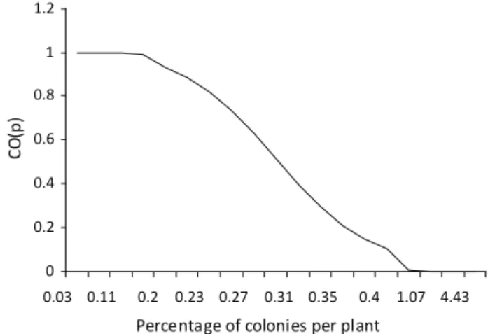
The CO(p) (Fig 2) is a graphic representation of the operating characteristic function that gives the probability that sampling will be stopped and management will not be advised when management is in fact necessary,

or else, that management will be deemed necessary when it is not. Thus, when the mean population density of A. gossypii corresponds to 20% of plants infested

with colonies (at least one, or more), the test has a 1% probability of recommending management when it is unnecessary (type I error). When the mean population density corresponds to 40% of plants infested, the test has only a 0.09% probability of accepting H₀ and not recommending intervention when it is in fact necessary. Above this threshold, the probability of incurring type I error and not recommending intervention when it is necessary nears 0%.

The Ep(n) is a graphic representation of the mean number of observations necessary to reach a decision to control or not, and is dependent upon p. The results for the expected number of samples Ep(n) obtained from Wald’s SPRT (Fig 3) indicates that, when 0.15% or 15% of the plants are infested with colonies, a maximum of approximately 17 samples are needed. When 0.31% or 31% of the plants are infested, approximately 63 samples are necessary to reach a decision.

Fig 1 Sampling plan for the number of colonies of Aphis gossypii,

based on the negative binomial distribution (NAC = Number of accumulated colonies).

Fig 2 Curve of operating characteristics CO(p) for the sampling of Aphis gossypii, based on the sequential probability ratio test (SPRT).

Fig 3 Curve of expected (average) sample number Ep (n) for the

sampling of Aphis gossypii based on the sequential probability ratio

test (SPRT) for the total population.

0

5

10

15

20

25

30

35

40

1 10 19 28 37 46 55 64 73 82 91 100 Number of sampling un its

Accept H1 : μ1 = 0,4

S1= 4.6546 + 0.2849 n

Accept H0 : μ0 = 0.2

S0= - 4.6546 + 0.2849 n

Con nue sampling

NAC

0 0.2 0.4 0.6 0.8 1 1.2

0.03 0.11 0.2 0.23 0.27 0.31 0.35 0.4 1.07 4.43 Percentage of colonies per plant

CO

(p)

0 10 20 30 40 50 60 70

0.03 0.11 0.2 0.23 0.27 0.31 0.35 0.4 1.07 4.43 Percentage of colonies per plant

CO

F. schultzei

A density of 20% of plants with symptoms of infestation by thrips was established as the critical density of the economic injury level (μ₁). A density of 10% of symptomatic plants was adopted as the safe threshold (μ₀). The parameter K (Kc) was 0.9449. The values adopted for type I error and type II errors were  ₌  _{= 0.10. Given the values above,}

the upper boundary to accept H₁ : μ₁ = 0.2 was : S₁ = 3,6514 + 0.1435 n. and the lower boundary to accept H₀: μ₀ = 0.1 was: S₀ = -3.6514 + 0.1435 n.

Using the values resulting from the upper and lower decision boundaries, a sequential plan was prepared to be used in the integrated management of the pest concerned. A graph was constructed (Fig 4) based on the numbers resulting from the equations of the upper and lower boundaries. S₀ and S₁ were calculated for each value of n. Based on this graph, a table can be constructed to facilitate the sequential sampling in the ield. The sampling process followed the same description given for A. gossypii (see

previous comments).

The CO(p) (Fig 5) shows that, when 10% of the plants

show symptoms of being infested by thrips, the test has a 1% chance of recommending management when it is unnecessary (type I error). When an average of 20% of the plants is infested, the test has only a 0.12 % probability of accepting H0 and not recommends intervention. Above this level, the probability of incurring type I error and not recommending intervention when it is necessary nears 0%.

The results obtained for the Ep(n) from Wald’s SPRT (Fig 6) indicates that, when 0.1% or 10% of the plants show symptoms of thrips infestation, an approximately maximum number of 61 samples are necessary. When 16% of the plants show symptoms of infestation, 95 samples are necessary to reach a decision.

As the spatial distribution of both A. gossypii and F. schultzei in the cotton culture can be classi ied as

aggregated, it is possible to use the sequential sampling plans we have developed to sample nymphs and adults of both insects.

Our study has shown the ef icacy of the sequential sampling in entomological research, mainly in studies that emphasize the classi ication of insect populations rather than estimation of population parameters. When compared with traditional sampling, sequential sampling results in economy of time and effort. Besides being notoriously ef icient in agricultural settings, it has proved ef icient in different types of environment, making its utilization possible in different areas of entomology.

References

Barbosa JC (1992) A amostragem seqüencial, p.205-211. In Fernandes O A, Correia AC B, Bortoli SA de (eds) Manejo integrado de pragas e nematóides. Jaboticabal, FUNEP, 253p.

Barros R, Degrande PE, Ribeiro JF, Rodrigues ALL, Fernandes MG (2006) Flutuação populacional de insetos predadores associados a pragas do algodoeiro. Arq Inst Biol 73: 57-64.

Fig 5 Curve of operating characteristics CO(p) for the sampling of Frankliniella shultzei, based on the sequential probability ratio test (SPRT).

Fig 6 Curve of expected (average) sample number E_p (n) for the

sampling of Frankliniella shultzei based on the sequential probability

ratio test (SPRT) for the total population.

Fig 4 Decision boundaries of the sequential sampling plan for the

number of colonies of Frankliniella shultzei, based on the negative

binomial distribution.

0 2 4 6 8 10 12 14 16 18 20

1 10 19 28 37 46 55 64 73 82 91 100 Number of sampling units

Accept H₁ : μ1 = 2

S1 = 3.6514 + 0.1435 n

Accept H₀ : μ0 = 2 S0 = - 3.6514 + 0.1435 n

Con nue sampling

PIT

0 0.2 0.4 0.6 0.8 1 1.2

0.02 0.06 0.1 0.12 0.14 0.16 0.18 0.2 0.96 Percentage of plants with thrips

CO(p)

0 10 20 30 40 50 60 70 80 90 100

0.02 0.06 0.1 0.12 0.14 0.16 0.18 0.2 0.96 Percentage of plants with thrips symptoms

Ep(

n

Bliss CI, Owen ARG (1958) Negative binomial distribution with a common K. Biometrika 45: 37-58.

Degrande PE (2004) Níveis de controle das pragas do algodoeiro. Atualidades Agrícolas 1:22-23.

Fernandes MG, Busoli AC, Barbosa JC (2003) Amostragem seqüencial de Alabama argillacea (Hübens) (Lepidoptera: Noctuidae) em

algodoeiro. Neotrop Entomol 32: 117-122.

Fernandes MG, Silva AM, Degrande PE, Cubas AC (2006)

Distribuição vertical de lagartas de Alabama argillacea (Hübner)

(Lepidoptera: Noctuidae) em plantas de algodão. Man Integr Plagas Agroecol 78: 28-35.

Gencsoylu I, Yalcn I (2004) Advantages of different tillage systems

and their effects on the economically important pests, Thrips

tabaci Lind. and Aphis gossypii Glov. in cotton ields. J Agron

Crop Sci 190: 381-388.

Kaplan I, Eubanks MD (2002) Disruption of cotton aphid (Homoptera: Aphididae) – natural enemy dynamics by red imported ire ants (Hymenoptera: Formicidae). Environ Entomol 31: 1175-1183.

Kogan M, Herzog DC (1980) Sampling methods in soybean entomology. New York, Springer-Verlag, 587p.

Kuno E (1981) Sampling and analysis of insect populations. Annu Rev Entomol 36: 285-304.

Mato Grosso do Sul (1990) Atlas multireferencial [S.l.]. Campo Grande, Secretaria de Planejamento e Coordenação Geral, 28p. Qaim M, Zilberman D (2003) Yield effects of genetically modi ied

crops in developing countries. Science 299: 900-902.

Ruesink WG, Kogan M (1975) The quantitative basis of pest management and measuring, p.309-351. In Metcalf RL, Luckmann WH (eds) Introduction to insect pest management. New York, John Wiley & Sons Inc, 548p.

Sujii ER, Beserra VA, Ribeiro PH, da Silva-Santos PV, Pires CSS, Schimidt FGV, Fontes EMG, Laumann RA (2007) Comunidade de inimigos naturais e controle biológico natural do pulgão,

Aphis gossypii Glover (Hemiptera: Aphididae) e do curuquerê, Alabama argillacea Hubner (Lepidoptera: Nocutidae) na cultura

do algodoeiro no Distrito Federal. Arq Inst Biol 74: 329-336. Wald A (1947) Sequential analysis. New York, John Wiley & Sons,

212p.