Online Identification of a Two-Mass System in
Frequency Domain using a Kalman Filter
Niko Nevaranta1 Stijn Derammelaere2 Jukka Parkkinen1 Bram Vervisch2 Tuomo Lindh1 Markku Niemel¨a1 Olli Pyrh¨onen1
1
Department of Electrical Engineering, Lappeenranta University of Technology, FI-53851 Lappeenranta, Finland. E-mail: {Niko.Nevaranta,Jukka.Parkkinen,Tuomo.Lindh,Markku.Niemela,Olli.Pyrhonen,Juha.Pyrhonen}@lut.fi
2
Department of Electrical Energy Systems and Automation, Ghent University Campus Kortrijk, BE-8510 Kortrijk, Belgium. E-mail: {Stijn.Derammelaere, Bram.Vervisch}@ugent.be
Abstract
Some of the most widely recognized online parameter estimation techniques used in different servomech-anism are the extended Kalman filter (EKF) and recursive least squares (RLS) methods. Without loss of generality, these methods are based on a prior knowledge of the model structure of the system to be identified, and thus, they can be regarded as parametric identification methods. This paper proposes an on-line non-parametric frequency response identification routine that is based on a fixed-coefficient Kalman filter, which is configured to perform like a Fourier transform. The approach exploits the knowl-edge of the excitation signal by updating the Kalman filter gains with the known time-varying frequency of chirp signal. The experimental results demonstrate the effectiveness of the proposed online identification method to estimate a non-parametric model of the closed loop controlled servomechanism in a selected band of frequencies.
Keywords: Kalman filter, Non-parametric estimation, Online identification, Short-time DFT, Two-mass
system
1 Introduction
System identification techniques for the diagnostics and condition monitoring of a mechanical system are key tools to enhance the reliability of electrical drives. An adequate system identification technique is of great importance in the process of acquiring a mathemati-cal model that sufficiently represents the essential sys-tem dynamics. In terms of how the collected in-put outin-put data are transformed into a mathemati-cal model, the methods proposed for identification of mechanical systems can be broadly speaking divided into two main categories: parametric identification (Ljung, 2010) and non-parametric identification tech-niques (Heath,2001). Moreover, the identification can be performed in offline or in online mode by time- or frequency-domain observations.
Different time-domain methods based on a least squares criterion are commonly used in off-line identifi-cation of mechanical systems in open-loop (Nevaranta et al., 2014) or closed-loop control (Saarakkala and Hinkkanen, 2015). Similarly, for online identification purposes, some of these methods have been success-fully applied to online parameter estimation by con-sidering their recursive form (Nevaranta et al.,2015a). One of the most widely recognized tools for estimat-ing parameters of the mechanical system online is the extended Kalman filter (EKF) method (Schutte et al.,
based on fixed, a priori determined, structure of mathe-matical relation, and thus, the parameters of structure are fitted to the data. In the case of non-parametric identification, typically no (or few) assumptions are made with respect to the model structure. The well-established non-parametric frequency-domain identi-fication methods (Heath, 2001),(Villwock and Pacas,
2008), (Schoukens et al., 2012) are non-recursive, and based on the availability of the whole data record re-quired to perform the necessary calculations. This im-plies that the identification must, in practice, be per-formed using offline or batch data processing.
Despite the theoretical development of offline frequency-domain identification methods, there are only a few studies available on the issues related to the use of non-parametric techniques for online iden-tification purposes. In (Barkley and Santi, 2009) a non-parametric cross-correlation identification method is proposed for loop transfer function identification in closed loop. The method provides accurate frequency response estimates, but it requires a large amount of data processing and memory storage space. In (LaMaire et al., 1987) a less time-consuming identifi-cation method has been presented that applies sliding window to calculate Discrete Fourier Transformation (DFT) to fit parametric model for identification for control purposes, but in practice, the method is not stable (Duda, 2010). In addition, frequency-domain approaches that are based on adaptive neural net-works have been proposed for adaptive control ( Ku-rita et al.,1999), (Yen,1997). Furthermore, in (Holzel and Morelli, 2011) a real-time equation error method based on a finite Fourier transform in the frequency domain has been suggested for linear model identifica-tion. Another method has been introduced in (Olivier,
1994), where a Fourier-Laguerre series is proposed for the open-loop identification of a linear system. How-ever, these methods can be regarded as parametric identification methods as they require initial selection of the model complexity.
Motivated by the features of the Kalman-filter-based short-time DFT identification routines proposed in (Parker and Bitmead,1987), (Nevaranta et al.,2015b) for frequency response identification of open-loop and closed-loop systems using a multi-sine excitation sig-nal, the objective of this paper is to study the same routine in the case of a swept chirp excitation signal. In particular, the main idea of using the Kalman filter for estimating time-varying signals in a complex form is considered, but here the knowledge of the time-varying frequency of the excitation signal is used to update Kalman gains. This provides an opportunity to use a simple state space realization for tracking a selected band of frequencies of a swept excitation signal
in-stead of large block-diagonal form (Jenssen and Zarrop,
1994) for a selected set of frequencies of a multi-sine signal. It is worth pointing out that in recent studies by (Goubej,2015), (Goubej et al.,2013), (Kshirsagar et al., 2016) a similar type of identification routines has been considered, but in practice, the method in (Goubej,2015) is different as considered in this paper, because in (Goubej, 2015) the block-diagonal form is used to estimate harmonic content of the swept exci-tation signal. Moreover, (Kshirsagar et al.,2016) con-siders Least Mean Squares (LMS) based adaptive filter structure, and the persistent excitation signal is su-perposed to the position reference of the closed-loop system, whereas in this paper, the swept excitation is added to the output of closed-loop controller and a Kalman filter is used.
The method proposed in this paper can be regarded as an online frequency response estimation routine that is based on an instantaneous estimation of the system response. The performance of the proposed method is verified by an experimental closed-loop con-trolled servomechanism, and the obtained online iden-tification results are compared with the corresponding offline post-processed spectral transfer function esti-mates. While the main focus of this paper is on the non-parametric online identification, the closed-loop system diagnostic options with the proposed method are also discussed in brief. The diagnostics is based on the identified open-loop system model that is used to calculate the loop transfer function with the known controller.
The contents of the paper are organized as follows. Section 2 discusses the problem statement and the tracking of the chirp signal with the Kalman filter. Section3, the mechanical system under study is intro-duced and the proposed non-parametric identification method is studied by simulations. Section4shows ex-perimental identification results, and the system mon-itoring opportunities of the proposed method are dis-cussed in short. Section5 concludes the paper.
2 Problem Statement
In general, different systems can be identified either in open loop or closed loop by considering transfer func-tion estimates that are formed by the ratios of auto-and cross-spectral estimates. This type of frequency-domain identification is a well-established and common approach for different systems under very general exci-tation conditions (Heath,2001). In the open-loop case, the spectral transfer function estimate can be formed by taking the ratio of the cross-spectral estimate be-tween input and outputSˆuy(ejω) with the auto-spectral
re-sponse estimate becomes ˆ
G(ejω
) =Sˆuy(e
jω)
ˆ
Suu(ejω)
(1) The spectral estimates can be obtained in differ-ent ways (Villwock and Pacas, 2008), but in general, Eq. (1) gives a good approximation of the real system
G(ejω
) based on the assumption that the measurement noisen(k) and the input are uncorrelated, meaning that
Sun(ejω) = 0. This type of frequency response
estima-tor Eq. (1) has been successfully used in the identi-fication of a closed-loop controlled system by setting the controller bandwidth relatively low (Beineke et al.,
1998) (Villwock and Pacas, 2008). However, when
noise is affecting the system inputu(k), the method can give poor frequency response estimations if a separate noise model estimation is not included in the estima-tion routine.
In this paper, the closed-loop system shown in Fig-ure1 is considered, whereG(z) is the unknown linear transfer function of the system to be identified, and
C(z) is the known linear transfer function of the con-troller. The closed-loop controlled system is considered a stable linear time-invariant (LTI) system, which is excited by a known excitation signalru(k), and an
un-known noise signaln(k) affects the system outputy(k). The measured outputy(k) can be expressed as
y(k) =G(z)u(k) +n(k) (2) where u(k) is the measured input of the system. The closed-loop system can be expressed, without a refer-ence signalr(k), as follows
y(k) =G(z)S(z)ru(k) +S(z)n(k) (3) u(k) =S(z)ru(k)−C(z)S(z)n(k),
whereS(z) is the sensitivity transfer function
S(z) = 1
1 +C(z)G(z) (4) By using the following notationGcl(z)=G(z)S(z) and
considering the relation betweeny(k) andru(k) in Eq.
(3), the open-loop transfer function can be expressed as
G(z) = Gcl(z) 1−Gcl(z)C(z)
(5) Thus, the open-loop transfer function can be in-directly solved from the closed-loop spectral trans-fer function estimate that is formed from the cross-spectral estimate between output and excitation sig-nals ˆSyru(ejω
) and auto-spectral estimate of the exci-tation signal ˆSru ru(ejω
)
C(z)
G(z) +
ru(k) u(k) y(k)
n(k)
+
System
-Controller
r(k) Excitation signal
Figure 1: Closed-loop controlled system. The swept excitation signal is superposed to the con-troller output.
ˆ
Gcl(ejω) =
ˆ
Syru(ejω
) ˆ
Sru ru(ejω) (6)
The main advantage of the indirect identification method is that the open-loop model ˆG(ejω
) can be correctly estimated even without estimating any noise model (Heath, 2001). The frequency-domain identifi-cation schemes Eq. (1) and Eq. (6) are well established and commonly applied to the identification of different systems. The primary disadvantage of the frequency domain analysis includes the required calculation of a discrete Fourier transform of the measured data, which is often performed offline. Basically, in the case of of-fline data processing, the computation time do not im-pose any limitations, since all the input-output data are collected prior to analysis. These calculations are not usually desirable features for online estimation pro-cedures that deals with real-time updates when new data is available during the operation. Therefore, the issue of computational requirements for estimation be-comes important. For online identification purposes, the monitoring of the mechanical system at a selected set or band of frequencies is a desirable feature. When the behaviour of these frequencies has to be tracked in real time, it is worth considering a non-parametric identification algorithm that provides benefits in the terms of computational efficiency and real-time per-formance. This paper proposes a Kalman-filter-based frequency domain identification method that is syn-chronized to the instantaneous frequency of the chirp excitation signal.
2.1 Time-Frequency Representation of
Signals using a Kalman Filter
short-time DFT can be obtained by considering the following simplified state-space representation
x(k+ 1) =Φ(k)x(k) +w(k) (7)
z(k) =Hx(k) +v(k)
where x(k) is the state vector,Φ(k) is the state tran-sition matrix, and H(k) is the measurement matrix. v(k) and w(k) are the measurement and model error vectors. The following Kalman filter solution can be written for the state estimation problem
ˆ
x(k) =Φ(k)ˆx(k−1) +K(k)[z(k)−Hˆx(k−1)] (8) whereK(k) is the Kalman gain vector
K(k) = Φ(k)P
-(k)HT(k)
H(k)P-(k)HT(k) +R(k), (9)
where R(k) is the measurement error covariance ma-trix, and P-(k) is the state prediction covariance
de-fined as
P-(k) =Φ(k)P(k−1)Φ(k)T+Q(k), (10)
where Q(k) is the model error covariance matrix, and estimation error covarianceP(k) is updated as
P(k) = [I−K(k)H(k)]P-(k) (11)
The following state vector is required to estimate anth frequency componentωn
x(k) =
xreal(k)
ximag(k)
(12) wherexreal(k) andximag(k) are the real and imaginary
components of the signal that can be estimated by con-sidering the following transition matrix
Φ(k) =
cos(Ts·ωn) sin(Ts·ωn)
-sin(Ts·ωn) cos(Ts·ωn)
(13) whereTs is the sample time. Furthermore, the
ampli-tude of the tracked frequency can be directly calculated at any time instantkfrom the estimated state variables as follows
A(k) =qx2
real(k) +x2imag(k) (14)
It is worth noticing that the first and second element of the state vector Eq. (12) consist of a frequency com-ponent and its derivative. Thus, the outputz(k) of the signal model Eq. (7) is formed from the real part of the signal components by using measurement matrix H(k) = [1 0]. Moreover, as the covariance matrix is updated Eq. (11), the optimal Kalman gainK(k) has
a time-varying nature. As proposed in (Bitmead et al.,
1986), fixing the covariance matrix at P(k) = αIand choosingR1x1 =rgives the steady-state values of the
Kalman gain vector
K(k) = Φ(k)H
T
(k) H(k)HT(k) + r
α
, (15)
This expression gives a filter expression that is a fixed-coefficient state observer with predetermined sta-bility characteristics (Kamwa et al., 2014), and the states can be straightforwardly estimated by using Eq. (8). Furthermore, this form provides a simple tuning rule for the gain: the gain depends only on the ratio
r/αas the matricesΦ(k) and H(k) are known. Thus, the choice ofαdirectly influences the tracking and er-ror covariance; for instance, a small value yields slow tracking and a small error covariance. Settingλ=r/α
gives the opportunity to use only one design parameter in the Kalman gain.
2.2 Chirp Excitation Signal
As discussed in (Jenssen and Zarrop, 1994) and (Nevaranta et al.,2015b), in the case of a multi-sine ex-citation signal the state-space realization Eq. (12)and Eq. (13) can be modified so that more than one fre-quency component can be estimated at the same time by using the block-diagonal representation. However, this modification increases the computational burden, and the estimator is slightly slower as more states are estimated simultaneously at the same time instant k. When considering the chirp excitation signal, it can be expressed as sinusoid so that the frequency is time varying
ru(k) =A·cos(2·π·f(t)·t+φ) (16)
The time-varying frequencyf(t) can be expressed as
f(t) =m
2t+f0 (17)
where f0 is the starting frequency of the chirp, and m
is the rate of frequency increase over durationT m=f1−f0
T (18)
sinusoidal as a function of frequency, because the tran-sition matrix Φ(k) is frequency dependent. Thus, de-pending of the frequency of the sinusoid to be tracked, the fixed Kalman gains are different. As a conclusion, depending on the Kalman filter configuration used, for instance Eq. (9) or Eq. (15), the frequency to be tracked must be considered in the Kalman gain up-date routine. In practice, the frequency of the swept sinusoid can also be estimated as proposed in (Bittanti and Savaresi,2000) and the time-varying Kalman gain is updated with the estimated state instead of a priori known value.
3 Monitoring and Identification of
a Mechanical System
From the viewpoint of system identification, the signal component representation with Kalman filter provides an opportunity to recursively estimate Fourier compo-nents of the signals depicted in Figure 1 in the form
ˆ
Y(ejω,k),Uˆ(ejω,k) andRˆ
u(ejω,k). Thus, by writing the
frequency response description ˆ
Y(ejω
, k) = ˆG(ejω
, k) ˆU(ejω
, k) (19)
the non-parametric system model Gˆ(ejω
,k) can be on-line identified in a phasor form from the corresponding states xreal(k) and ximag(k) of the estimated signals.
This allows to estimate the frequency response by a magnitude and phase as
|Gˆ(ejω , k)|=
q
Re[ ˆG(ejω, k)]2+ Im[ ˆG(ejω, k)]2 (20)
ˆ
φ(ejω
, k) = tan−1
Im[ ˆ
G(ejω , k)] Re[ ˆG(ejω
, k)]
(21)
The magnitude Eq. (20) is generally expressed in dB as 20·log10|Gˆ(ejω, k)|. As a conclusion, the proposed
method can be used to estimate frequency responses as Bode or Nyquist (polar) plots on a sample-by-sample basis. It should be noted, that the sample-by-sample recursive calculations are basic properties or options of other well-known online frequency domain iden-tification methods, such as Sliding-DFT (Nevaranta et al., 2016) or Fourier transform regression (Holzel and Morelli,2011). However, these methods are based on the utilization of a moving window to store pre-defined amount of samples, whereas the method posed in this paper, the frequency response is pro-cessed online from the current values of the measured input-output signals by synchronizing the Kalman fil-ter to the instantaneous frequency of the excitation sig-nal. In other words, the frequency response estimate is obtained from the instantaneous states. However,
the main drawback is the rapid changes in the excita-tion signal that can introduce transients to the system which can distorts the frequency response measure-ment, as the proposed Kalman filter method assumes a steady state response to a constant frequency har-monic signal from its definition (Goubej,2015). Thus, a longer duration of the identification experiment is es-sential in order to obtain reliable results, and hence, a slow frequency sweeping is required.
In order to show the feasibility of the method, in this paper, the online-estimated frequency responses are analysed and validated by comparing the obtained magnitude and phase with the reference model. More-over, the time-frequency presentation of signals with Kalman filter yields a non-parametric model in the form of G(jω) in the selected band of frequencies, thereby leading to an option to directly use this re-sult with the known controllerC(jω) to calculate loop transfer functionL(jω) =C(jω)·G(jω). Thus the result is also analysed with the Nyquist plot, and opportuni-ties for loop-diagnostics purposes are discussed.
3.1 Two-Mass-System
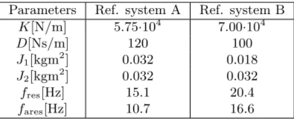
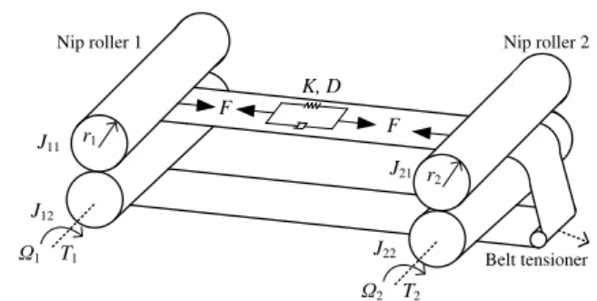
In this paper, an experimental mechanical system with different mechanical configurations is considered to ex-perimentally verify the identification method. The pa-rameters presented in Table1are regarded as the ref-erence system values for the experimental coupled belt drive system under study. First, the proposed identifi-cation method is studied by simulations by considering a closed-loop controlled two-mass system depicted in Figure 2 with both reference system A and B param-eters from Table 1. The dynamics of the mechanical system in Figure 2 can be described by the following set of equations:
J1 dΩ1
dt =T1−Tfr1+r1F (22)
J2 dΩ2
dt =T2−Tfr2−r2F (23)
F=K(r2Ω2−r1Ω1) +D(r2˙Ω2−r1˙Ω1) (24)
Equations (22) and (23) are the elementary dynamic equations for rotation, where J1 = J11 +J12 and J2
Table 1: Parameters of reference systems
Parameters Ref. system A Ref. system B
K[N/m] 5.75·104
7.00·104
D[Ns/m] 120 100
J1[kgm 2
] 0.032 0.018
J2[kgm 2
] 0.032 0.032
fres[Hz] 15.1 20.4
K, D
J21
T1
Ω1
J12
T2
Ω2
J22
J11
Belt tensioner
F F
r1
r2
Nip roller 2 Nip roller 1
Figure 2: Coupled belt system consisting of nip rollers coupled by a flexible belt. A belt tensioner is used to set the tension in the system. The inertia ratio of the system can be adjusted by removing the upper rollers.
= J21 + J22 represents the total moment of inertias
of the nip rollers 1 and 2, Ω1 and Ω2 are the angular
velocities of the rollers,Tis the torque,Tfr is the
fric-tional torque component, ris the roller radius, and F
represents the tension force. The dynamics of the cou-pling is expressed by Eq. (24), where K is the spring constant, and D is the damping constant of the belt material. A more detailed discussion on the mechan-ical system considered in this paper can be found in (Nevaranta et al.,2015b).
The identification experiments are carried out so that the nip roller 2 is treated as a driven one, and the nip roller 1 is used as a load to set the tension of the belt. The angular velocity Ω2 of the nip roller 2 is
controlled with a PI-controller, whereas the nip roller 1 is controlled by a torque controller. Thus, the system is operated at the desired constant nonzero velocity, and the identification is carried out so that the exci-tation signal is added to the torque reference signal of nip roller 2 after the system has been stabilized to the desired velocity. The signals used in the identification are the torque input u(k) = T2 and angular velocity y(k) = Ω2.
3.2 Frequency Response Estimation
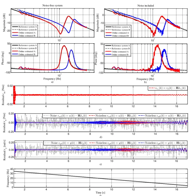
The identification tests are performed so that a con-stant velocity profile 10 rad/s is used, and persistent excitation is superposed to the torque reference. A chirp signal is considered as an excitation signal, which is swept from 35 to 1.5 Hz during 17 s and the ampli-tude is chosen as 1 Nm. The controller C(z) of the system is a low-bandwidth PI-controller with a pro-portional gainKp = 10 1/s and integration timeTi =
0.1 s. The feedback delay of 4 ms is considered in the simulations and assumed to be known in the estimation routine, and the Kalman filter tuning parameter is set
λ= 8. In the simulations, white noise, zero mean, with
a standard deviation 0.1 is added to the output signal
y(k). A direct identification method Eqs. (19)–(21) is considered, where input u(k) and output y(k) signals are used in the identification process. Obviously, the inherent problem of direct identification schemes arises as a result of correlation between the input and out-put signals used in the identification experiment, but as the low bandwidth controller is considered the di-rect identification is applicable for frequency response estimation (Villwock and Pacas, 2008). It is also re-marked that, in practical applications several noise and disturbances sources can be found which influences the frequency response estimation. In this paper, the pro-posed identification method is further validated with an experimental test setup when disturbance sources such as field-bus delays, encoder noise, torque control of the frequency converters and friction influences to the estimation.
101 -20
-10 0
M
ag
n
it
u
d
e
[d
B
]
Noise-free system
Reference system A Reference system B Online estimated A Online estimated B
101 -20
-10 0
M
ag
n
it
u
d
e
[d
B
]
Noise included
Reference system A Reference system B Online estimated A Online estimated B
101 -100
-50 0 50
P
h
as
e
[d
eg
]
Frequency [Hz] a) Reference system A
Reference system B Online estimated A Online estimated B
101 -100
-50 0 50
P
h
as
e
[d
eg
]
Frequency [Hz] b) Reference system A
Reference system B Online estimated A Online estimated B
2 4 6 8 10 12 14 16
-0.02 0 0.02
R
es
id
u
al
ru
[
N
m
]
c)
0ru(k) =ru(k)!Hx^ru(k)
2 4 6 8 10 12 14 16
-0.20 0.00 0.20
R
es
id
u
al
u
[
N
m
]
d)
Noise0uA(k) =u(k)!Hx^u(k) Noiseless0uA(k) =u(k)!Hx^u(k) Noiseless0uB(k) =u(k)!Hx^u(k)
2 4 6 8 10 12 14 16
-0.20 0.00 0.20
R
es
id
u
al
y
[
ra
d
/s
]
e)
Noise0yA(k) =y(k)!Hx^y(k) Noiseless0yA(k) =y(k)!H^xy(k) Noiseless0yB(k) =y(k)!Hx^y(k)
2 4 6 8 10 12 14 16
0 10 20 30 40
F
re
q
u
en
cy
[
H
z]
Time [s] f)
Figure 3: Online directly estimated open loop frequency responses for reference systems A and B a) in the case of a noise-free system and b) when noise is affecting the system output. The tracking properties of the Kalman filter are evaluated with residuals of the signals used in the identification: c) Residual of the excitation signal and estimation. d) Residual of the input signal and estimation. e) Residual of the output signal and estimation. f) Frequency contents of the excitation signal
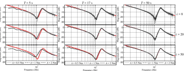
The duration of the sweep and the selection of the Kalman gain is directly related to the tradeoff of the filter tracking and error properties. It is evident that the duration of the identification experiment related to the selection of the Kalman filter tuning parameter has an influence to the accuracy of the frequency re-sponse estimation. In Figure 4 the directly identified frequency responses are shown in the case of reference system A when the Kalman filter tuning parameterλ, the excitation signal amplitude A and duration T of the identification experiment (length of sweep) is
T = 5 s T = 17 s T = 50 s
λ = 8
λ = 20
λ = 50 1 -30 -20 -10 0 M ag n it u d e [d B ] 1 -30 -20 -10 0 M ag n it u d e [d B ] 1 -30 -20 -10 0 M ag n it u d e [d B ] 1 -30 -20 -10 0 M ag n it u d e [d B ] 1 -30 -20 -10 0 M ag n it u d e [d B ] 1 -30 -20 -10 0 M ag n it u d e [d B ] 101 -30 -20 -10 0 M ag n it u d e [d B ] Frequency [Hz]
A = 0.5 Nm A = 1 Nm A = 2 Nm
101 -30 -20 -10 0 M ag n it u d e [d B ] Frequency [Hz]
A = 0.5 Nm A = 1 Nm A = 2 Nm
101 -30 -20 -10 0 M ag n it u d e [d B ] Frequency [Hz]
A = 0.5 Nm A = 1 Nm A = 2 Nm
Figure 4: Online identified open loop frequency responses when the Kalman filter tuning parameter λ and amplitudeA of the excitation signal and duration Tof the identification experiment is varied. The red solid line represents the reference system A.
measurement in order to reduce errors and obtain ac-curate results, which prolongs the duration of the ex-periment. The proposed method for online frequency response estimation is further validated and discussed in the case of experimental results in Section4.
3.3 Loop-transfer Function
When considering classical robustness margins or per-formance indicators, the controller design usually in-volves determination of parameters such as modulus
Mm, gain Gm and phase Pm margins and cross-over
frequency ωc. In practical applications, it is usually
desirable to determine the frequencies at which a given closed-loop system achieves a certain magnitude or phase. In particular, methods such as relay-experiment (de Arruda and Barros,2003) can be regarded as a kind of frequency domain identification for control methods that utilizes only a few points of the frequency response of the loop transfer function to design, for instance, PID controllers. Similarly, the desired open-loop dy-namics can be online shaped by considering for instance an adaptive structure (Balchen and Lie,1987).
The open-loop transfer function G(jω) can be es-timated with the proposed method on a sample-by-sample basis, which makes it possible to use the pro-posed method to calculate the loop transfer function in a real-time by using the known controllerC(jω) to obtainL(jω). As the online identification method esti-mates instantaneous non-parametric model frequency-by-frequency, it also allows to determine rough esti-mates of Mm, Pm and ωc during the identification
experiment by considering different distances in the Nyquist plot. In this paper, the regions inside the unit
circle of the Nyquist plot are determined as regions I, II, III and IV. Region I is located in the plane defined by the negative imaginary and real axes, and thus, this region determines the behaviour at low frequencies.
If the sweep starts exciting low frequencies, and thus at first, the critical frequencyωc can be determined by
calculating the distance of Nyquist curve to the origin frequency-by-frequency as follows
d1(ω)=|L(jω)|=
p
(0−Re[L(jω)])2+ (0−Im[L(jω)])2
(25) and finding the frequency at which the curve intersects the unit circle, thus|L(jωc)|= 1. After the estimated
Nyquist curve has intersected the unit circle and the curve lies in the region I, the modulus and the phase margin can be roughly determined by estimating the distance of the curve to the critical point (-1,0j) by
d2(ω)=|1+L(jω)|=
p
(−1−Re[L(jω)])2+(0−Im[L(jω)])2
(26) By using the first value of this distance metric,d2(ωc),
the phase margin can be obtained as
Pm= cos−1
d
2(ωc)−2
−2
(27) The modulus margin can be estimated by finding the minimum distance of the curve in region I to the crit-ical point, thus Mm = min
ω |1 +L(j
-1 -0.5 0 0.5 1 -1
-0.5 0 0.5
Im
ag
in
ary
a
x
is
Real axis
c = 2.7 Hz
P m = 63.5° M
m = 0.958
fres = 15.3 Hz
f ares = 10.7 Hz
I II
III IV
Ref. systemLA(j!) On-line est. (noise-free sys.) ^L(j!)
-1 -0.5 0 0.5 1
-1 -0.5 0 0.5
Im
ag
in
ary
a
x
is
Real axis
c = 2.7 Hz
P m = 61.3° M
m = 0.915
f res = 15.5 Hz fares = 10.4 Hz
I II
III IV
Ref. systemLA(j!) On-line est. (noise included) ^L(j!)
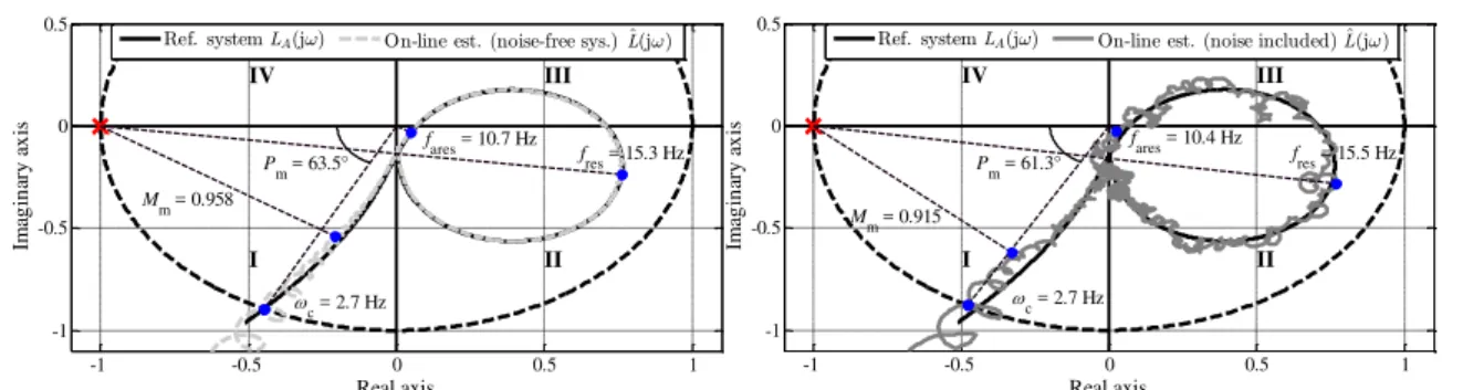
Figure 5: Frequency-by-frequency online-estimated Nyquist curves compared with the reference curve in the case of noise-free system and when the noise is affecting the system output. Equations (25)-(27) are used to determine controller performance parametersMm,Pmandωcin region I. Moreover, the system
parametersωaresandωresin region II are determined by calculating the corresponding distances Eqs.
(25)–(26). The critical point (-1, j·0) is indicated by a red cross.
metrics Eqs. (25)–(26) the anti-resonance ωares and
resonanceωresfrequencies can be determined in region
II similarly as the margins. Hence, the anti-resonance frequency can be estimated in region II by finding the minimum distance to the origind3(ωares) = min
ω
|L(jω)| calculating the distance of the curve similarly as in Eq. (25). Correspondingly, the resonance frequency can be estimated by finding the maximum distance of the curve to the critical point d4(ωres) = max
ω
|1 +L(jω)| similarly as in Eq. (26).
In the Figure 5 the sample-by-sample online-estimated Nyquist curve is shown with the distance metrics Eqs. (26)–(25) that are used to calculate con-troller performance- and system-related parameters in the case of reference system A. The closed-loop con-troller has been designed so that Pm = 63.5◦ and fc = 2.7 Hz. Evidently, in the noise-free case the
online-identified Nyquist curve is in a good correspon-dence with the reference loop transfer function, al-though small discrepancies can be noticed. The be-haviour of the low frequencies is similar with the results in the Figure 3, which further shows that the largest estimation error is in the low frequency band, as ex-pected. It is clear that this is partially due to the start of the chirp excitation, which causes a transient that can also be noticed from the Figure 3 at t = 5 s af-ter the initialization. Naturally, the duration of the sweep and the selection of the Kalman gain have an effect on the frequency response estimation. For this purpose, the known limitation of Kalman filter is the tracking and error tradeoff based on the choice of the Kalman filter tuning parameter λ. Thus, choosing a value of the tuning parameter λfor the Kalman filter is a case-specific compromise, similarly as reported in (Kshirsagar et al.,2016).
In this paper, the rough control performance esti-mates in region I are only considered for illustrative
purposes and to further demonstrate the possibilities of the identification method. It can be seen that the on-line estimated controller-behaviour-related parameters are close to the actual ones; nevertheless, it is pointed out that especially an erroneous estimate of the cross-pointfcdirectly influences to the estimate ofPmas can
be noticed in the noisy case. It is clear that the em-phasized estimation error in the low-frequency region influences these estimates. When considering the dis-tances in region II, the estimated system parameters
faresandfrescorrespond well with the ones of reference
model A illustrated in Table1in the case of both sim-ulations. The estimation of these values are further discussed in Section4.
For actual performance monitoring purposes, it could be more preferable to use a separate soft con-troller to perform the identification experiments in order to analyse the desired controller performance in region I. In practice, the proposed online distance metrics can be used for diagnostics purposes for in-stance by considering a predetermined safety limits in region I. Moreover, the loop-transfer function could be estimated directly from the closed-loop experiment (Barkley and Santi, 2009), (Bhardwaj et al., 2016). These issues will be considered in the future research, and thus not further discussed in this work, where the main focus is to analyse and validate the feasibility of the proposed method for frequency response estima-tion.
4 Experimental Results
programmable logic controller (PLC) is used for data acquisition and to implement the excitation signals, PI controller, and references. It is pointed out that now the experimental system includes a belt-tensioner, which, in practice, changes the system dynamics over to a three-mass-system. However, in this paper, the frequency region around the dominant resonance fre-quency is considered in the online identification, which usually sufficiently reflects dominant behaviour of the real system. The tests are performed so that the same PI-controller parameters are considered as in the sim-ulations, and also the chirp excitation signal is kept same, thus swept from 35 Hz to 1.5 Hz during s 17 s interval. In addition, to further verify the online iden-tification method, the system dynamics of the experi-mental test setup is varied by changing the belt mate-rial and the inertia ratio of the system from 1 to 0.56. The results in Figure8have been obtained by using an experimentally chosen Kalman filter tuning parameter
λ= 8.
Moreover, in order to validate the rough online es-timates of the anti-resonance fares and resonance fres
the experimental system is offline identified by consid-ering the open-loop identification method proposed in (Villwock and Pacas,2008). A PRBS is used to excite the system, and the experimental frequency response estimate Ge(jω) is obtained by Welch method. Then,
the calculation of the mechanical parameters of the an-alytical frequency response function Gmodel(jω) of the
reference two-mass system is accomplished on the ba-sis of the M frequency response data points, and the best fit is iteratively searched by minimizing the error function
J(ϑ) =
M
X
i=1
|Ge(jωi)−Gmodel(jωi,ϑ)|2 (28)
where Ge(jωi) are the experimental frequency
re-sponse data andGmodel(jωi,ϑ) is the analytical model
function with the parameter vector ϑ= [J1,J2,K,D]. In the parameter estimation, the reference model
pa-T1 Ω1
M2 M1
PLC
Speed encoder
Frequency converter
Frequency converter Speed
encoder
400 V 50 Hz
Loading motor
Ω2
T2
Driving motor
400 V 50 Hz
Nip roller 1 Nip roller 2
Belt coupling
Figure 6: Electromechanical system used for experi-mental verification.
rameters of Table1are used in the initialization, thus in the first iteration.
The offline identification experiments are carried out so that the PRBS is generated by a seventeen-cell shift register with values 2.1 Nm and -2.1 Nm (the rated torque being 11.55 Nm). The sampling of the data acquisition is set to 2 ms. In Figure 7, the online-estimated frequency responses are compared with the offline post-processed ones for both system configura-tions: a) reference system A and b) reference system B, respectively. Moreover, the offline post-processed fre-quency responses are compared to the ones calculated by using the identified parameters Eq. (28).
The characteristics of the three-mass-system are clearly visible in the offline frequency responses, and when the mechanical configuration is changed over from reference system A to B, the change of the first resonance is evident. This change can also be seen in the online-estimated frequency response results. The obtained results clearly show a similar behaviour, and the dynamics of two-mass system are seen in the online-estimated amplitude and phase responses in the se-lected band of frequencies. Again, it is worth remark-ing that the offline post-processed frequency response is estimated applying the whole data of the identifi-cation experiment using the PRBS excitation signal, and correspondingly, the online ones are obtained on a sample-by-sample basis from the swept excitation; and thus, these results are not directly comparable. Nev-ertheless, the offline- and online estimated frequency responses are in a good agreement, which clearly in-dicates that the proposed identification method yields accurate results.
With the results of the parameter-fitting for the cor-responding mechanical parameters, the resonance and the anti-resonance frequencies of the two-mass system approximation can be calculated. In Table 2, the es-timated mechanical parameters for the both experi-mental system configurations are shown. The system change can also be seen in the estimated parameters, and especially, the effect of the change in the inertia ra-tio as the resonance and anti-resonance of the system changes. It should be noted that a two-mass-system parameter-fitting is considered for the offline identified frequency responses that have three-mass system char-acteristics, and thus, the mechanical parameter esti-mation results cannot be directly compared to the ini-tial assumption of the system dynamics. However, the offline-estimated resonances ˆfres and anti-resonances
ˆ
fares are used as benchmark values to validate online
estimated ones.
a)
b)
101 102
-30 -20 -10 0
M
ag
n
it
u
d
e
[d
B
]
Frequency [Hz]
Off-line freq. resp. (PRBS) Model from ident. pars. eq. (28) On-line freq. resp. (Chirp)
101 102
-100 -50 0 50
P
h
as
e
[d
eg
]
Frequency [Hz]
Off-line freq. resp. (PRBS) Model from ident. pars. eq. (28) On-line freq. resp. (Chirp)
101 102
-20 -10 0
M
ag
n
it
u
d
e
[d
B
]
Frequency [Hz]
Off-line freq. resp. (PRBS) Model from ident. pars. eq. (28) On-line freq. resp. (Chirp)
101 102
-100 -50 0
P
h
as
e
[d
eg
]
Frequency [Hz]
Off-line freq. resp. (PRBS) Model from ident. pars. eq. (28) On-line freq. resp. (Chirp)
Figure 7: Online-estimated frequency responses Eqs. (20)-(21) compared with the offline post-processed fre-quency response Eq. (1) by using signalsu(k) andy(k) in the identification. a) Experimental system configuration correspond to reference system A and b) reference system B, respectively.
-1 -0.5 0 0.5 1
-1 -0.5 0
Im
ag
in
ary
a
x
is
Real axis
f c = 2.5 Hz P
m = 68.6° M
m = 0.955
f res = 16.8 Hz fares = 12.7 Hz
I II
III
IV On-line ^LA(j!) O,-line ^LA(j!)
-1 -0.5 0 0.5 1
-1 -0.5 0
Im
ag
in
ary
a
x
is
Real axis
f c = 3.2 Hz P
m = 71.0° M
m = 0.956
f res = 19.7 Hz fares = 16.2 Hz
I II
III
IV On-line ^LB(j!) O,-line ^LB(j!)
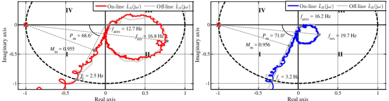
Figure 8: Online-estimated Nyquist curve compared with the offline post-processed one. The system is changed over from reference system A (left Fig.) to B (right Fig.) and equations (25)–(27) are used to determine controller performance parametersMm,Pm andfc in region I. Moreover, the system parametersfares
metrics are used to calculate the controller performance and system parameters. Evidently, the offline- and online-identified Nyquist curves are in a good corre-spondence although small discrepancies can be noticed. Moreover, the system change can be clearly noticed as the size of the resonance loop changes. It should be noted, that the distance metrics in region I are prob-lematic as the largest estimation error is expected in the low frequency region, and the estimated values can be only used as rough estimates of the controller perfor-mance during the identification experiment. Again, it is pointed out that these values are considered for illus-trative purposes only in order to further demonstrate the prospects of the proposed identification method. When focusing on the online-estimated resonance and anti-resonance values in Figure 8, it can be noticed that these values are close to the offline-estimated ones shown in Table 2, thus indicating that instantaneous estimates give reasonable results.
In Figure8it is clear that, the duration of the sweep and the selection of the Kalman gain has an effect on the frequency response estimation. In order to further validate the online-estimated results, the experimental system configuration B is identified using three differ-ent experimdiffer-ental data sets, and the proposed distance metrics are tested by varying the Kalman filter tun-ing parameter. In Figure 9, the estimated values ob-tained from the identification experiments are shown as a function α. It can be seen that similar values of
fres and fares can be estimated by using different val-ues in the Kalman filter gain. Obviously, this result also depends on the amplitude chosen for the excita-tion signal, which is related to the signal-to-noise ratio, but it clearly shows instantaneous values can be used to obtain reasonable estimates. This can be also no-ticed from the minimum distance estimation to critical point. Thus, these results indicate that the proposed online identification method can be used for diagnostics purposes for instance by considering different fault clas-sifiers and/or combination rules. Moreover, the results show the problem of the low-frequency region identifi-cation as a larger deviation in the estimatedPmandfc
parameters can be noticed. These values do not
explic-Table 2: Offline-estimated parameters for different sys-tem configurations
Parameters System conf. A System conf. B
ˆ
K[N/m] 7.51·104
8.70·104 ˆ
D[Ns/m] 140.1 92.7
ˆ
J1[kgm 2
] 0.036 0.037
ˆ
J2[kgm 2
] 0.033 0.016
ˆ
fres[Hz] 17.5 20.1
ˆ
fares[Hz] 12.7 16.7
0 0.1 0.2 0.3 0.4 0.5 0.6 0.7 0.8 0.9 1 16
18 20
F
re
q
u
en
cy
[H
z]
Data set 1
Data set 2 Data set 3
fres fares
0 0.1 0.2 0.3 0.4 0.5 0.6 0.7 0.8 0.9 1 3.1
3.2 3.3 3.4 3.5
fc
[H
z]
b)
Data set 1 Data set 2 Data set 3
0 0.1 0.2 0.3 0.4 0.5 0.6 0.7 0.8 0.9 1 68
70 72 74
P
M
[
°]
Data set 1 Data set 2 Data set 3
0 0.1 0.2 0.3 0.4 0.5 0.6 0.7 0.8 0.9 1 0.94
0.95 0.96 0.97
M
in
.
d
is
t.
t
o
(0
,-j
)
Data set 1 Data set 2 Data set 3
Figure 9: Estimated system and performance parame-ters as a function of the Kalman filter tuning parameter α(r = 1). Data sets 1–2 include chirp with f0 = 35 Hz to f0 = 1.5 Hz and a
data set 3 f0 = 50 Hz to f0= 1.5 Hz during
17 s.
itly describe controller-performance-related behaviour. However, as shown in (Ferretti et al., 2003), a rough estimate offccan be obtained similarly during the
com-missioning state of a PID-controlled two-mass system by using a chirp excitation signal, and successfully used for controller design validation.
4.1 Supporting results and discussion
The main objective of this paper is to propose a nonparametric online frequency response estimation method that is suitable for tracking of a selected band of frequencies, with a specific objective to identify a predefined frequency band around the first resonance frequency of the system. Figure 7 shows that the offline-identified frequency response clearly indicates a three-mass system dynamics.
101 102 -30
-20 -10 0
M
ag
n
it
u
d
e
[d
B
]
Frequency [Hz]
Off-line (PRBS) On-line (Chirp 35 Hz to 1.5 Hz) On-line (Chirp 100 Hz to 1.5 Hz)
101 102
-100 -50 0 50
P
h
as
e
[d
eg
]
Frequency [Hz]
Off-line (PRBS) On-line (Chirp 35 Hz to 1.5 Hz) On-line (Chirp 100 Hz to 1.5 Hz)
Figure 10: Online-estimated frequency responses com-pared with the offline post-processed fre-quency response. The Kalman filter tuning parameter is setλ= 8.
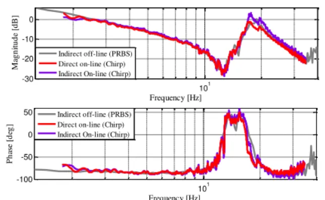
As discussed in Section 2, the open-loop transfer function can be estimated indirectly from a closed-loop identification experiment by using the excitation sig-nal and the output sigsig-nal in the identification routine and by considering the relation of the signals Eq. (5). In Figure 11, the indirectly estimated open-loop of-fline and online frequency responses are shown. The results confirm the remarks in previous results about the good correspondence between the off-line and on-line estimated frequency responses. More importantly, by comparing the directly and indirectly obtained re-sults in Figures 11, it can be seen that the obtained open-loop models are rather similar with only minor noticeable differences. These results clearly indicate that the proposed non-parametric online identification routine supports the well-established frequency domain closed-loop identification theories (Heath, 2001), and thus, can be applied accordingly to determine the open-loop frequency response from closed-open-loop experiments. Furthermore, in the case of indirect identification, the proposed method gives more design freedom in the parametrization of Kalman filter as the excitation sig-nal used in the identification is known in advance.
In this paper, the experimental results clearly val-idate the proposed methodology and effectiveness of using online Kalman filters for frequency response anal-ysis. The known limitation of the Kalman filter is its convergence time and tracking tradeoff with respect on the choice of tuning parameters. This limitation requires the frequency sweep to be slow. However, usually in the case of chirp-excitation-based identifi-cation, the duration of the sweep must be designed long in order to reduce errors and obtain accurate re-sults (Ostring et al.¨ ,2001). A second drawback can be found when considering identification of systems with nonlinear dynamics. The chirp signal can have a
dis-101 -30
-20 -10 0
M
ag
n
it
u
d
e
[d
B
]
Frequency [Hz]
Indirect off-line (PRBS) Direct on-line (Chirp) Indirect On-line (Chirp)
101 -100
-50 0 50
P
h
as
e
[d
eg
]
Frequency [Hz]
Indirect off-line (PRBS) Direct on-line (Chirp) Indirect On-line (Chirp)
Figure 11: Indirectly estimated online frequency re-sponse compared to the offline post-processed frequency response Eq. (6) by using the signalsru(k) andy(k) and known
controllerG(z) in the identification. The di-rectly online-estimated frequency response is also shown.
turbing effect, because a number of other spectral lines are also excited with the frequency lines of interest. De-spite these limitations, the chirp-excitation-based of-fline identification is widely applied for instance to the identification of the flexibilities of nonlinear industrial robot manipulators (Ostring et al.¨ ,2003), (Saupe and Knoblach,2015).
5 Conclusions
This paper presented an online non-parametric ap-proach that is based on a time-frequency presentation of signals in order to estimate a frequency response of a closed-loop controlled servomechanism in a compu-tationally efficient manner. The method is based on a fixed-coefficient non-parametric Kalman filter, which is updated with the known frequency of the chirp exci-tation signal. The results from the simulations and ex-perimental tests show that the approach can be used to achieve reasonable estimates of the frequency responses in real time on a sample-by-sample basis. The online estimated frequency responses during operation were compared with the corresponding frequency responses obtained by off-line identification using the whole data of the identification experiment collected prior to the estimation. The results show acceptable agreement, thus indicating that the proposed method is suitable for the online frequency-domain nonparametric iden-tification of a mechanical system. Moreover, it was experimentally validated that the method is feasible to detect system changes for diagnostics purposes.
dynam-ics may lead to the degradation of the control perfor-mance or cause unexpected interruptions, it is impor-tant to detect the system changes as proactive main-tenance before they lead to performance degradation. The future work will focus on the performance assess-ment and diagnostics opportunities of the identification method and the option to diagnose mechanical faults e.g. changes in the resonances resulting from deterio-ration.
References
de Arruda, G. and Barros, P. Relay-based closed loop trasfer function frequency points estimation.
Au-tomatica, 2003. 39(2):309–315. doi:
10.1016/S0005-1098(02)00205-4.
Balchen, J. and Lie, B. An adaptive controller based upon continous estimation of the closed loop fre-quency response. Modeling, Identification and Con-trol, 1987. 8(4):223–240. doi:10.4173/mic.1987.4.3. Barkley, A. and Santi, E. Improved online
iden-tification of a dc-dc converter and its control loop gain using cross-correlation methods. IEEE
Trans. on Power. Elect., 2009. 24(8):2021–2031.
doi:10.1109/TPEL.2009.2020588.
Beineke, S., Wertz, H., Sch¨utte, F., Grotstollen, H., and Fr¨ohleke, N. Identification of nonlinear two-mass systems for self-commissioning speed control of elec-trical drives. in Proc. IEEE IECON, 1998. pages 2251–2256. doi:10.1109/IECON.1998.724071. Bhardwaj, M., Choudhury, S., Poley, R., and Akin,
B. Online frequency response analysis: A powe-ful plug-in tool for compensation design and health assessment of digitally controlled power controllers.
IEEE Trans. Ind. Appl., 2016. 00(99):1–10.
doi:0.1109/TIA.2016.2522951.
Bitmead, R., Tsoi, A. C., and Parker, P. J. A kalman filtering approach to short-time fourier analysis.
IEEE Trans. Acoust., Speech, Signal Process, 1986.
34(6):1493–1501. doi:10.1109/TASSP.1986.1164989. Bittanti, S. and Savaresi, S. M. On the parame-terization and design of an extended kalman filter frequency tracker. EEE Trans. Aut. Cont.), 2000. 45(9):1718–1724. doi:10.1109/9.880631.
Duda, K. Accurate, guaranteed stable, slid-ing discrete fourier transform. IEEE
Sig-nal Processing Magazine,, 2010. 27(6):124–127.
doi:10.1109/MSP.2010.938088.
Ferretti, G., Magnani, G., and Rocco, P. Load be-havior concerned pid control for two-mass servo systems. In Proc. of IEEE/ASEM Int. Conf. on
Adv. Intelligent Mechatronics, 2003. pages 821–826.
doi:10.1109/AIM.2003.1225448.
Goubej, M. Kalman filter based observer design for real-time frequency identification in motion control systems. in Proc. 20th Conf. on Process Control, 2015. pages 296–301. doi:10.1109/PC.2015.7169979. Goubej, M., Krejˇc´ı, A., and Schlegel, M. Robust fre-quency identification of oscillatory electromechani-cal systems. in Proc. 18th Conf. on Process Control, 2013. pages 79–84. doi:10.1109/PC.2013.6581387. Heath, W. Bias of indirect non-parametric transfer
function estimates for plants in closed loop.
Auto-matica, 2001. 37(10):1529–1540. doi:
10.1016/S0005-1098(01)00105-48.
Holzel, M. and Morelli, E. Real-time frequency re-sponse estimation from flight data. in Proc. AIAA
Atmospheric Flight Mechanics Conference, 2011.
pages 1–26. doi:10.2514/6.2011-6358.
Jenssen, A. and Zarrop, M. Frequency domain change detection in closed loop. in Proc. Int. Conf. in Con-trol, 1994. pages 676–680. doi:10.1049/cp:19940213. Kamwa, I., Samantaray, S. R., and Joos, G. Wide fre-quency range adaptive phasor and frefre-quency pmu al-gorithms.IEEE Trans. Smart Grid., 2014. 5(2):569– 579. doi:10.1109/TSG.2013.2264536.
Kshirsagar, P., Juang, D., and Zhang, Z. Implemen-tation and evaluation of online system identifica-tion of electromechanical systems using adaptive fil-ters. IEEE Trans. Ind. Appl., 2016. 00(99):1–9. doi:10.1109/TIA.2016.2515994.
Kurita, Y., Hashimoto, T., and Ishida, Y. An ap-plication of time delay estimation by anns to fre-quency domain i-pd controller. in Proc. Int. Joint
Conf. on Neural Networks, 1999. pages 2164–2167.
doi:10.1109/IJCNN.1999.832723.
LaMaire, R., Valavani, L., Athans, M., and Gunter, S. A frequency-domain estimator for use in adaptive control systems. in Proc. American Control Conf., 1987. pages 238–244.
Ljung, L. Perspectives on system identification.
Annual Reviews in Control, 2010. 34(1):1–12.
doi:10.1016/j.arcontrol.2009.12.001.
O., and Pyrh¨onen, J. Online identification of a me-chanical system in frequency domain using sliding
dft. IEEE Trans. Ind. Electron., 2016. 63(9):5712–
5723. doi:10.1109/TIE.2016.2574303.
Nevaranta, N., Parkkinen, J., Niemel¨a, M., Lindh, T., Pyrh¨onen, O., and Pyrh¨onen, J. Recursive identifica-tion of linear tooth belt-drive system.in Proc. EPE, 2014. pages 1–8. doi:10.1109/EPE.2014.6910904. Nevaranta, N., Parkkinen, J., Niemel¨a, M., Lindh, T.,
Pyrh¨onen, O., and Pyrh¨onen, J. Online estima-tion of linear tooth-belt drive system parameters.
IEEE Trans. Ind. Electron, 2015a. 62(11):7214–
7223. doi:10.1109/TIE.2015.2432103.
Nevaranta, N., Parkkinen, J., Niemel¨a, M., Lindh, T., Pyrh¨onen, O., and Pyrh¨onen, J. Online Identification of a Mechanical System in the Fre-quency Domain with Short-Time DFT. Modeling,
Identification and Control, 2015b. 36(3):157–165.
doi:10.4173/mic.2015.3.3.
Olivier, P. D. Online system identification using la-guerre series. in Proc. IEE Control Theory and
Application, 1994. 141(4):249–254. doi:
10.1049/ip-cta:19941239. ¨
Ostring, M., Gunnarsson, S., and Norrl¨of, M. Closed loop identification of the physical parameters of an industrial robot. In Proc. of 32th Int. Symp. on
Robotics, 2001. pages 1–20.
¨
Ostring, M., Gunnarsson, S., and Norrl¨of, M. Closed-loop identification of an industrial robot contain-ing flexibilities. Control Engineering Practice, 2003. 11(3):291–300. doi:10.1016/S0967-0661(02)00114-4. Parker, P. and Bitmead, R. Adaptive frequency
response identification. in Proc. 28th Conf. on
Decision and Control, 1987. pages 348–353.
doi:10.1109/CDC.1987.272820.
Perdomo, M., Pacas, M., Eutebach, T., and Immel, J. Identification of variable mechanical parameters us-ing extended kalman filters. in 9th IEEE Int. Symp.
on Diagnostics for Electric Machines, Power
Elec-tronics and Drives (SPEMPED), 2013. pages 377–
383. doi:10.1109/DEMPED.2013.6645743.
Saarakkala, S. and Hinkkanen, M. Identifica-tion of two-mass mechanical systems using torque excitation: Design and experimental evaluation.
IEEE Trans. Ind. Appl., 2015. 51(5):4180–4189.
doi:10.1109/TIA.2015.2416128.
Saupe, F. and Knoblach, A. Experimental de-termination of frequency response function es-timates for flexible joint industrial manipula-tors with serial kinematics. Mechanical
Sys-tems and Signal Processing, 2015. 52(4):60–72.
doi:10.1016/j.ymssp.2014.08.011.
Schoukens, J., Pintelon, R., and Rolain, Y. Broadband versus stepped sine frf measurements.
IEEE Trans. Instr. Meas., 2000. 49(1):275–278.
doi:10.1109/19.843063.
Schoukens, J., Vandersteen, G., Rolain, Y., and Pin-telon, R. Frequency response function measurements using concatenated subrecords with arbitrary length.
IEEE Trans. Instr. Meas., 2012. 61(10):2682–2688.
doi:10.1109/TIM.2012.2196400.
Schutte, F., Beineke, S., Rolfsmeir, A., and Grot-stollen, H. Online identification of mechanical pa-rameters using extended kalman filters. in Conf.
Rec. IEEE-IAS Annual Meeting, 1997. pages 501–
508. doi:10.1109/IAS.1997.643069.
Villwock, S. and Pacas, M. Application of the welch-method for the identification of two- and three-mass-systems. IEEE Trans. Ind. Electron, 2008. 55(1):457–466. doi:10.1109/TIE.2007.909753. Yen, G. G. Frequency-domain vibration control
us-ing adaptive neural network. in Proc. Int. Joint
Conf. on Neural Networks, 1997. pages 806–810.