Spatial pattern analysis of landslide using landscape metrics and logistic regression: a case study in Central Taiwan

(1)

HESSD

7, 3423–3451, 2010

Spatial pattern analysis of landslide

using metrics and logistic regression

Y.-P. Lin et al.

Title Page

Abstract Introduction

Conclusions References

Tables Figures

◭ ◮

Back Close

Full Screen / Esc

Printer-friendly Version

Interactive Discussion

Discussion

P

a

per

|

Dis

cussion

P

a

per

|

Discussion

P

a

per

|

Discussio

n

P

a

per

|

Hydrol. Earth Syst. Sci. Discuss., 7, 3423–3451, 2010 www.hydrol-earth-syst-sci-discuss.net/7/3423/2010/ doi:10.5194/hessd-7-3423-2010

Hydrology and Earth System Sciences Discussions

This discussion paper is/has been under review for the journal Hydrology and Earth System Sciences (HESS). Please refer to the corresponding final paper in HESS if available.

Spatial pattern analysis of landslide using

landscape metrics and logistic

regression: a case study in Central

Taiwan

Y.-P. Lin1, H.-J. Chu1, and C.-F. Wu2

1

Department of Bioenvironmental Systems Engineering, National Taiwan University, 1, Sec. 4, Roosevelt Rd., Da-an District, Taipei City 106, Taiwan, China

2

Department of Horticulture, National Chun Hsing University, 250, Kuo Kuang Rd., Taichung 402, Taiwan, China

Received: 21 May 2010 – Accepted: 29 May 2010 – Published: 11 June 2010

Correspondence to: H.-J. Chu (honejaychu@gmail.com)

(2)

HESSD

7, 3423–3451, 2010

Y.-P. Lin et al.

Title Page

Tables Figures

◭ ◮

Back Close

Full Screen / Esc

Discussion

P

a

per

|

Dis

cussion

P

a

per

|

Discussion

P

a

per

|

Discussio

n

P

a

per

|

Abstract

The Chi-Chi Earthquake of September 1999 in Central Taiwan registered a moment magnitude MW of 7.6 on the Richter scale, causing widespread landslides. Subse-quent typhoons associated with heavy rainfalls triggered the landslides. The study investigates multi-temporal landslide images from spatial analysis between 1996 and

5

2005 in the Chenyulan Watershed, Taiwan. Spatial patterns in various landslide fre-quencies were detected using landscapes metrics. The logistic regression results indi-cate that frequency of occurrence is an important factor in assessing landslide hazards. Low-occurrence landslides sprawl the catchment while the sustained (frequent) land-slide areas cluster near the ridge as well as the stream course. From those results,

10

we can infer that landslide area and mean size for each landslide correlates with the frequency of occurrence. Although negatively correlated with frequency in the low-occurrence landslide, the mean size of each landslide is positively related to frequency in the high-occurrence one. Moreover, this study determines the spatial susceptibilities in landslides by performing logistic regression analysis. Results of this study

demon-15

strate that the factors such as elevation, slope, lithology, and vegetation cover are sig-nificant explanatory variables. In addition to the various frequencies, the relationships between driving factors and landslide susceptibility in the study area are quantified as well.

1 Introduction

20

Landslides are major hazards and have a wide range of impact on geomorphic pro-cesses and erosion patterns (Glade, 2003; Page et al., 1994; Remondo et al., 2005). Spatial patterns in landslides are the result of an interaction among dynamic processes operating across abroad range of spatial and temporal scales. External forces (i.e. typhoons with torrential rainfall and earthquakes) and human activity (i.e. land-use

25

(3)

HESSD

7, 3423–3451, 2010

Y.-P. Lin et al.

Title Page

Tables Figures

◭ ◮

Back Close

Full Screen / Esc

Discussion

P

a

per

|

Dis

cussion

P

a

per

|

Discussion

P

a

per

|

Discussio

n

P

a

per

|

et al., 2005). In addition, the landslides after major disturbances such as an earthquake may be easily triggered by subsequent typhoons associated with heavy rainfalls. After the 1999 Chi-Chi earthquake (ML₌7.6 on the Richter scale), the landslides tend to in-crease in both number and magnitude in Central Taiwan (Chen et al., 2005; Chen and Wu, 2006; Galewsky et al., 2006; Lin et al., 2008c).

5

Delineating areas susceptible to landslides is essential for land-use activities and hazard management in the area. We always concern about where landslides will occur, how frequent they will occur, and how large they will be (Guzzetti et al., 2005).

To mitigate hazards, deterministic and non-deterministic models have been devel-oped to generate landslide susceptibility maps (Huang and Kao, 2006). Many

re-10

searchers have used logistic regression to predict probabilities of landslide occurrence by analyzing the functional relationships between driving factors and landslides (Ay-alew and Yamagishi, 2005; Can et al., 2005; Chang et al., 2007; Dai and Lee, 2003; den Eeckhaut et al., 2006; Duman et al., 2006; Lee, 2005; Ohlmacher and Davis, 2003; Yesilnacar and Topal, 2005). Landslide susceptibility mapping relies on a rather

com-15

plex knowledge of vegetation condition, slope movements and other local controlling factors. Moreover, the landslide occurrence frequency and spatial susceptibility are important indices to understand the mechanism for managers and engineers. Most landslide areas are new occurrences and some landslides are sequent ones (Lin et al., 2008b). However, the susceptibility of landslide maps depends mostly on the

oc-20

currence number of landslides. The geological and geomorphological properties e_ffect landslide inventories at the sites with the occurrence frequency. Based on landslide occurrence, the landslide patterns are classified into various levels. In each level, the relationships between landslides and driving factors will be identified specifically.

In the study, landscape metrics have proved e_ffective landslide assessment because

25

(4)

HESSD

7, 3423–3451, 2010

Y.-P. Lin et al.

Title Page

Tables Figures

◭ ◮

Back Close

Full Screen / Esc

Discussion

P

a

per

|

Dis

cussion

P

a

per

|

Discussion

P

a

per

|

Discussio

n

P

a

per

|

the number, area, composition, configuration, and connectivity of various patch types. Landslide composition refers to the characteristics associated with the variety and abundance of patch types within a given landscape. Spatial configuration of a land-slide denotes the spatial characteristics and arrangement, position, or orientation of patches within a landslide class. In addition, the major disturbances a_ffected the

iso-5

lation, size, and shape complexity of patches at the landscape levels. Disturbances of various types, sizes, and intensities, following various tracks, have various e_ffects on the landslide patterns and variations of the Chenyulan watershed (Lin et al., 2006).

In the study, the landslides data derived from SPOT satellite images before and after the Chi-Chi earthquake in the Chenyulan basin of Taiwan, as well as multiple images

af-10

ter large typhoons such as typhoon Herb, Xangsane, Toraji, Dujuan and Mindulle were analyzed for landslide identification. The study identifies the various spatial occurrence patterns of landslides caused by disturbances using landscape metrics. Besides, this study clarifies the relationships between the driving factors and the landslides with var-ious occurrence frequencies using logistic regression. Results provide the information

15

to understand spatial structures of landslide within the occurrence frequencies for the hazard management.

2 Material and methods

2.1 Study area

The Chenyulan watershed, located in Central Taiwan, is a classical intermountain

wa-20

tershed which is traversed by the Chenyulan stream in the south to north direction. The area of this watershed is 449 km2. Most parts of the watershed are over 1000 m in elevation (i.e. the average elevation is 1591 m). The Chenyulan stream had a gra-dient of 6.1%, and more than 60% of its tributaries had gragra-dients exceeding 20% (Lin et al., 2004; Lin et al., 2006). Di_fferences in uplifting along the fault generated

abun-25

(5)

HESSD

7, 3423–3451, 2010

Y.-P. Lin et al.

Title Page

Tables Figures

◭ ◮

Back Close

Full Screen / Esc

Discussion

P

a

per

|

Dis

cussion

P

a

per

|

Discussion

P

a

per

|

Discussio

n

P

a

per

|

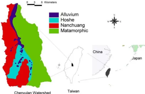
dominant lithologies in the metamorphic terrains. Based on the relative amounts of slate and meta-sandstone, the metamorphic strata in the eastern part of the study area are divided into four parts: Shihpachuangchi, Tachien Meta-Sandstone, Paileng Meta-Sandstone, and Shuichangliu (Lin et al., 2004, 2006). The major formations west of Chenyulan catchment are Nanchuang Formation, Hoshe Formation and Alluvium

5

(Fig. 1). Shale and cemented sandstone are the major lithologies in the region (Lin et al., 2008a). Furthermore, the 1999 Chi-Chi earthquake at 23.85◦_{N, 120.81}◦_{E, with}

a focal depth of 8.0 km, was triggered by reactivation of the Chelungpu fault in Central Taiwan on September 21, 1999. The earthquake caused 2400 deaths, 8373 casual-ties, and over US$ 10 billion in damages (Lin et al., 2004). After a strong earthquake,

10

the number and magnitude of the landslides increase in the study area (Chen et al., 2005; Chen and Wu, 2006; Galewsky et al., 2006; Lin et al., 2008c).

Landslides are susceptible to being triggered by the combined e_ffects of steep to-pography, weak geological formations, and vegetation condition (Chang et al., 2007; Dai and Lee, 2003; Lee, 2005). In the study, lithology, wetness index, normalized

dif-15

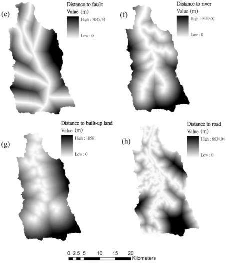
ference vegetation index (NDVI), elevation, slope, distances to fault, river, road and built-up land are used as the driving factors in the model (Fig. 2). These data for the study are raster-based and the cell size is 40 m. The brief introductions are as the following.

(1) Lithology: Previous study ruled out rock strength as one of control on the rate

20

of landsliding in the Chenyulan catchment (Lin et al., 2008b). The landslide densities varied significantly between lithologies (Fig. 1). The rock formations such as Alluvial, Hoshe, and Nanchuang are used for logistic regression, with Metamorphic serving as the reference category in the modeling.

(2) Wetness index: The wetness index combines local upslope contributing area

25

(6)

HESSD

7, 3423–3451, 2010

Y.-P. Lin et al.

Title Page

Tables Figures

◭ ◮

Back Close

Full Screen / Esc

Discussion

P

a

per

|

Dis

cussion

P

a

per

|

Discussion

P

a

per

|

Discussio

n

P

a

per

|

streams. Overall, the range of wetness index is from 3.5 to 22.2 and the mean is 6.4 (Fig. 2a).

(3) NDVI: The NDVI is most widely used vegetation index used to estimate plant biomass through the integration of the red–visible and near-infrared spectral regions to represent plant pigmentation and chlorophyll content, respectively, in the

characteriza-5

tion of land cover conditions (Lin et al., 2009; Walsh et al., 2001; Chu et al., 2009). The NDVI images of the study area were generated from SPOT HRV images with a reso-lution of 20 m. The NDVI in the area on 1996/11/08 ranges are from 0.11 to 0.49 with the mean of 0.36 (Fig. 2b).

(4) Elevation and slope (Fig. 2c and d): The range of elevation is from 304 m to

10

3847 m, gradually decreasing from south to north. In the study area, slopes range from 0◦ _{to 80.6}◦_{, with a mean of 32.9}◦_{. Landslides tend to occur on steeper slopes,}

especially where the slope is covered by a thin colluvium (Chang et al., 2007).

(5) Distance to fault, river, built-up land, and road (Fig. 2e,f): The landslides are significantly related to the distances to fault and river (Lin et al., 2008a). Moreover,

15

the anthropogenic disturbances and impacts such as land-use changes induce the landslide. In the area, distances to built-up land and road are the factors driving land-use changes.

2.2 Landscape metrics

Landscape metrics are particularly promising conceptual and analytical tools in

land-20

scape ecology because they are readily applicable (Leit ˜ao et al., 2006). To assess spatial landslide patterns with the frequencies, this work calculated landscape metrics using the Patch Analyst (Elkie et al., 1999). Landscape metrics were categorized as the area, density, edge, shape, isolation/proximity, contagion, and diversity metrics. This study used the nine landscape indices, namely Class Area (CA), Number of Patches

25

(7)

composi-HESSD

7, 3423–3451, 2010

Y.-P. Lin et al.

Title Page

Tables Figures

◭ ◮

Back Close

Full Screen / Esc

Discussion

P

a

per

|

Dis

cussion

P

a

per

|

Discussion

P

a

per

|

Discussio

n

P

a

per

|

tions and configurations in the watershed (Table 1). Detailed descriptions of the above metrics can be found in McGarigal and Marks (1994) and Elkie et al. (1999).

2.3 Logistic regression

The logistic regression provides the probability of the presence of each landslide at each location based on their drivers (Ayalew and Yamagishi, 2005; Chang et al., 2007;

5

Lee, 2005). The model quantifies the relationships between landslide occurrence and the drivers, and is specified by:

logi t(y_i)₌ln

_P

i

1₋P_i

(1)

and

P_i₌

exp β₀₊ k

P

j=1 β_jx_{j i}

!

1+exp β₀₊ k

P

j=1 β_jx_{j i}

! (2)

10

whereP_i is the probability of a landslide occurring in a grid cell (pixel)i;kis the number of driving factors;y_i is the dependent variable (i.e. landslide occurrence) in a grid cell

i; x_{j i} is the driving factor of each cell i in the driving factor j; β₀ is the estimated coe_fficient; and β_j is the coe_fficient of each driving factor in the logistic model. In the study, landscape metrics are used to clarify the spatial patterns of landslide data into

15

the classifications firstly. Then, the probability maps of landslides based on the various occurrence numbers are generated using logistic regression.

Relative Operating Characteristic (ROC)

The area under the Relative Operating Characteristic (ROC) curve was calculated to measure the explanatory power of logistic regression model (Pearce and Ferrier, 2000).

(8)

HESSD

7, 3423–3451, 2010

Y.-P. Lin et al.

Title Page

Tables Figures

◭ ◮

Back Close

Full Screen / Esc

Discussion

P

a

per

|

Dis

cussion

P

a

per

|

Discussion

P

a

per

|

Discussio

n

P

a

per

|

The ROC curve is constructed by calculating the sensitivity and specificity of the re-sulting landslide for each possible landslide (Carrara et al., 2008; den Eeckhaut et al., 2006; Falaschi et al., 2009). The ROC characteristic is a measure for the goodness of fit of a logistic regression model similar to ther2 statistic in ordinary least square regression. The ROC values above 0.7 are generally considered good while values

5

exceeding 0.9 are considered to indicate an excellent model fit. Since the ROC is con-sidered a proper measure to evaluate the goodness of fit, the ROC is applied to assess the model performance in the study.

3 Results

3.1 Data processing and analysis

10

The eight SPOT satellite images from 1996 to 2005 (i.e. (1) 8 November 1996, (2) 6 March 1999, (3) 31 October 1999, (4) 27 November 2000, (5) 20 November 2001, (6) 17 December 2003, (7) 19 November 2004 and (8) 11 November 2005) were first classified via supervised classification with maximum likelihood and fuzzy methods us-ing ERDAS IMAGINE software, based on 1/25000 black and white aerial photographs

15

and ground truth data (Lin et al., 2006). Subsequently, the classified images and geo-graphical data (roads, buildings, slopes and band ranges) of the watersheds were used to construct the knowledge base in the Knowledge Engineer of IMAGINE software for final SPOT image classification. The IMAGINE user manual presented the theorems underlying the above image classification methods in details. Moreover, kappa values

20

were calculated to assess the classification accuracy (den Eeckhaut et al., 2006). The final accuracy assessment of each SPOT image used 747 pixels, with the accuracy assessment using between 30 and 475 pixels per training class. The accuracy and kappa values exceeded 82% and 0.77, respectively. Eventually, the land cover cat-egories were classified into landslide and non-landslide. Figure 3 demonstrates the

25

(9)

HESSD

7, 3423–3451, 2010

Y.-P. Lin et al.

Title Page

Tables Figures

◭ ◮

Back Close

Full Screen / Esc

Discussion

P

a

per

|

Dis

cussion

P

a

per

|

Discussion

P

a

per

|

Discussio

n

P

a

per

|

1999, (c) 20 November 2001, and (d) 19 November 2004.

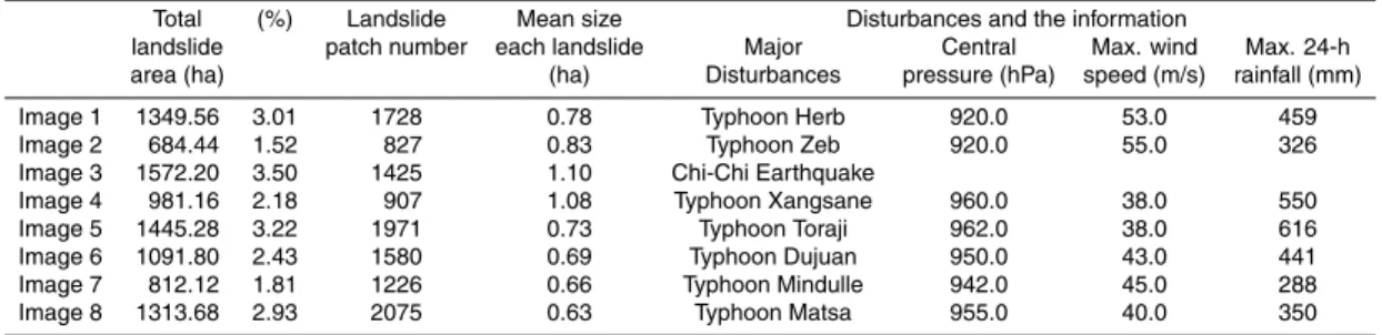
Table 2 lists the landslide number, total landslide area and mean size each land-slide, and typhoon backgrounds such as the typhoon central pressures, maximum wind speeds and the maximum 24-h rainfall at typhoon events. Typhoon Herb in 1996 came before the Chi-Chi earthquake and increased numerous new debris and landslides in

5

the catchment. After the 1999 Chi-Chi earthquake, an area of approximately 1500 ha was a_ffected by landsliding in the basin (Lin et al., 2008a). On 30 July 2001 typhoon Toraji swept across Central Taiwan from east to west, with a maximum wind speed of 38 m/s and a radius of 180 km. The typhoon brought extremely heavy rainfall, from 230 to 650 mm/d, and triggered numerous landslides in Taiwan (Lin et al., 2009). In

10

2004 typhoon Mindulle with maximum wind speed of 45 m/s and a radius of 200 km chronologically produced heavy rainfall that fell across the eastern and central parts of Taiwan.

3.2 Landslide patterns analysis with the frequencies

Figure 4 demonstrates the spatial patterns of landslide frequency (i.e. the occurrence

15

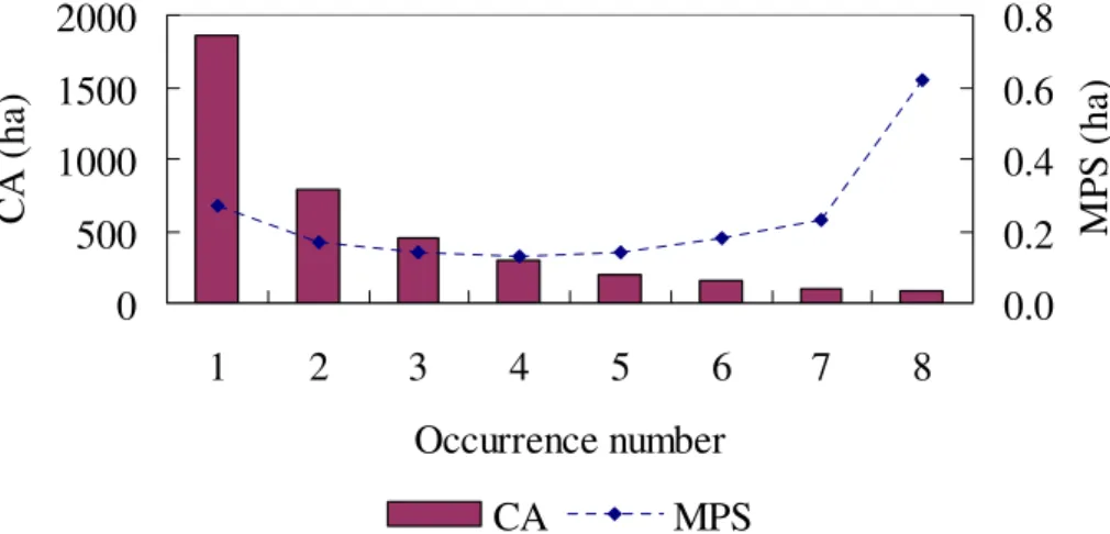
number of landslide at each cell) during ten years based on eight landslide images. If the land cover in the cell is a landslide, then the cell occurrence number will be accumu-lated. Table 3 shows landscape metrics of the landslide occurrence number in Fig. 4. Class Area (CA) results show landslide area is 1866 ha at occurrence number₌1 and 81 ha at occurrence number₌8. The proportion of landslide areas are numerous new

20

occurrences (4.16% of total area at occurrence number₌1) and few sustained land-slides subsequently occur 0.18% of total area at occurrence number₌8. Moreover, the relationships between the Class Area (CA) and Mean Patch Size (MPS) with various landslide occurrence number are shown in Fig. 5. Result shows that Class Area (CA) of landslide declines as the occurrence number increases. Furthermore, the

relation-25

(10)

HESSD

7, 3423–3451, 2010

Y.-P. Lin et al.

Title Page

Tables Figures

◭ ◮

Back Close

Full Screen / Esc

Discussion

P

a

per

|

Dis

cussion

P

a

per

|

Discussion

P

a

per

|

Discussio

n

P

a

per

|

0.62 ha. It is found that the MPS is negatively correlated with the occurrence number in small occurrence number (occurrence number_≤4) landslide but is positively correlated with the occurrence number in large one. The Patch Size Standard Deviation (PSSD) and Patch Size Coefficient of Variance (PSCOV) represent that landslides in the large occurrence number (occurrence number₌7 and 8) contain considerable variability but

5

landslides at occurrence number₌5 reveal the lowest variability (Table 3). The Total Edge (TE) metric is negatively correlated with the occurrence number, hence a longer landslide class edge is in low-occurrence landslides. The Edge Density (ED) presents the patch edge densities become small in occurrence number₌1, 7, and 8. More-over, the landslide patch is nearly squared-shape as the Mean Shape Index (MSI) is

10

close to one. Otherwise, the landslide patch shape is distorted. The shape index (i.e. MSI) shows the overall patch shapes are irregular in lowest and largest occurrence number (i.e. occurrence number₌1 or 7, 8). Furthermore, the Mean Nearest Neighbor (MNN) increases from 43 m to 372 m with the occurrence number increasing. The re-sult implies that landslides are more isolated and less clustered in the high-occurrence

15

landslides.

3.3 Landslide susceptibility map with the frequencies

The logistic regression model was used to estimate the probabilities for landslide class with the low-occurrence landslides (occurrence number_≤4), high-occurrence land-slides (occurrence number>4) and entire landslides (occurrence number>0) between

20

landslides and their driving factors. The low-occurrence and high-occurrence (sus-tained) landslides occupy 7.55% and 1.17% of the total watershed area, respectively. For accurate estimation, the study determines the susceptibility map with the low-occurrence and high-low-occurrence landslides during ten years using logistic regression. Fig. 6 implies the susceptibility map of landslides with various frequencies in the study

25

(11)

HESSD

7, 3423–3451, 2010

Y.-P. Lin et al.

Title Page

Tables Figures

◭ ◮

Back Close

Full Screen / Esc

Discussion

P

a

per

|

Dis

cussion

P

a

per

|

Discussion

P

a

per

|

Discussio

n

P

a

per

|

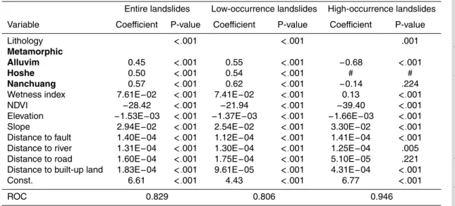
Logistic regression models with low-occurrence and entire landslides with Nagelk-erke R2₌0.21 and 0.29 during ten years are shown in Table 4. Results show both models with low-occurrence and entire landslides are significant at a 0.01 significance level. The finding presents that lithology, wetness index, slope, distance to fault, dis-tance to river, disdis-tance to road and disdis-tance to built-up land are positive coefficient

fac-5

tors; NDVI and elevation are negative coe_fficient factors. Table 4 also represents logis-tic regression model with high-occurrence landslides with NagelkerkeR2₌0.43 during the periods. The fitted logistic model used five positive coefficient factors (i.e. wetness index, slope, the distance to fault, distance to river, and distance to built-up land) and two negative coe_fficient factors (i.e. NDVI and elevation). The results show most

ex-10

planatory variables with high-occurrence landslide are significant at a significance level. However, the lithology and distance to road are not significant explanatory variables. The lithology category data could not be a significant explanatory variable because high-occurrence landslides cluster in the particular areas in Metamorphic and Nam-chung. Accordingly, the models’ ROC values for the entire landslides, low-occurrence,

15

and high-occurrence landslides models are 0.829, 0.806 and 0.946, respectively. The high ROC values indicate the significantly good fit of the model to the observations which may be explained by the capacity of models to capture relationships between driving factors and landslide patterns. Results show high-occurrence landslide model provides the most accurate landslide susceptibility estimation.

20

4 Discussion

4.1 Landslide spatial patterns considering occurrence frequency

Landscape metrics analyses showed that the various frequent landslides produced var-iously fragmented and isolation among landslide patches across the entire Chenyulan watershed (Table 3). Landscape metrics could assess and identify the spatial

pat-25

(12)

HESSD

7, 3423–3451, 2010

Y.-P. Lin et al.

Title Page

Tables Figures

◭ ◮

Back Close

Full Screen / Esc

Discussion

P

a

per

|

Dis

cussion

P

a

per

|

Discussion

P

a

per

|

Discussio

n

P

a

per

|

landslide class area (CA) negatively associates with the occurrence frequency. In addi-tion, mean patch size (MPS) of landslides is associated with the occurrence frequency. MPS of landslide is negatively correlated with frequency in the low occurrence num-ber, but is positively associated with frequency in the others. In addition, the minimum mean patch size and mean shape index of landslides during ten years are under the

5

middle frequency (occurrence number₌4). Moreover, the landslide size variation (i.e. PSSD and PSCOV) is lowest at occurrence number=5. The edge density of land-slide is largest at occurrence number₌5. The landscape metrics (i.e. MPS, ED, MSI, PSSD, and PSCOV) show that there is an inflection point at occurrence number₌4 or 5. Hence, spatial landslide patterns could be classified into low-occurrence (occurrence

10

number_≤4) and high-occurrence (occurrence number>4) patterns. Landslide patches in low-occurrence landslide spread the catchment near stream channel while the high-occurrence landslide areas cluster near the ridge and stream channel (Fig. 2d,f, Fig. 4). Moreover, the impacts of disturbances on the watershed landslide patterns were cu-mulative, but were not always evident in space and time in the entire landscape (Lin et

15

al., 2009).

4.2 Hazard susceptibility in study area

In susceptibility map (Fig. 6), the high probability is represented to be the high risk of landslides during the landscape planning process. Probability map of hazardous region provides further insight into identifying landslide sources and hazardous zone, high

20

risk areas in landslide for subsequent hazard management, such as risk assessments and additional investigations. The study reminds that high-occurrence landslide area could be a warning for hazard management. The high-occurrence landslide areas are highly vulnerable to the external stresses. The main cause of the landslides is the disturbance of geomaterial by a strong earthquake. The Chi-Chi earthquake could still

25

(13)

HESSD

7, 3423–3451, 2010

Y.-P. Lin et al.

Title Page

Tables Figures

◭ ◮

Back Close

Full Screen / Esc

Discussion

P

a

per

|

Dis

cussion

P

a

per

|

Discussion

P

a

per

|

Discussio

n

P

a

per

|

water conservation. The results with the frequency classifications give an alternative to explore the spatial uncertainty of the hazards and help government administrators establish a sound policy associated with hazard management.

In general, the landslides are caused by natural triggers and human disturbances (Guzzetti et al., 2005; Cevik and Topal, 2003). According to the history, both natural

5

and human disturbances are the triggers in the study area. For example, the NDVI, elevation, wetness index, slope, distance to fault and river are the natural factors but the distances to major roads and built-up land are human factors. Previous research performed in almost the same area with the factors reveals that geology (lithology), NDVI, elevation, slope angle, wetness index and distance to stream/ridge line are

im-10

portant factors (Chang et al., 2007). In the study, elevation, slope angle, NDVI, wetness index, and distance to river and fault are the better predictor variables for estimating the probability of landslide occurrences (Fig. 2). In addition, many factors such as the triggered forces and vegetation recovery will a_ffect the spatial patterns of landslide oc-currence. Influencing factors vary on the basis of the study area characteristics, but

15

this study demonstrates the influencing factors are not exactly same in the various fre-quencies (Table 4). Susceptibility results show high-occurrence landslides cluster in the landslide region so that human activities such as the distance to major roads are not significant factors to the landslide occurrence.

Furthermore, the relation of landslide and NDVI probably reveal that nature has a

ro-20

bust ability to regenerate vegetation on landslides. The preview studies also showed that the vegetation recovery rate reached more than a half of (58.9%) original vege-tation regeneration in the landslide areas over two years of monitoring and assessing after Chi-Chi earthquake (Chu et al., 2009; Lin et al., 2005). Result also indicates a stable cycle of vegetation recovery tendency in landslide area.

(14)

HESSD

7, 3423–3451, 2010

Y.-P. Lin et al.

Title Page

Tables Figures

◭ ◮

Back Close

Full Screen / Esc

Discussion

P

a

per

|

Dis

cussion

P

a

per

|

Discussion

P

a

per

|

Discussio

n

P

a

per

|

5 Conclusions

The study analyzes the spatial occurrence patterns of landslides triggered by the Chi-Chi Earthquake and subsequent typhoons in Central Taiwan. Spatial landslide configu-rations and patches with various occurrence numbers over a decade are characterized using landscape metrics such as the number of patches, mean patch size (MPS) from

5

patch size metrics, total edge (TE) from edge metrics, mean shape index (MSI) from shape metrics, and mean nearest neighbor (MNN) from the isolation metrics. Spatial pattern analysis results indicate that spatial landslide patterns correlate with the num-ber of landslides. For instance, mean landslide sizes of low-occurrence and sustained landslides are larger than that of others in the study area. Although the overall patch

10

shapes in low-occurrence and sustained landslides are irregular, the edge boundary in new landslide is large. Moreover, landslides are more isolated and less clustered in a sustained landslide than in a low-occurrence landslide. This study also develops landslide susceptibility models with various frequencies by using logistic regression analysis. The models quantify the relationship of landslide susceptibility, landslides

al-15

location and driving factors with various frequencies. Susceptibility maps reveal that low-occurrence landslides are close to stream channels. However, high-occurrence landslides are more likely to be close to ridge lines. Future studies should examine nonlinear approaches such as neural networks for modeling since interactions between landslides and driving factors varied in space and time are complex and nonlinear.

20

Acknowledgements. This research was supported by National Science Council of the Republic of China, Taiwan (NSC96-2415-H-002-022-MY3 and NSC98-2815-C-002-123-H).

References

Ayalew, L. and Yamagishi, H.: The application of GIS-based logistic regression for landslide susceptibility mapping in the Kakuda-Yahiko Mountains, Central Japan, Geomorphology, 65,

25

(15)

HESSD

7, 3423–3451, 2010

Y.-P. Lin et al.

Title Page

Tables Figures

◭ ◮

Back Close

Full Screen / Esc

Discussion

P

a

per

|

Dis

cussion

P

a

per

|

Discussion

P

a

per

|

Discussio

n

P

a

per

|

Beven, K. J. and Kirkby, M. J.: A physically based variable contributing area model of basin hydrology. Hydrol. Sci. Bull., 24(1), 43–69, 1979.

Can, T., Nefeslioglu, H. A., Gokceoglu, C., Sonmez, H., and Duman, T. Y.: Susceptibility as-sessments of shallow earthflows triggered by heavy rainfall at three catchments by logistic regression analyses, Geomorphology, 72, 250–271, doi:10.1016/j.geomorph.2005.05.011,

5

2005.

Carrara, A., Crosta, G., and Frattini, P.: Comparing models of debris-flow susceptibility in the alpine environment, Geomorphology, 94, 353–378, doi:10.1016/j.geomorph.2006.10.033, 2008.

Cevik, E. and Topal, T.: GIS-based landslide susceptibility mapping for a problematic

10

segment of the natural gas pipeline, Hendek (Turkey), Environ. Geol., 44, 949–962, doi:10.1007/s00254-003-0838-6, 2003.

Chang, K. T., Chiang, S. H., and Hsu, M. L.: Modeling typhoon- and earthquake-induced land-slides in a mountainous watershed using logistic regression, Geomorphology, 89, 335–347, doi:10.1016/j.geomorph.2006.12.011, 2007.

15

Chen, C. Y., Chen, T. C., Yu, F. C., Yu, W. H., and Tseng, C. C.: Rainfall duration and debris-flow initiated studies for real-time monitoring, Environmental Geology, 47, 715–724, 10.1007/s00254-004-1203-0, 2005.

Chen, S. C. and Wu, C. H.: Slope stabilization and landslide size on Mt. 99 Peaks after Chichi Earthquake in Taiwan, Environ. Geol., 50, 623–636, doi:10.1007/s00254-006-0236-y, 2006.

20

Chu, H. J., Lin, Y. P., Huang, Y. L., and Wang, Y. C.: Detecting the land-cover changes induced by large-physical disturbances using landscape metrics, spatial sampling, simulation and spatial analysis, Sensors, 9, 6670–6700, doi:10.3390/s90906670, 2009.

Dai, F. C. and Lee, C. F.: A spatiotemporal probabilistic modelling of storm-induced shallow landsliding using aerial photographs and logistic regression, Earth Surf. Proc. Land., 28,

25

527–545, doi:10.1002/esp.456, 2003.

den Eeckhaut, M., Vanwalleghem, T., Poesen, J., Govers, G., Verstraeten, G., and Van-dekerckhove, L.: Prediction of landslide susceptibility using rare events logistic regres-sion: a case-study in the Flemish Ardennes (Belgium), Geomorphology, 76, 392–410, doi:10.1016/j.geomorph.2005.12.003, 2006.

30

(16)

HESSD

7, 3423–3451, 2010

Y.-P. Lin et al.

Title Page

Tables Figures

◭ ◮

Back Close

Full Screen / Esc

Discussion

P

a

per

|

Dis

cussion

P

a

per

|

Discussion

P

a

per

|

Discussio

n

P

a

per

|

Elkie, P. C., Rempel, R. S., Carr, A. P.: Patch Analyst User Manual: A Tool for Quantifying Landscape Structure. NWST Technical Manual TM-002, Ontario, 1999.

Falaschi, F., Giacomelli, F., Federici, P. R., Puccinelli, A., Avanzi, G. D., Pochini, A., and Ribolini, A.: Logistic regression versus artificial neural networks: landslide susceptibility evaluation in a sample area of the Serchio River valley, Italy, Nat. Hazards, 50, 551–569,

5

doi:10.1007/s11069-009-9356-5, 2009.

Fitzsimmons, M.: Effects of deforestation and reforestation on landscape spatial structure in boreal Saskatchewan, Canada, For. Ecol. Manage., 174, 577–592, 2003.

Galewsky, J., Stark, C. P., Dadson, S., Wu, C. C., Sobel, A. H., and Horng, M. J.: Tropi-cal cyclone triggering of sediment discharge in Taiwan, J. Geophys. Res.-Earth, 111, 1–

10

16 (F03014), 2006.

Glade, T.: Landslide occurrence as a response to land use change: a review of evidence from New Zealand, Catena, 51, 297–314, 2003.

Guzzetti, F., Reichenbach, P., Cardinali, M., Galli, M., and Ardizzone, F.: Probabilis-tic landslide hazard assessment at the basin scale, Geomorphology, 72, 272–299,

15

doi:10.1016/j.geomorph.2005.06.002, 2005.

Hessburg, P. F., Smith, B. G., Salter, R. B., Ottmar, R. D., and Alvarado, E.: Recent changes (1930s–1990s) in spatial patterns of interior northwest forests, USA, For. Ecol. Manage., 136, 53–83, 2000.

Fabio, P., Aronica, G. T., and Apel, H.: Towards automatic calibration of 2-D flood propagation

20

models, Hydrol. Earth Syst. Sci., 14, 911-924, doi:10.5194/hess-14-911-2010, 2010. Ji, W., Ma, J., Twibell, R. W., and Underhill, K.: Characterizing urban sprawl using

multi-stage remote sensing images and landscape metrics, Comput. Environ. Urban, 30, 861–879, doi:10.1016/j.compenvurbsys.2005.09.002, 2006.

King, R. S., Baker, M. E., Whigham, D. F., Weller, D. E., Jordan, T. E., Kazyak, P. F., and

25

Hurd, M. K.: Spatial considerations for linking watershed land cover to ecological indicators in streams, Ecol. Appl., 15, 137–153, 2005.

Lee, S.: Application of logistic regression model and its validation for landslide susceptibility mapping using GIS and remote sensing data journals, Int. J. Remote Sens., 26, 1477–1491, doi:10.1080/01431160412331331012, 2005.

30

Leit ˜ao, A. B., Miller, J., Ahern, J., and McGarigal, K.: Measuring Landscapes: A Planner’s Handbook, Island Press, Washington D.C., U.S.A., 2006.

(17)

HESSD

7, 3423–3451, 2010

Y.-P. Lin et al.

Title Page

Tables Figures

◭ ◮

Back Close

Full Screen / Esc

Discussion

P

a

per

|

Dis

cussion

P

a

per

|

Discussion

P

a

per

|

Discussio

n

P

a

per

|

Chi-Chi earthquake on the occurrence of landslides and debris flows: example from the Chenyulan River watershed, Nantou, Taiwan, Eng. Geol., 71, 49–61, doi:10.1016/s0013-7952(03)00125-x, 2004.

Lin, G. W., Chen, H., Chen, Y. H., and Homg, M. J.: Influence of typhoons and earthquakes on rainfall-induced landslides and suspended sediments discharge, Eng. Geol., 97, 32–41,

5

doi:10.1016/j.enggeo.2007.12.001, 2008a.

Lin, G. W., Chen, H., Hovius, N., Horng, M. J., Dadson, S., Meunier, P., and Lines, M.: Effects of earthquake and cyclone sequencing on landsliding and fluvial sediment transfer in a moun-tain catchment, Earth Surf. Proc. Land., 33, 1354–1373, doi:10.1002/esp.1716, 2008b. Lin, W. T., Chou, W. C., Lin, C. Y., Huang, P. H., and Tsai, J. S.: Vegetation recovery monitoring

10

and assessment at landslides caused by earthquake in Central Taiwan, For. Ecol. Manage., 210, 55–66, doi:10.1016/j.foreco.2005.02.026, 2005.

Lin, Y. B., Lin, Y. P., Deng, D. P., and Chen, K. W.: Integrating remote sensing data with direc-tional two-dimensional wavelet analysis and open geospatial techniques for efficient disaster monitoring and management, Sensors, 8, 1070–1089, 2008c.

15

Lin, Y. P., Chang, T. K., Wu, C. F., Chiang, T. C., and Lin, S. H.: Assessing impacts of typhoons and the Chi-Chi earthquake on Chenyulan watershed landscape pattern in Central Taiwan using landscape metrics, Environ. Manage., 38, 108–125, doi:10.1007/s00267-005-0077-6, 2006.

Lin, Y. P., Chu, H. J., Wang, C. L., Yu, H. H., and Wang, Y. C.: Remote sensing data with

20

the conditional latin hypercube sampling and geostatistical approach to delineate land-scape changes induced by large chronological physical disturbances, Sensors, 9, 148–174, doi:10.3390/s90100148, 2009.

Mcgarigal, K. and Marks, B. J.: FRAGSTATS: Spatial Pattern Analysis Program for Quantifying Landscape Structure. Reference Manual, Forest Science Department, Orgon State

Univer-25

sity, Corvallis, Oregon, 38–53, 1994.

Ohlmacher, G. C. and Davis, J. C.: Using multiple logistic regression and GIS technol-ogy to predict landslide hazard in northeast Kansas, USA, Eng. Geol., 69, 331–343, doi:10.1016/s0013-7952(03)00069-3, 2003.

Page, M. J., Trustrum, N. A., and Dymond, J. R.: Sediment budget to assess the geomorphic

30

effect of a cyclonic storm, New-Zealand, Geomorphology, 9, 169–188, 1994.

(18)

HESSD

7, 3423–3451, 2010

Y.-P. Lin et al.

Title Page

Tables Figures

◭ ◮

Back Close

Full Screen / Esc

Discussion

P

a

per

|

Dis

cussion

P

a

per

|

Discussion

P

a

per

|

Discussio

n

P

a

per

|

Remondo, J., Soto, J. S., Gonzalez-Diez, A., de Teran, J. R. D., and Cendrero, A.: Human impact on geomorphic processes and hazards in mountain areas in northern Spain, Geo-morphology, 66, 69–84, doi:10.1016/j.geomorph.2004.09.009, 2005.

Saunders, S. C., Mislivets, M. R., Chen, J. Q., and Cleland, D. T.: Effects of roads on landscape structure within nested ecological units of the Northern Great Lakes Region, USA, Biol.

5

Conserv., 103, 209–225, 2002.

Walsh, S. J., Crawford, T. W., Welsh, W. F., and Crews-Meyer, K. A.: A multiscale analysis of LULC and NDVI variation in Nang Rong district, northeast Thailand, Agr. Ecosyst. Environ., 85, 47–64, 2001.

Yesilnacar, E. and Topal, T.: Landslide susceptibility mapping: a comparison of logistic

regres-10

(19)

HESSD

7, 3423–3451, 2010

Y.-P. Lin et al.

Title Page Abstract Introduction Conclusions References Tables Figures ◭ ◮ ◭ ◮ Back Close

Full Screen / Esc

Printer-friendly Version Interactive Discussion Discussion P a per | Dis cussion P a per | Discussion P a per | Discussio n P a per |

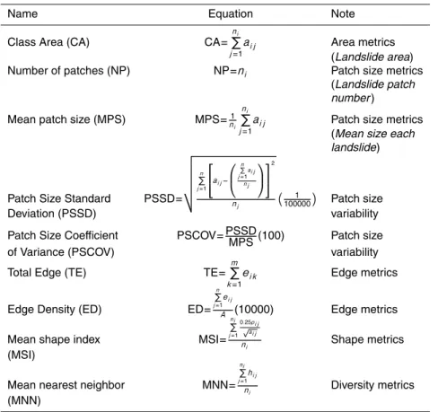
Table 1.Landscape metrics list.

Name Equation Note

Class Area (CA) CA=

ni P j=1

ai j Area metrics

(Landslide area)

Number of patches (NP) NP=ni Patch size metrics

(Landslide patch number)

Mean patch size (MPS) MPS=1

ni ni P j=1

ai j Patch size metrics

(Mean size each landslide)

Patch Size Standard PSSD=

v u u u u t n P j=1   ai j−

   n

P

j=1aij nj       2 nj 1 100000 Patch size

Deviation (PSSD) variability

Patch Size Coefficient PSCOV=PSSD_MPS(100) Patch size

of Variance (PSCOV) variability

Total Edge (TE) TE=

m P k=1

ei k Edge metrics

Edge Density (ED) ED=

n P j=1

ei j

A (10000) Edge metrics

Mean shape index MSI=

ni P j=1

0.25pij

√_aij

ni Shape metrics

(MSI)

Mean nearest neighbor MNN=

ni P j=1 hi j

n_i Diversity metrics

(MNN)

whereni is the number of patches in land-use classi;ai j is thejth patch area (ha) inland-use classi;mis the total

number of patch classes;ei k is the total length (m) of the edge between patch classesi andk;pi j is thejth patch

(20)

HESSD

7, 3423–3451, 2010

Y.-P. Lin et al.

Title Page

Tables Figures

◭ ◮

Back Close

Full Screen / Esc

Discussion

P

a

per

|

Dis

cussion

P

a

per

|

Discussion

P

a

per

|

Discussio

n

P

a

per

|

Table 2.Landslide history and major disturbances in study area.

Total (%) Landslide Mean size Disturbances and the information

landslide patch number each landslide Major Central Max. wind Max. 24-h

area (ha) (ha) Disturbances pressure (hPa) speed (m/s) rainfall (mm)

Image 1 1349.56 3.01 1728 0.78 Typhoon Herb 920.0 53.0 459

Image 2 684.44 1.52 827 0.83 Typhoon Zeb 920.0 55.0 326

Image 3 1572.20 3.50 1425 1.10 Chi-Chi Earthquake

Image 4 981.16 2.18 907 1.08 Typhoon Xangsane 960.0 38.0 550

Image 5 1445.28 3.22 1971 0.73 Typhoon Toraji 962.0 38.0 616

Image 6 1091.80 2.43 1580 0.69 Typhoon Dujuan 950.0 43.0 441

Image 7 812.12 1.81 1226 0.66 Typhoon Mindulle 942.0 45.0 288

Image 8 1313.68 2.93 2075 0.63 Typhoon Matsa 955.0 40.0 350

(%):percentage of total area

(21)

HESSD

7, 3423–3451, 2010

Y.-P. Lin et al.

Title Page

Tables Figures

◭ ◮

Back Close

Full Screen / Esc

Discussion

P

a

per

|

Dis

cussion

P

a

per

|

Discussion

P

a

per

|

Discussio

n

P

a

per

|

Table 3.Landscape metrics of spatial patterns with various landslide frequencies.

CA NP MPS PSSD PSCOV TE ED MSI MNN

(ha) (%) (ha) (ha) (m) (m) (m)

Pattern 1 1866.00 4.16 7020 0.27 0.50 187.96 1 875 760 1005.23 1.32 43.80

Pattern 2 792.00 1.76 4782 0.17 0.33 199.44 955 480 1206.41 1.25 48.77

Pattern 3 457.12 1.02 3196 0.14 0.23 159.15 591 760 1294.54 1.24 53.13

Pattern 4 296.68 0.66 2253 0.13 0.33 249.36 387 960 1307.67 1.21 61.90

Pattern 5 192.48 0.43 1391 0.14 0.20 147.89 254 800 1323.77 1.24 72.09

Pattern 6 152.24 0.34 823 0.18 0.34 182.46 169 080 1110.61 1.25 94.52

Pattern 7 101.12 0.23 440 0.23 0.64 276.96 106 400 1052.22 1.29 139.65

Pattern 8 81.28 0.18 131 0.62 1.81 291.77 48 000 590.55 1.31 372.27

(%):percentage of total area

(22)

HESSD

7, 3423–3451, 2010

Y.-P. Lin et al.

Title Page

Tables Figures

◭ ◮

Back Close

Full Screen / Esc

Discussion

P

a

per

|

Dis

cussion

P

a

per

|

Discussion

P

a

per

|

Discussio

n

P

a

per

|

Table 4. Logistic regression models with entire, low-occurrence and high-occurrence

land-slides.

Entire landslides Low-occurrence landslides High-occurrence landslides

Variable Coefficient P-value Coefficient P-value Coefficient P-value

Lithology <.001 <.001 .001

Metamorphic

Alluvim 0.45 <.001 0.55 <.001 ₋0.68 <.001

Hoshe 0.50 <.001 0.54 <.001 # #

Nanchuang 0.57 <.001 0.62 <.001 −0.14 .224

Wetness index 7.61E−02 <.001 7.41E−02 <.001 0.13 <.001

NDVI ₋28.42 <.001 ₋21.94 <.001 ₋39.40 <.001

Elevation −1.53E−03 <.001 −1.37E−03 <.001 −1.66E−03 <.001

Slope 2.94E−02 <.001 2.54E−02 <.001 3.30E−02 <.001

Distance to fault 1.40E−04 <.001 1.12E−04 <.001 1.41E−04 <.001

Distance to river 1.31E₋04 <.001 1.30E₋04 <.001 1.25E₋04 .005

Distance to road 1.60E₋04 <.001 1.75E₋04 <.001 5.10E₋05 .221

Distance to built-up land 1.83E−04 <.001 9.61E−05 <.001 4.31E−04 <.001

Const. 6.61 <.001 4.43 <.001 6.77 <.001

(23)

HESSD

7, 3423–3451, 2010

Y.-P. Lin et al.

Title Page

Tables Figures

◭ ◮

Back Close

Full Screen / Esc

Discussion

P

a

per

|

Dis

cussion

P

a

per

|

Discussion

P

a

per

|

Discussio

n

P

a

per

|

(24)

HESSD

7, 3423–3451, 2010

Y.-P. Lin et al.

Title Page

Tables Figures

◭ ◮

Back Close

Full Screen / Esc

Discussion

P

a

per

|

Dis

cussion

P

a

per

|

Discussion

P

a

per

|

Discussio

n

P

a

per

|

Fig. 2. Driving factors in logistic regression model(a)wetness index,(b)NDVI,(c)elevation,

(25)

HESSD

7, 3423–3451, 2010

Y.-P. Lin et al.

Title Page

Tables Figures

◭ ◮

Back Close

Full Screen / Esc

Discussion

P

a

per

|

Dis

cussion

P

a

per

|

Discussion

P

a

per

|

Discussio

n

P

a

per

|

(26)

HESSD

7, 3423–3451, 2010

Y.-P. Lin et al.

Title Page

Tables Figures

◭ ◮

Back Close

Full Screen / Esc

Discussion

P

a

per

|

Dis

cussion

P

a

per

|

Discussion

P

a

per

|

Discussio

n

P

a

per

|

(a) (b)

(c) (d)

Fig. 3. Landslide patterns after major disturbances on (a)8 November 1996,(b)31 October

(27)

HESSD

7, 3423–3451, 2010

Y.-P. Lin et al.

Title Page

Tables Figures

◭ ◮

Back Close

Full Screen / Esc

Discussion

P

a

per

|

Dis

cussion

P

a

per

|

Discussion

P

a

per

|

Discussio

n

P

a

per

|

(28)

HESSD

7, 3423–3451, 2010

Y.-P. Lin et al.

Title Page

Tables Figures

◭ ◮

Back Close

Full Screen / Esc

Discussion

P

a

per

|

Dis

cussion

P

a

per

|

Discussion

P

a

per

|

Discussio

n

P

a

per

|

0

500 1000

1500

2000

1

2

3

4

5

6

7

8 Occurrence number

CA (

h

a

)

0.0

0.2

0.4

0.6

0.8 MP

S

(

h

a

)

CA

MPS

Fig. 5. Landslide class area (CA) and mean patch size (MPS) of landslide with various

(29)

HESSD

7, 3423–3451, 2010

Y.-P. Lin et al.

Title Page

Tables Figures

◭ ◮

Back Close

Full Screen / Esc

Discussion

P

a

per

|

Dis

cussion

P

a

per

|

Discussion

P

a

per

|

Discussio

n

P

a

per

|

Fig. 6.Landslide susceptibility map with(a)entire landslides(b)low-occurrence landslides(c)