www.nat-hazards-earth-syst-sci.net/10/1307/2010/ doi:10.5194/nhess-10-1307-2010
© Author(s) 2010. CC Attribution 3.0 License.
and Earth
System Sciences
Assessment of earthquake-triggered landslide susceptibility in
El Salvador based on an Artificial Neural Network model
M. J. Garc´ıa-Rodr´ıguez1and J. A. Malpica2
1Universidad Polit´ecnica de Madrid, Escuela T´ecnica Superior de Ingenieros en Topograf´ıa, Geodesia y Cartograf´ıa
(ETSITGC), Departamento de Ingenier´ıa Topogr´afica y Cartograf´ıa, Madrid, Spain
2Universidad de Alcal´a, Escuela Polit´ecnica, Departamento de Matem´aticas, Madrid, Spain
Received: 6 November 2008 – Revised: 15 April 2010 – Accepted: 11 June 2010 – Published: 25 June 2010
Abstract. This paper presents an approach for assessing earthquake-triggered landslide susceptibility using artificial neural networks (ANNs). The computational method used for the training process is a back-propagation learning algo-rithm. It is applied to El Salvador, one of the most seismi-cally active regions in Central America, where the last se-vere destructive earthquakes occurred on 13 January 2001 (Mw7.7) and 13 February 2001 (Mw6.6). The first one
trig-gered more than 600 landslides (including the most tragic, Las Colinas landslide) and killed at least 844 people.
The ANN is designed and programmed to develop land-slide susceptibility analysis techniques at a regional scale. This approach uses an inventory of landslides and differ-ent parameters of slope instability: slope gradidiffer-ent, eleva-tion, aspect, mean annual precipitaeleva-tion, lithology, land use, and terrain roughness. The information obtained from ANN is then used by a Geographic Information System (GIS) to map the landslide susceptibility. In a previous work, a Lo-gistic Regression (LR) was analysed with the same param-eters considered in the ANN as independent variables and the occurrence or non-occurrence of landslides as dependent variables. As a result, the logistic approach determined the importance of terrain roughness and soil type as key factors within the model. The results of the landslide susceptibility analysis with ANN are checked using landslide location data. These results show a high concordance between the landslide inventory and the high susceptibility estimated zone. Fi-nally, a comparative analysis of the ANN and LR models are made. The advantages and disadvantages of both approaches are discussed using Receiver Operating Characteristic (ROC) curves.
Correspondence to:
M. J. Garc´ıa-Rodr´ıguez ([email protected])
1 Introduction
Landslide susceptibility studies are appropriate for evalua-tion and mitigaevalua-tion plans in potential landslide areas. There are several techniques available for landslide susceptibility research; however, due to uncertainty as an inherent nature of landslide phenomena, statistical and artificial intelligence approaches provide computational models to assess land-slide susceptibility over large regions. In January and Febru-ary 2001, El Salvador experienced several destructive earth-quakes that caused hundreds of landslides of various sizes. In this study, we have used an ANN model to assess the sus-ceptibility of the whole country of El Salvador to earthquake-induced landslides.
The first of those earthquakes occurred on 13 January 2001, with the epicentre located off the western coast of El Salvador in the subduction zone between the Cocos and Caribbean plates (Fig. 1). The earthquake had a magnitude ofMw7.7 and it produced more than 600 landslides, the most
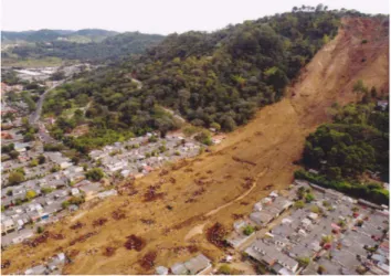
significant of them taking place in Santa Tecla, Las Colinas (Fig. 2), where 585 people died.
The second destructive earthquake occurred one month later, on 13 February, with a magnitude ofMw6.6. The
epi-centre was located to the west of San Miguel, this earthquake was associated with local faults that cross the country from east to west.
Fig. 1. DEM data together with the main epicentres of 2001 in El Salvador, tectonic features and landslide locations of 13 January 2001 earthquake (from ESRI shaded relief imagery which was developed using GTOPO30, Shuttle Radar Topography Mission (SRTM), and National Elevation Data (NED) data from the USGS).
Fig. 2.Earthquake-triggered landslide in Las Colinas, Santa Tecla (El Salvador, 13 January 2001), where 585 people died. The epicen-ter was located off the wesepicen-tern coast of El Salvador in the subduc-tion zone between the Cocos and Caribbean plates with a magnitude ofMw7.7 and a focal depth of 40 km (Benito et al., 2004).
2 Brief state of the art
Predicting future landslide locations requires a quantitative methodology to model these complex phenomena from past events with data gathered in the field or by other techniques, such as remote sensing, aerial photography or LIDAR. In the last few years, the development and the spread of soft com-puting applied to model natural phenomena have increased
exponentially. The fuzzy set theory, ANN, and genetic al-gorithms were applied to classification problems with the Geographic Information System (GIS), mainly because of their high capacity for analyzing heterogeneous and uncer-tain data.
Yesilnacar and Topal (2005) applied logistic regression (LR) analysis and neural networks to prepare a landslide suscep-tibility map for the rerouting of a pipeline after a segment of natural gas pipeline was damaged due to a landslide in Turkey. The strengths and weaknesses of these techniques were compared and the results found by ANNs were more realistic than those found by LR.
3 Application to El Salvador: data sources and GIS
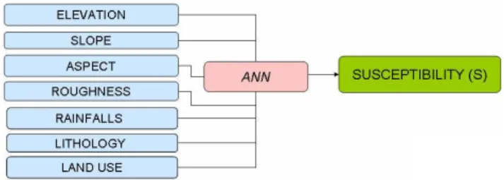
The methodology for the assessment of earthquake-triggered landslide susceptibility has involved the integration of data sources into a GIS (Fig. 3). The evaluation of suscepti-bility requires data input from variables representing phys-ical parameters known to contribute to the initiation of land-slides. El Salvador GIS is composed of diverse informa-tion including a 1:100 000 geological map, a 1:25 000 Dig-ital Cartography, precipitation data, ground strong motions records, epicentres catalogue, and an inventory of landslides. The landslides inventory used consists of data on slope move-ment from the 2001 El Salvador earthquakes compiled by the SNET (Servicio Nacional de Estudios Territoriales) of El Salvador. Descriptions and classifications of landslides were mainly based on the system developed by Cruden and Varnes (1996), which takes into consideration the type of movement, materials involved, and the state or activity of the unstable slopes. For our study, the inventory was processed and the debris flows were taken into account and separated from other types of mass movements, such as rock falls. Out of 235 samples, 112 belonged to this inventory as landslides and 123 samples were removed as non-landslides.
All of these layers of information from different sources and formats have been integrated into a GIS. In addition, there are other layers of generated maps and requirements, including Digital Terrain Model (DTM), slope map, aspect, roughness, and precipitation, for the assessment susceptibil-ity (Garc´ıa-Rodr´ıguez et al., 2008, 2009).
The physical properties of slope-forming materials, such as strength and permeability, are related to the lithology fac-tor, which therefore should affect the likelihood of slope fail-ure (Dai et al., 2002). The GIS information of lithology is structured into three types of layers: polygons (geologic, pe-dogenic, and volcanic classes), lines (faults, escarpments, dikes, paleo-riverbeds, and mineral seams), and points (fu-maroles, fossils, and volcanic classes). The surface geologic maps (scale 1:100 000) were digitised and georeferenced to obtain these data. The lithological units shown in the sur-face geologic maps were reclassified according to the clas-sification by the SNET and a generalized geologic map was produced in four types of rock and soil: hard rock, soft rock, consolidated soil, and unconsolidated soil (Garc´ıa-Rodr´ıguez et al., 2008). There are two lithological categories with rel-atively high landslide density: hard rock (43.2%) including pyroclastic deposits and associated volcaniclastics and
un-Fig. 3.GIS methodology for the assessment of earthquake-triggered landslide susceptibility.
consolidated soil (41.5%) including Tierra Blanca (TB) and Tobas de Color Caf´e (TCC). Generally, rock falls are initi-ated by tension in the upper half of the slopes, since TB and TCC are located in the upper part of the mountains.
A digital terrain model (DTM) can be used to classify the local relief and locate points of maximum and minimum heights. A model with a 100-m cell size was created from 20-m contour lines on the 1:25 000 topographic maps. The cell size was chosen for its suitability for work at a regional scale. Some terrain attributes, such as slope gradient and as-pect, were derived from the DTM. Slope gradient was calcu-lated using a 3×3 moving window based on of Horn’s (1981) algorithm. For slopes of uniform isotropic material, an in-creased slope gradient correlates with an inin-creased likelihood of failure. However, the soil thickness and strength may vary over a wide range among sites. Aspect can be defined as the slope direction, which identifies the downslope direction of the maximum rate of elevation change. The aspect of a slope can influence landslide initiation because it affects moisture retention and vegetation cover, which in turn affect soil strength and susceptibility to landslides. The amount of rainfall on a slope may also vary depending on its aspect (Wieczorek et al., 1997).
For the rainfall factor, we created a mean annual precipi-tation map with a resolution of 100×100 m. This was done through Kriging interpolation (Isaaks and Srivastava, 1989) from the precipitation database compiled by the SNET for the period 1961–1990.
In addition, the role of vegetation in slope stability is con-siderable. Some types of land use/cover, especially woody vegetation with large and strong root systems, provide both hydrological and mechanical effects that generally stabilize slopes (Montgomery et al., 2000). In contrast, more land-slides may be initiated in unvegetated areas. Therefore, land use/cover map from SNET was reclassified in 13 classes: ur-ban areas, forests, annual, mixed and permanent crops, mois-ture areas, swamps, mining, grasses, bush vegetation, indus-trial areas, artificial green, areas and lakes (Garc´ıa-Rodr´ıguez et al., 2008).
4 Artificial Neural Networks model
ANNs are generic non-linear function approximators that were developed by McCulloch and Pitts (1943) and exten-sively used for pattern recognition and classification. ANNs are networks of highly interconnected neural computing el-ements that have the ability to respond to input stimuli and to learn to adapt to the environment. ANN establishes rules during the learning phase and uses these rules to predict out-puts. The input neurons in the neural network are intrinsic factors to the slope instability, such as topographic, climatic, geological, and geotechnical data from different sources, and are stored in a GIS.
In order to cope with non-linear separable problems, such as the landslide phenomena, a complex model is needed. ANNs have shown their effectiveness dealing with non-linearity on several occasions (Ercanoglu et al., 2005). Be-cause ANNs have the ability to handle imprecise and fuzzy data, they can be used to work with continuous, categorical, and binary data without violating any assumptions. These techniques have been successfully applied to many prob-lems, including forecasting and prediction problems (Bishop, 1996). The ANN model is employed to analyze specific ele-ments related to the study area that contributed to landsliding in the past. The resulting information can then be used in the prediction of areas that may face landsliding in the future. The ANNs are programmed with error correction learning, which means that some desired response for the system must be known (Werbos, 1974; Parker, 1985).
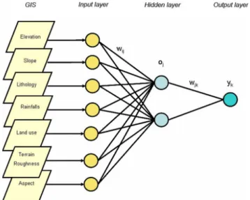
The behaviour of an ANN depends on the architecture of the network and on both the weights assigned to the connec-tions and the transfer function (Fig. 4). In our case, we have chosen seven input layers, one hidden layer, and one output layer. First, we present the system with the input data and obtain the output. Second, we adjust the system to make the output closer to what it should be. The first stage is referred to as feed-forward, and the second as back-propagation.
Fig. 4. Artificial Neural Network Architecture with seven neurons in the input layer to correspond to the independent variables. The
wijandwj krepresent the weights,ojrepresents values for the hid-den layer, andykrepresents the dependent variable, which gives of the current pixel’s degree of susceptibility for a landslide.
Fig. 5.A back-propagation neural network with the sigmoid func-tion used as activafunc-tion funcfunc-tion of the ANN.
4.1 Back-propagation algorithm
The back-propagation algorithm was applied to calculate the weights between the input layer and the hidden layer, and be-tween the hidden layer and the output layer. This was accom-plished by modifying the number of hidden nodes, the learn-ing rate and the momentum parameters until the aim was reached (minimum RMS values). The nodes perform non-linear input-output transformations by means of sigmoid ac-tivation functions. This structure of nodes and connections, known as the network topology, together with the weights of the connections, determines the final behaviour of the net-work.
pre-ceding layer. The expression is explicated by the equationhj (Eq. 1)
hj= X
i
wijxi (1)
wherewij is the weight between the nodeiand the nodej, andx is the output value from nodei. The value produced by the hidden nodej is the activation functionf evaluated at the sum produced within the nodej (Eq. 2):
oj=f hj=f n X
i wijxi
!
. (2)
oj is the output value from node j of the hidden layer. In turn, the output value is a function of the weight between the hidden and output layers, and the outputs of the input nodes (Eq. 3):
yk=f h X
i wj koj
!
. (3)
Wherey is the final response variable of the ANN. The acti-vation functionf is normally a non-linear sigmoid function, which is applied to the sumf of the weight of the inputs before proceeding to the next layer. It is used the sigmoid function (Eq. 4):
oj=f hj= 1
1+e−hj, (4)
which is easy to calculate because of its peculiar characteris-tic that its derivative is expressed with the same function, as shown in (Eq. 5),
f′ h
j=f hj 1−f hj. (5)
When developing a neural network for a particular problem, the data set is usually separated into two subsets: training and validation data. In the training set, the selection of sam-ples indicates the most relevant aspects for solving the prob-lem, while the validation data are useful for the evaluation of the neural network. The network architecture can be modi-fied, such as changing the number nodes in the hidden layer, learning rate and momentum parameter. The combination selected was [1, 0.9, 0.1], respectively. From the initial data, 80% was chosen randomly for training and the remaining 20% was used for validation. Initially, the network is pro-vided with random connection weights which represents the input to the network and the expected output. The weights are automatically modified to reduce the output error through an iterative procedure of back-propagation of errors. Conse-quently, the process is repeated until the tests are satisfactory. Using an ANN as a linear classifier would mean the use zero hidden layers. In our study, we have used one hidden layer, and tried several neurons within that layer. The more lay-ers and the more neurons within each layer that are used, the more non-linearity that is obtained. Theoretically, the more
non-linearity there is, the better the model would be for a natural phenomenon; however, more training samples would be needed to estimate the weights. We have observed that a large number of weights lead to poor generalizations, be-cause we have a limited number of training samples. The training rate is the other parameter of the ANN that we tuned although the convergence of the network was not very sen-sitive to it. Finally, 1000 iterations were taken for each test. While better results were seen with the higher the number of iterations, we observed that for most of the trials, stabiliza-tion happened around 200 iterastabiliza-tions.
4.2 Validation process
The total error of the model is defined by the formula (Eq. 6): ET=
X
k
E (6)
This error is a measure of the discrepancy between the net-works output value and the target (desired output) value. Neural network training is performed by trying to minimize the total error for the training set, as a function of the weights. The error is back-propagated through the neural network un-til the system minimized the sum of errorsETby changing
the weights between the layers. The adjusted weights can be expressed by the generalized delta equation (Eq. 7):
w′ij=wij+1wij (7)
where1wij is the incremental difference of weight, andηis the learning rate parameter, positive and less than one (Eq. 8):
1wij= −η ∂E ∂wij
(8)
The landslide susceptibility model must measure the accu-racy of the results in order to know the scientific significance (Chung and Fabbri, 1999, 2003). The validation of the anal-ysis was carried out by comparing the training sites and the estimated landslide map obtained by applying the weights derived from the ANN model.
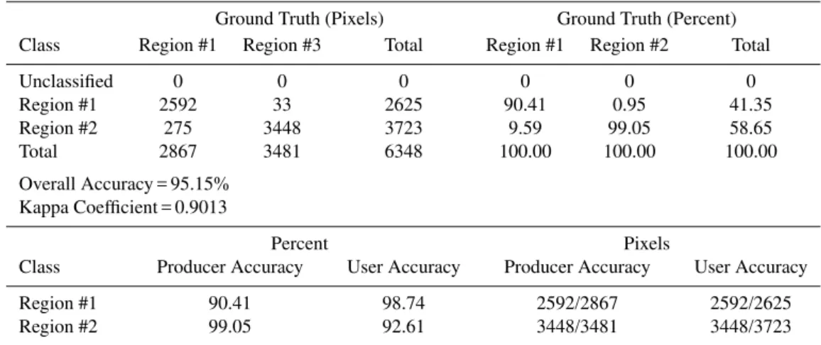
Table 1. Confusion matrix representing the number of pixels and percentage of ground truth for two regions: landslide (region #1) and non-landslide (region #2) and producer and user accuracy in number of pixels and percentage.
Ground Truth (Pixels) Ground Truth (Percent) Class Region #1 Region #3 Total Region #1 Region #2 Total
Unclassified 0 0 0 0 0 0
Region #1 2592 33 2625 90.41 0.95 41.35
Region #2 275 3448 3723 9.59 99.05 58.65
Total 2867 3481 6348 100.00 100.00 100.00
Overall Accuracy = 95.15% Kappa Coefficient = 0.9013
Percent Pixels
Class Producer Accuracy User Accuracy Producer Accuracy User Accuracy
Region #1 90.41 98.74 2592/2867 2592/2625
Region #2 99.05 92.61 3448/3481 3448/3723
The Kappa coefficient (k) is another measure of the clas-sification accuracy. It is calculated by the equation (Eq. 9):
k= NP
k
xkk−P k
xk6x6k
N2−P k
xk6x6k
(9)
whereN is the total number of pixels in all the ground truth classes, xkk is the element of the confusion matrix diago-nals, andxk6x6k is the elements of the ground truth pixels in a class times the sum of the classified pixels in that class summed over all classes.
The producer accuracy (PA) and user accuracy (UA) are shown in Table 1. The PA is a measure indicating the prob-ability that the classifier has labelled an image pixel into Class A, given that the ground truth is Class A. In the con-fusion matrix example, the region #1 class (landslide) has 2867 ground truth pixels, where 2592 pixels are classified correctly. The producer accuracy is the ratio 2592/2867, or 90.41%. UA is a measure indicating the probability that a pixel is Class A, given that the classifier has labelled the pixel into Class A. The classifier has labelled 2625 pixels as the region #1 class, and 2592 pixels are classified correctly. The user accuracy is the ratio 2592/2625 or 98.74%.
The ROC visualizes a classifier’s performance in order to select the proper decision threshold. It provides a proba-bility of detection versus a probaproba-bility of false alarm curve (Fawcett, 2006). ROCs are equivalent to prediction and success-rate curves proposed by Chung and Fabbri (2003). As can be observed from the ROC analysis (Fig. 6), the LR approach has a better performance than the ANN for a small range (between 0.0 and 0.07) of false alarms; however, when false alarms increase the ANN approach works better than LR. When false alarms are about 0.4, both techniques work similarly.
Fig. 6. The ROC curve calculated for the ANN model. The red color represents the LR model and blue color represents the ANN.
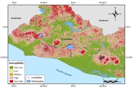
Fig. 7.Susceptibility map calculated from a methodology based on the ANN model.
Table 2. Number of pixels and percentage of susceptibility map classified into five levels: very low, low, medium, high, and very high.
Susceptibility Level
Very Low Low Medium High Very High N. pixels 954.799 68.723 71.186 707.064 267.731 Percentage (%) 46.1% 3.3% 3.4% 34.1% 12.9%
it cannot be said that LR is better than ANN is. What is in-teresting in the plot is the shape of the curves and how the curves cross, which we will discuss further in Sect. 6.
5 Susceptibility map
The main assumption in slope instability modelling is that the past occurrence of landslides at a specific site is indica-tive of the potential for future landslides to occur in sites with similar characteristics. The evaluation of susceptibility re-quires data input of variables representing physical parame-ters known to contribute to the initiation of landslides. An ANN model was estimated by incorporating the physical pa-rameters contributing to the formation of landslides. The ter-rain conditions of El Salvador were fed into the ANN model to calculate the landslide susceptibility. The susceptibility values obtained by this model were converted to a raster file in a GIS-based regional susceptibility, and a landslide susceptibility map for El Salvador was produced (Garc´ıa-Rodr´ıguez, 2009).
The results are shown in aSusceptibility Map (S)(Fig. 7), which defines the slope stability of an area into categories that range from stable to unstable. The susceptibility map in Fig. 7 is a representation of the histogram of the probabil-ity maps with different categories (Ayalew and Yamagishi, 2005). For our study, five susceptibility classes are chosen: very low, low, medium, high, and very high (Table 2). The classification of susceptibility is checked by the examination of the number of landslides locations within each class, the high and very high classes have 83% of landslides which sup-plies robustness to the ANN approach. For its representation, we used a color scheme that relates warm colors (red, orange, and yellow) to unstable and marginally unstable areas and cool colors (green shades) to stable areas. Similar to other studies, the landslide susceptibility model using ANN (Rossi et al., 2010) has a strong dichotomy in zonations, with a lim-ited number of intermediate susceptibilities (0.2–0.9).
6 Discussion and conclusions
Recently, we have worked with LR techniques using the same input data, and the results illustrated the importance of terrain roughness and soil type as key factors within the model; using only these two variables, the analysis returned a significance level of 89.4% (Garc´ıa-Rodr´ıguez et al., 2008, 2009). In the LR, the probability was estimated according to the logistic formula, which provided a deterministic model for the data and yielded weighted factors for each contribut-ing factor. It also allowed the calculation of the odds ratio, which represents the degree of risk associated with each fac-tor. However, LR fits the data to a fixed function, so it is less flexible and less capable of solving complex problems com-pared to ANNs. The advantages of ANNs and its possible application to the evaluation of landslide susceptibility come from the remarkable information processing characteristics of the artificial simulated biological system, including the ability to handle imprecise and fuzzy information, fault and failure tolerance, high parallelism, non-linearity, robustness, capability to generalize, and tolerance to noise data (Basheer and Hajmeer, 2000). On the other hand, a disadvantage is that they are known as black-box methods, since it is not known exactly how ANNs learn particular problems and ap-ply the extracted rules to new cases, or how conclusions can be drawn from the trained networks (G´omez and Kavzoglu, 2005). Although the accuracy produced in our work is of 95.1% for the ANN versus 89.4% for the LR, the black-box characteristic of the former does not allow for the investiga-tion of which variables are more influential to the response variable. However, this is possible with the LR because the weight of each factor is known.
Given that both the ANN and LR methods have great AU-ROC, only the ROC curves provides some subtle differences in the modus operandi of each classifier. For fewer false alarms, the sensibility of LR is superior to ANN, while for higher false alarm the superiority is for the ANN until a value of approximately of 0.4 of false alarms, when both classifiers perform similarly. This characteristic translates into Fig. 6, where it can be observed how the ANN gives broader areas of susceptibility than its correspondent for LR, as developed by Garc´ıa-Rodr´ıguez et al. (2008). The LR shows a more clearly defined area of susceptibility that corresponds to a steep ROC curve, while ANN gives a spread-defined area of susceptibility that corresponds to a gradual rise of the ROC curve.
ANNs have been used in areas which were once reserved for multivariate statistical analysis. Owing to this they are often considered to be statistical methods; however, it is nec-essary to be aware of subtle conceptual differences between these two methods in order to use ANNs effectively. In par-ticular, we are using a specific type of ANN called backprop-agation with one hidden layer, this is closely related to the statistic method called projection pursuit regression, which projects the data matrix of explanatory variables in the opti-mal direction. Compared with the statistical methods, neural networks allow the target classes to be defined with more
consideration to their distribution in the corresponding do-main of each data source (Zhou, 1999). The use of a GIS where the information is stored in layers facilitates imple-mentation of statistical or computational models, such as we have showed in this paper.
A literature review of recent works reveals that authors found ANN to be superior to other methods; particularly, some works compared LR and ANN using different variables and data; most of them confirm the superiority of ANN over LR. The first to compare these two methods were Yelsilnacar and Topal (2005); we have mentioned it above, they found ANN to be more realistic for landslide susceptibility map-ping. More recently, other authors also worked with LR and ANN for landslide susceptibility maps. Falaschi et al. (2009) compared LR and ANN and found ANN to be superior to LR. Yilmaz (2009) found ANN superior to frequency ratio and logistic regression; they both used ROC as the evalua-tion element. Pradhan and Lee (2010) also found ANN to be superior to frequency ratio and logistic regression for data for the Klang Valley, Malaysia; they performed trials with several different factors; in all cases, ANN was superior to LR.
Given the idiosyncrasy of the specific problem dealt with in this paper, such as scale and inventory, the ANN model is superior to the LR model in general terms, even though the AUROC is slightly better for the LR model, but there are others characteristics that should be taken into account when performing the analysis, such as flexibility of model, explicability of variables, and ROC shape. Finally, it could be said that there is no a best model for all cases, it depends on many factors including the number of training samples, the independent variables being considered, and the scale.
Acknowledgements. This research has been developed within
the framework of the ANDROS Project, and was financed by the Spanish Ministry of Science and Education (CGL2005-07456-C03-03/BTE), the Ministry of Science and Innovation (CGL2009-13768) and Technical University of Madrid - Latin-American Relationships (AL08-PID-038). Cartography data have been provided by the Ministerio de Ambiente y Recursos Naturales (MARN) of the El Salvador. The authors thank these contributors, and especially to Bel´en Benito, for their support. The authors would also like to express their gratitude to Editor A. G¨unther, reviewer H.-B. Havenith and two anonymous reviewers, for their constructive criticisms of an earlier version of this paper.
Edited by: A. G¨unther
Reviewed by: H.-B. Havenith and two anonymous referees
References
Band, L. E.: Spatial aggregation of complex terrain, Geogr. Anal., 21, 279–293, 1989.
Basheer, I. A. and Hajmeer, M.: Artificial neural networks: funda-mentals, computing, design and application, J. Microbiol. Meth., 43, 3–31, 2000.
Benito, B., Cepeda, J. M., and Mart´ınez D´ıaz, J. J.: Analysis of the spatial and temporal distribution of the 2001 earthquakes in El Salvador, in: Geological Society of America Special Paper 375, Natural Hazards in El Salvador, edited by: Rose, W. I., Bom-mer, J. J., L´opez, D. L., Carr, M. J., and Major, J. J., Boulder, Colorado, 339–356, 2004.
Bishop, C. M.: Neural Networks for Pattern Recognition, 1st edn., Oxford University Press, USA, 1996.
Chung, C. F. and Fabbri, A .G.: Probabilistic prediction models for landslide hazard mapping, Photogramm. Eng. Rem. S., 65, 1389–1399, 1999.
Chung, C. F. and Fabbri, A. G.: Validation of spatial prediction models for landslide hazard mapping, Nat. Hazards, 30, 451– 472, 2003.
Cruden, D. M. and Varnes, D. J.: Landslides Types and Processes, in: Landslides: investigation and mitigation, Special Report 247, En Transportation Research Board, National Research Council, edited by: Turner, A. K. and Shuster, R. L., Washintong, DC, 36–71, 1996.
Dai, F. C. and Lee, C. F.: Landslide characteristics and slope insta-bility modeling using GIS, Lantau Island, Hong Kong, Geomor-phology, 42, 213–228, 2002.
Ercanoglu, M.: Landslide susceptibility assessment of SE Bartin (West Black Sea region, Turkey) by artificial neural networks, Nat. Hazards Earth Syst. Sci., 5, 979–992, doi:10.5194/nhess-5-979-2005, 2005.
Ermini, L., Catani, F., and Casagli, N.: Artificial neural networks applied to landslide susceptibility assessment, Geomorphology, 66, 327–343, 2005.
Falaschi, F., Giacomelli, F., Federici, P. R., Puccinelli, A., D’Amato Avanzi, G., Pochini, A., and Ribolini, A.: Logistic regression versus artificial neural networks: landslide susceptibility eval-uation in a sample area of the Serchio River valley, Italy, Nat. Hazards, 50, 551–569, 2009.
Fawcett, T.: An introduction to ROC analysis, Pattern Recogn. Lett., 27, 861–874, 2006.
Garc´ıa-Rodr´ıguez, M. J., Malpica, J. A., Benito, B., and D´ıaz, M.: Susceptibility assessment of earthquake-triggered landslides in El Salvador using logistic regression, Geomorphology, 95, 172– 191, 2008.
Garc´ıa-Rodr´ıguez, M. J.: Metodologias para la evaluaci´on de peligrosidad a los deslizamientos inducidos por terremotos, Ph.D. thesis, Universidad de Alcal´a, Espa˜na, 300 pp., 2009. G´omez, H. and Kavzoglu, T.: Assessment of shallow landslide
susceptibility using artificial neural networks in Jabonosa River Basin, Venezuela, Eng. Geol., 78, 11–27, 2005.
Horn, B. K. P.: Hill-shading and the reflectance map, in: Proceed-ings of the IEEE, 69, 14-47, 1981.
Hosmer, D. W. and Lemeshow, S.: Applied Logistic Regression, 2nd edn., Wiley, New York, 2000.
Isaaks, E. H. and Srivastava, R. M.: An Introduction to Applied Geostatistics, Oxford University Press, Oxford, 1989.
Lee, S., Ryu, J. H., Lee, M. J., and Won, J. S.: Use of an artificial neural network for analysis of the susceptibility to landslides at Boun, Korea, Environ. Geol., 44, 820–833, 2003a.
Lee, S., Ryu, J. H., Min, K., and Won, J. S.: Landslide susceptibility analysis using GIS and artificial neural network, Earth Surf. Proc. Land., 28, 1361–1376, 2003b.
Lee, S., Ryu, J. H., Won, J. S., and Park, H. J.: Determination and application of the weights for landslide susceptibility map-ping using an artificial neural network, Eng. Geol., 71, 289–302, 2004.
Lee, S.: Application of logistic regression model and its validation for landslide susceptibility mapping using GIS and remote sens-ing data, Int. J. Remote Sens., 26, 1477–1491, 2005.
McCulloch, W. S. and Pitts, W. H.: A logical calculus of the ideas immanent in nervous activity, B. Math. Biophys., 5, 115–133, 1943.
Mardia, K. V.: Statistics of directional data, Academic Press, Lon-don, 1972.
Montgomery, D. R., Schmidt, K. M., Greenberg, H. M., and Diet-rich, W. E.: Forest clearing and regional landsliding, Geology, 28, 311–314, 2000.
Parker, D. B.: Learning logic, Technical report TR-47, Center for Computational Research in Economics and management Sci-ence, MIT, Cambridge, MA, 1985.
Pradhan, B. and Lee, S.: Landslide susceptibility assessment and factor effect analysis: backpropagation artificial neural networks and their comparison with frequency ratio and bivariate logis-tic regression modelling, Environ. Modell. Softw., 25, 747–759, 2010.
Rossi, M., Guzzetti, F., Reichenbach, P., Mondini, A.. and Peruc-cacci, S.: Optimal landslide susceptibility zonation based on multiple forecasts, Geomorphology, 114, 129–142, 2010. Upton, G. J. G. and Fingleton, B.: Spatial Data Analysis by
Exam-ple, John Wiley & Sons, Chichester, 1989.
Werbos, P.: Beyond Regression: New Tools for Prediction and Analysis in the Behavioral Sciences, Ph.D. thesis, Harvard Cam-bridge, MA, 1974.
Wieczorek, G. F., Mandrone, G., and DeCola, L.: The influence of hillslope shape on debris-flowinitiation, in: Debrisflow Hazards Mitigation: Mechanics, Prediction, and Assessment American Society of Civil Engineers, edited by: Chen, C. L., New York, 21–31, 1997.
Yesilnacar, E. and Topal, T.: Landslide susceptibility mapping: a comparison of logistic regression and neural networks methods in a medium scale study, Hendek region (Turkey), Eng. Geol., 79, 251–266, 2005.
Yilmaz, I.: Landslide susceptibility mapping using frequency ratio, logistic regression, artificial neural networks and their compari-son: a case study from Kat landslides (Tokat-Turkey), Comput. Geosci., 35, 1125–1138, 2009.