An Original Stepwise Multilevel Logistic
Regression Analysis of Discriminatory
Accuracy: The Case of Neighbourhoods and
Health
Juan Merlo1*, Philippe Wagner1,2, Nermin Ghith1,3, George Leckie4
1Unit for Social Epidemiology, Faculty of Medicine, Lund University, Malmö, Sweden,2Centre for Clinical Research Västmanland, Uppsala University, Uppsala, Sweden,3Research Unit of Chronic Conditions, Bispebjerg University Hospital, Copenhagen, Denmark,4Centre for Multilevel Modelling, University of Bristol, Bristol, United Kingdom
Abstract
Background and Aim
Many multilevel logistic regression analyses of“neighbourhood and health”focus on inter-preting measures of associations (e.g., odds ratio, OR). In contrast, multilevel analysis of variance is rarely considered. We propose an original stepwise analytical approach that dis-tinguishes between“specific”(measures of association) and“general”(measures of vari-ance) contextual effects. Performing two empirical examples we illustrate the methodology, interpret the results and discuss the implications of this kind of analysis in public health.
Methods
We analyse 43,291 individuals residing in 218 neighbourhoods in the city of Malmö, Swe-den in 2006. We study two individual outcomes (psychotropic drug use and choice of private vs. public general practitioner, GP) for which the relative importance of neighbourhood as a source of individual variation differs substantially. In Step 1 of the analysis, we evaluate the OR and the area under the receiver operating characteristic (AUC) curve for individual-level covariates (i.e., age, sex and individual low income). In Step 2, we assess general contex-tual effects using the AUC. Finally, in Step 3 the OR for a specific neighbourhood character-istic (i.e., neighbourhood income) is interpreted jointly with the proportional change in variance (i.e., PCV) and the proportion of ORs in the opposite direction (POOR) statistics.
Results
For both outcomes, information on individual characteristics (Step 1) provide a low discrimi-natory accuracy (AUC = 0.616 for psychotropic drugs; = 0.600 for choosing a private GP). Accounting for neighbourhood of residence (Step 2) only improved the AUC for choosing a private GP (+0.295 units). High neighbourhood income (Step 3) was strongly associated to choosing a private GP (OR = 3.50) but the PCV was only 11% and the POOR 33%.
a11111
OPEN ACCESS
Citation:Merlo J, Wagner P, Ghith N, Leckie G (2016) An Original Stepwise Multilevel Logistic Regression Analysis of Discriminatory Accuracy: The Case of Neighbourhoods and Health. PLoS ONE 11 (4): e0153778. doi:10.1371/journal.pone.0153778
Editor:Mirjam Moerbeek, Utrecht University, NETHERLANDS
Received:August 17, 2015
Accepted:April 4, 2016
Published:April 27, 2016
Copyright:© 2016 Merlo et al. This is an open access article distributed under the terms of the
Creative Commons Attribution License, which permits unrestricted use, distribution, and reproduction in any medium, provided the original author and source are credited.
Data Availability Statement:All relevant data are within the paper and its Supporting Information files.
Funding:This work was supported by the Swedish Research Council (JM, 2013-2484)http://www.vr.se/ inenglish.4.12fff4451215cbd83e4800015152.html. The funders had no role in study design, data collection and analysis, decision to publish, or preparation of the manuscript.
Conclusion
Applying an innovative stepwise multilevel analysis, we observed that, in Malmö, the neigh-bourhood context per se had a negligible influence on individual use of psychotropic drugs, but appears to strongly condition individual choice of a private GP. However, the latter was only modestly explained by the socioeconomic circumstances of the neighbourhoods. Our analyses are based on real data and provide useful information for understanding neigh-bourhood level influences in general and on individual use of psychotropic drugs and choice of GP in particular. However, our primary aim is to illustrate how to perform and interpret a multilevel analysis of individual heterogeneity in social epidemiology and public health. Our study shows that neighbourhood“effects”are not properly quantified by reporting differ-ences between neighbourhood averages but rather by measuring the share of the individual heterogeneity that exists at the neighbourhood level.
Introduction
An established area of research in social epidemiology and public health concerns the
investiga-tion of“neighbourhood and health”and multilevel logistic regression analyses are frequently
conducted for this purpose [1,2] [3,4] [5] [6]. Interest within such studies typically lies in
esti-mating and interpreting measures of associations (e.g., the exponentiated regression coefficients or odds ratios, OR) between specific contextual characteristics and binary measures of individ-ual health outcomes. In other settings, researchers routinely perform analyses of small area
vari-ation which, in their simplest form, are displayed as health league tables,“heat”or choropleth
maps, or atlases of geographical variation. A common denominator in all these studies is that they analyse differences between group averages. For instance, the average risk of dying among individuals living in poor neighbourhoods might be compared to the average risk of dying among individuals living in rich neighbourhoods. Alternatively, statistics like indices of small area variation might be calculated to summarize the overall range or variation in group averages. All these studies disregard within-group individual-level variation in health outcomes except to estimate the statistical uncertainty around the estimated differences between group averages
In contrast, other researchers have explicitly concluded that we need to consider both differ-ences between group averages and differdiffer-ences between individuals around these averages. In fact, information on individual-level variance in multilevel regression analysis provides
indis-pensable information for understanding contextual influences on health [1–13] From this
per-spective, knowing the proportions of overall variation in health outcomes which are attributable to the contextual-level (e.g., the neighbourhood) is of fundamental relevance for
operationalizing contextual phenomena and for identifying the relevant levels of analysis [3,7,
11,14–18]. This concept is rather intuitive when we think about the analogy between
individ-ual and collective bodies [7]. Also, using Rose’s terminology [19], in order to identify sick
pop-ulations the simple quantification of differences between population averages of some health indicator is not appropriate. Rather, we need information on both population averages and the distribution of individual values around these averages. Through doing so, we are able to learn the share of the total outcome variance that is between population level averages so the larger
this proportion, the more relevant the population level of analysis is [11]. This idea
corre-sponds well with the notion of variance partition coefficients (VPC) and the concept of
Considering these ideas, we can identify at least three different analytical approaches in social epidemiology, all of which are dedicated to the investigation of contextual influences on binary measures of individual health.
Thesmall area variation approachfocuses on the analysis of geographic variance using
aggregated geographical data often on small areas or zones at different spatial scales [20].
Themultilevel analysis of associations approachperforms multilevel logistic regression anal-ysis or similar techniques to identify average associations (e.g., ORs) between specific
contex-tual level variables and individual health adjusting for neighbourhood clustering [21],.
Finally, themultilevel analysis of individual heterogeneity approachcombines both the
mul-tilevel analysis of associations for estimation of specific contextual effects and the mulmul-tilevel analysis of variance (e.g., the degree of clustering, ICC) for the investigation of general
contex-tual effects (i.e., non-specific contexcontex-tual influences on health) [7] [4].
Thesmall area variation approachtypically applied in Public Health represents a refinement
of classical ecological studies on aggregated data. Themultilevel analysis of associations
approachfollows the conventional approach in probabilistic risk factors epidemiology [22],
while themultilevel analysis of individual heterogeneity approachadopts a multilevel
perspec-tive for understanding heterogeneity of individual responses around the average risk in a group
[2]. It is this last approach which we develop and promote in this study.
Interestingly, in spite of their independent origins and areas of application, themultilevel
analysis of individual heterogeneity approachhas many analogies with that adopted in other fields of epidemiology concerned with the identification of new candidate risk factors and biomarkers and the evaluation of diagnostic and screening test. In those research fields, it is well known that measures of average association like ORs provide limited information for gauging the
perfor-mance of a diagnostic, prognostic, or screening marker [23]. Accordingly, the rule is that
mea-sures of association need be interpreted together with meamea-sures of discriminatory accuracy such,
the area under the receiver operating characteristic curve (AUC) [24,25]. Analogously, the
mul-tilevel analysis of individual heterogeneity approachargues that estimates of specific contextual effects (i.e., average measures of association) provide insufficient information if they are not
accompanied by measures of general contextual effects (i.e., degree of clustering) [2–4].
In themultilevel analysis of individual heterogeneity approachthe ICC for hierarchical
mul-tilevel structures [26] is a fundamental measure for quantifying general contextual effects. As a
concept, the ICC (i.e., the share of the total outcome variance which lies at the context level, having adjusted for any covariates) is rather intuitive for continuous responses since the indi-vidual- and contextual-level variances are both estimated and defined on the same scale. How-ever, the ICC proves less straightforward to understand and calculate when analysing binary responses via multilevel logistic regression because only the contextual-level variance is esti-mated. Furthermore, this variance is defined on the log-odds scale, rather than the binary
response scale [26]. Nevertheless, a range of procedures for calculating the ICC for binary
responses have been proposed, including a normal response approximation, the simulation
method, and the Taylor series linearization, [14,26–28]. However, it is the ICC based on the
latent response formulation of the model which has become most widely adopted. No doubt partly due to these complications, a range of alternatives to the ICC for binary responses have also been proposed to quantify the extent of general contextual effects. These include the
pair-wise odds ratio (PWOR)[18] and measures of heterogeneity such as the median odds ratio
(MOR)[29,30]. In any case, it is important to realize that the ICC is itself a measure of
discrim-inatory accuracy [31,32]. Therefore, taking advantage of the analogy between the concept of
discriminatory accuracy and the notion of general contextual effects, a simple but innovative approach is to express general contextual effects by means of measures of discriminatory
public health practitioners and physicians and its computation is straightforward using stan-dard statistical software.
In the current study, we present a novel three-step approach for the systematic investigation of observational multilevel (e.g., individual and neighbourhood) effects on binary measures of individual health and health care utilization, distinguishing between specific and general con-textual effects. To make our approach as accessible as possible, we present a conceptual and didactic treatment of the issues rather than a technical and mathematical one. We introduce and then demonstrate the utility of AUC as a measure of general contextual effects and we compare it to the ICC and the MOR. We illustrate our approach by analysing two different binary outcomes: (i) use of psychotropic medication, which is related to both psychological health and access to medication; and (ii) individual choice of a private vs. a public general prac-titioner (GP), which is a behavioural outcome.
Population and methods
Study sample
We drew our sample of individuals from the LOMAS (Longitudinal Multilevel Analysis in Sca-nia) database containing fully anonymised data on all individuals living in the county of Scania,
Sweden during the years 1968–2006. The database includes geographic, demographic and
socioeconomic information on all individuals as well as data on their health care and
medica-tion use [35]. The sample consists of all individuals aged 35–64 years residing in the city of
Malmö on 31st December 2005 (N = 99,266), who were still alive on 31st December 2006 (N = 98,536). We further restricted this sample to those with at least one contact with primary health care during the year 2006 (N = 46,675) as well as residing in neighbourhoods with at least 30 people who fulfilled the same selection criteria (N = 43,588). The reason for the latter was to further ensure the anonymity of the database. Otherwise, the size of the neighbourhood is not a problem for performing multilevel regression analysis as small neighbourhoods provide uncertain information and are shrunken towards the overall mean in the multilevel regression
[16]. Lastly, we dropped 297 (0.7%) individuals who had missing values for individual income.
The final study sample consisted of 43,291 individuals within 218 neighbourhoods. Our study is representative for those individuals with at least a one contact with primary health care and this condition is necessary to investigate the choice of a private versus a public GP. However, in the case of psychotropic drug use we could have studied the whole sample of
people 35–64 year old. Therefore, strictly our analysis concerns use of psychotropic drugs
among primary health care patients rather than the whole population.
The National Board of Health and Welfare and Statistics Sweden constructed the initial LOMAS database by means of record linkage of different registers using the unique Swedish personal identification number. Finally, the Swedish authorities delivered the LOMAS database to us without the personal identification numbers to ensure the anonymity of the subjects and after aprobal from The Regional Ethics Review Board in southern Sweden as well as the data safety committees from the National Board of Health and Welfare and from Statistics Sweden.
For the purpose of our study we used the LOMAS database to create a fully anonymized sample that besides the exclusion criteria contained only information on gender, age in 5-year groups, as well as individual and neighbourhood income in two categories. We also deleted and replaced the identification codes of the neigbourhoods and the LOMAS codes of the indi-viduals. This fully anonymized sample provides sufficient information to replicate our analyses but completely prevent the identification or specific individual or neighbourhoods. This
sam-ple is provided in the Online Supsam-plementary Materials in MLwiN format (S1 Data), SPSS
Assessment of variables
Outcome variables. To illustrate our three-step approach, we carried out two empirical analyses. In the first analysis the outcome variable was defined as use (= 1) or not (= 0) of psy-chotropic medication during 2006. We defined psypsy-chotropic medication as Anatomical
Thera-peutic Chemical (ATC) Classification System [36] codes N05B (Anxiolytics), N05C
(Hypnotics and sedatives) and N06A (Antidepressants). In the second analysis, the response variable was whether a person had visited a private (= 1) or public (= 0) specialist physician in a general practice (GP) during the year.
Individual characteristics
In order to illustrate our approach as clearly as possible, we considered only three
individual-level covariates: age categorized into six age groups, 35–39, 40–44, 45–49, 50–54, 55–59, and
60–64 years, using the youngest age group as the reference category in the model specifications;
sex that compared men (= 1) with women (= 0); and income categorized as‘low’when having
less that the median income in Malmö, or‘high’otherwise. In the analysis of psychotropic
medication the reference category was high income while in the analysis of private GP choice the reference category was low income. These choices are cosmetic, but ensure that we estimate positive rather than negative associations between the outcome and income which are easier for readers to interpret (psychotropic medication use is higher among the poor while private GP use is higher among the rich). The median income in Malmö was derived from individual-ized household disposable income in 2004 for all individuals aged 35 to 85 in the city.
Neighbourhood variables
We definedneighbourhoodsusing small-area market statistics (SAMS) boundaries created by
Statistics Sweden [37]. The SAMS boundaries are based on municipalities’sub-division
bound-aries which are constructed to maximise the internal homogeneity of housing tenure. The resulting neighbourhoods have an average population of around 1000 individuals.
For simplicity, we categorized neighbourhoods as‘rich’or‘poor’according to whether the
proportion of low income individuals in each neighbourhood was below the median across all neighbourhoods in the city. Paralleling the way we entered individual income into our models, in the analysis of psychotropic medication use we set the reference category for neighbourhood income to be rich neighbourhoods while in the analysis of private GP use we set the reference category to be poor neighbourhoods.
Multilevel analysis of heterogeneity
The data have a two-level hierarchical structure with individuals (level 1) nested within neigh-bourhoods (level 2). For the analysis we applied a three step-approach consisting of fitting, interpreting and contrasting the results of three consecutive two-level logistic regression mod-els: the individual effects model (Step 1); the general contextual effects model (Step 2); and the specific contextual effects model (Step 3).
Letyijdenote the binary response of interest (e.g., use of psychotropic medication or private
GP) for individuali(i= 1,. . .,nj) in neighbourhoodj(j= 1,. . .,J).
Step 1—The individual effects model. Step 1 simply consists of fitting a conventional
sin-gle-level logistic regression foryijincluding only the individual-level covariates;
information (S1andS4Models). The model is therefore written as
yij Binomialð1; pijÞ; ð1Þ
logitðpijÞ ¼b0þb1ageijþb2sexijþb3incomeij; ð2Þ
whereπijdenotes the probability that individualiin neighbourhoodjuses psychotropic
medi-cation (or private GP) given their individual characteristics ageij, sexijand incomeij.
The regression coefficientsβ1,β2,β3measure the associations between the log-odds of the
health outcome and each covariate all else equal and when exponentiated these are translated to ORs. For ease of illustration we have entered age into the model linearly, but we shall relax
this assumption when we fit the model. Post-estimation, predicted probabilities^p
ijare
calcu-lated for each individual and are used to calculate the AUC for the model.
The AUC [33,34] is constructed by plotting the true positive fraction (TPF) (i.e., sensitivity)
against the false positive fraction (FPF) (i.e., 1−specificity) for different binary classification
thresholds of the predicted probabilities. The AUC measures the ability of the model to cor-rectly classify individuals with or without the outcome (e.g., using or not psychotropic
medica-tion or visiting a private vs. a public GP) as a funcmedica-tion of individuals’predicted probabilities.
The AUC takes a value between 1 and 0.5 where 1 is perfect discrimination and 0.5 would be as
equally as informative as flipping a coin [23] (i.e., the covariates have no predictive power).
The AUC of the Step 1 model quantifies the accuracy of using individual-level information alone for identifying individuals with the outcome.
There are alternative measures of discriminatory accuracy like net reclassification
improve-ment (NRI) and the integrated discrimination improveimprove-ment (IDI) [38–40]. However, the NRI
and IDI depend on the calibration of the models and are non-proper evaluation metrics so the
use of these measures is not recommendable [41].
Step 2–The general contextual effects model. Step 2 consists of extending the Step 1
model from a conventional single-level logistic regression model to a two-level individuals-within-neighbourhoods logistic regression model. See also the MLwiN worksheets fitting this
model in supplementary information (S2andS5Models). This extended model is written as
yij Binomialð1;pijÞ; ð3Þ
logitðpijÞ ¼b0þb1ageijþb2sexijþb3incomeijþuj; ð4Þ
uj Nð0
;s
2
uÞ; ð5Þ
whereujdenotes the random effect for neighbourhoodj. These effects are assumed normally
distributed with zero mean and variances2
u, a parameter to be estimated.
Postestimation, values can be assigned to these effects via empirical Bayes prediction. These
predictionsu^
jare sometimes referred to as shrinkage estimates as their values are shrunk
towards the population-average of zero by a shrinkage factor proportional to the amount of information available on each neighbourhood (essentially the neighbourhood size). Shrinkage is desirable as it protects one against over interpreting the otherwise often extreme predictions associated with very small neighbourhoods. The statistical uncertainty surrounding these
pre-dictions can also be calculated and communicated via error bars (e.g., 95% confidence
inter-vals). This uncertainty must be taken into account when ranking neighbourhoods, for example by predicted prevalence of the health outcome, as such rankings have been shown to be
More generally, the interpretation of neighbourhood rankings needs be done in relation to the
general contextual effect(see elsewhere for empirical examples) [4].
Thegeneral contextual effectis appraised using the estimated between-neighbourhood
vari-ance^s2
uas this quantifies the variability in unobserved influences on the health outcome
com-mon to individuals living in in the same neighbourhood. Thus,s^2
uis assumed to reflect
variation in any direct effects of neighbourhood context captured by the neighbourhood
boundaries (i.e.,“causal”effect of place). However, in an observational study, it might also
reflect neighbourhood compositional differences in unmodelled individual characteristics (e.g.,
unobserved selection of individuals into neighbourhoods). We calculated three different
mea-sures ofgeneral contextual effects: (i) the change in the AUC compared with the Step 1 model;
(ii) the ICC; and (iii) the MOR.
1. While the AUC of the Step 1 model quantifies the accuracy of using individual-level infor-mation alone for identifying individuals with, or without the outcome, the predicted proba-bilities from the Step 2 model are based on both the individual-level covariates and the
predicted neighbourhood random effectu^j. Consequently, the AUC of the Step 2 model can
be compared with that from Step 1 to quantify the added value of having information on
the neighbourhood of one’s residence when it comes to identifying the outcome of the
indi-viduals. Therefore, in this approach the general contextual effect of the neighbourhood is appraised by quantifying the increase in the AUC achieved when adding general neighbour-hood information to the individual level predictions calculated in the Step 1 model. The larger this difference, the greater the general neighbourhood effect is.
2. We chose to calculate the ICC based on the latent response formulation of the model as it is the approach most widely adopted in applied work. This formulation assumes a latent con-tinuous response underlies the observed binary response and it is this latent response for which the ICC is calculated and interpreted. The higher the ICC, the more relevant
neigh-bourhood context is for understanding individual latent response variation [14,16,26]. The
ICC is calculated as
r¼ s
2 u
s2 uþ
p2 3
ð6Þ
wherep2
3 denotes the variance of a standard logistic distribution. (Note that hereπdenotes the
mathematical constant 3.1416. . ., not the probability.)
3. The MOR [14,29,30] is an alternative way of interpreting the magnitude of the
neighbour-hood variance. The MOR translates the neighbourneighbour-hood variance estimated on the log-odds scale, to the widely used OR scale. This makes the MOR comparable with the OR of individ-ual and neighbourhood covariates. The MOR is defined as the median value of the distribu-tion of ORs obtained when randomly picking two individuals with the same covariate values from two different neighbourhoods, and comparing the one from the higher risk neighbourhood to the one from the lower risk neighbourhood. In simple terms, the MOR can be interpreted as the median increased odds of reporting the outcome if an individual moves to another neighbourhood with higher risk. Therefore, the higher the MOR the greater the general contextual effect. The MOR is calculated as
MOR¼expð ffiffiffiffiffiffiffi
2s2
u
p
F 1
ð0:75ÞÞ; ð7Þ
whereF−1() represents the inverse cumulative standard normal distribution function. In
absence of neighbourhood variation (i.e.,s2
Step 3–The specific contextual effects model. Step 3 consists of adding the
neighbour-hood covariate of interest to the model in order to estimate the specific OR for a contextual var-iable. In our case we are interested in the effect of neighbourhood income (i.e., rich or poor) on each outcome. See also the MLwiN worksheet for fitting this model in supplementary
informa-tion (S3andS6Models). The step 3 model can be written as
yijBinomialð1;pijÞ; ð8Þ
logitðpijÞ ¼ b0þb1ageijþb2sexijþb3incomeijþb4nincomejþuj; ð9Þ
ujNð0;s
2
uÞ; ð10Þ
where nincome denotes the additional neighbourhood covariate.
Specific contextual effects measure the associations between contextual characteristics of the neighbourhood (e.g., rich or poor neighbourhood) and the individual outcome. As in the case of individual-level observational effects, specific contextual effects are estimated using mea-sures of average effect such as ORs. However, an extended misunderstanding when applying
multilevel regression analyses is to give a“population average”interpretation to the OR of
con-textual variables [14,29,30].
The point is that the multilevel regression provides regression coefficients for individual variables that are adjusted for the neighbourhood-level random effects. That is, they reflect the association between individual level variables and the outcome within a specific
neighbour-hood. They are therefore termed‘‘neighbourhood specific”or‘‘cluster specific”ORs. However,
in multilevel logistic regression, a contextual OR can hardly be interpreted in this way since the contextual variable is constant for all individuals in the neighbourhood. The contextual OR can at best be interpreted as contrasting two neighbourhoods differing in the value of the contex-tual variable by one-unit, but which have identical value for the neighbourhood-level random
effects (and all other covariates). To avoid this difficult interpretation, Larsenet al[29,30]
pro-posed the use of the 80% interval odds ratio (IOR-80%) as a way of including the neighborhood variance in the quantification of a contextual OR.
The lower and upper bounds of the IOR-80% for nincome are calculated as
expðb4
ffiffiffiffiffiffiffi
2s2
u
p
F 1
ð0
:9ÞÞ: ð11Þ
The IOR-80% is defined as the middle 80% range of the distribution of ORs formed by mak-ing random pairwise comparison between neighbourhoods exposed and non-exposed to the contextual variable. The IOR-80% interval is narrow if the between-neighbourhood variance s2
uis small, and it is wide if the between-neighbourhood variance is large. If the IOR-80%
inter-val contains 1, then for some neighbourhoods the association is in the opposite direction to the
overall OR [29] [14].
An alternative to the IOR-80% is the Proportion of Opposed Odds Ratios (POOR). That is,
the proportion of ORs with the opposite direction to the overall OR [14]. The values of the
POOR extend between 0% and 50%. A POOR of 0% means all ORs have the same sign. A POOR of 50% means that half of the ORs are of the opposite sign and so the association is very heterogeneous. For our binary measure of neighbourhood income, the POOR is calculated as
POOR¼F b4
ffiffiffiffiffiffiffi
2s2
u
p !
Observe that in Step 2 we calculated the AUC as a way of quantifying neighbourhood gen-eral contextual effects. In Step 3, we included a specific contextual characteristic of the neigh-bourhood (i.e., low neighneigh-bourhood income) into the model in order to quantify specific contextual effects. However, adding this specific contextual variable cannot increase the AUC obtained in the Step 2 model since that model gives the maximum AUC that can be obtained by combining the available individual information and the neighbourhood identity. The latter captures the totality of potentially observable, but also unobservable neighbourhood factors. The inclusion of a specific neighbourhood contextual variable as a fixed-effect covariate will explain some of that neighbourhood variance (that is, decrease the average absolute size of the
neighbourhoodujestimates) and, thereby reducing the predictive role of the neighbourhood
random effects. However, this change to the model specification simultaneously improves the model prediction through the addition of the regression coefficient for the neighbourhood income variable. Because of this balance the discriminatory accuracy of the Step 2 and 3 models will be effectively the same.
Step 3 provides a way of understanding the mechanism behind the observed general contex-tual effects. For this purpose we can calculate the proportional change in variance (PCV) defined as the proportion of the neighbourhood variance in Model 2 explained by adding the specific neighbourhood effect (i.e., neighbourhood income variable) in Model 3
PCV¼s
2
u½Model 2 s 2 u½Model 3
s2 u½Model 2
: ð13Þ
In our case, a large PCV would suggest that the general contextual effect is substantially mediated by the neighbourhood income variable.
See also the Stata do-file for running all the models (S1 Stata) and the Excel sheet (S1
Calcu-lation Sheet) for the calculation of the MOR, 80% IOR, POOR, ICC and PCV in the supporting information files.
Summary of the multilevel analysis of heterogeneity approach. In multilevel analysis of heterogeneity, we need a joined up analysis that includes individual variables, neighbourhood boundaries, and neighbourhood characteristics. We need to include measures of association,
variance and discriminatory accuracy. The simplistic“risk factor”approach based on the
calcu-lation of ORs alone is insufficient
In our two example studies we perform a series of three consecutive regression models. We start with Model 1 (Step 1) that only includes individual-level covariates in a standard (i.e., single-level) logistic regression. The selection of these individual variables is based on the assumption that they condition the outcome and also the neighbourhood of residence. For instance, age is associated with use of psychotropic medicine and individuals may move to cer-tain neighbourhoods when they become older. That is, we aim to prevent compositional con-founding in later regression analyses. The candidate individual-level variables are not
mediators of the neighbourhood effects. In our example the neighbourhood cannot change the age of the individuals. Besides the average ORs for the individual-level variables, the fundamen-tal information in Model 1 is the size of the AUC.
In Model 2 (Step 2) we quantify the added value of having neighbourhood level information. We only include the neighbourhood boundaries without specifying any neighbourhood char-acteristic. We analyse the change in the AUC compared with Model 1. We also interpret the ICC and the MOR. This information tells us about the size of the general contextual effect.
In the final model, Model 3 (Step 3), we include specific neighbourhood information (neigh-bourhood income). In this model, the interpretation of the OR, the IOR and POOR must
always be done in relation to the neighbourhood variances2
associated with moving from Model 2 to Model 3. For instance, suppose Model 2 estimated a
high value fors2
uand therefore a high ICC for the binary outcome“visiting a private vs. a
pub-lic GP”. Thereafter, in Model 3, we include a contextual variable (neighbourhood high income).
If neighbourhood high income is associated with the outcome (a high OR) and it explains a
large share ofs2
u(PCV is high) the IOR-80% will be narrow and the POOR low. This case
illus-trates a situation where the neighbourhood context conditions the outcome (i.e., highs2
uand
ICC). It also demonstrates that this influence appears mediated by the contextual variable
(neighbourhood high income) so the contextual variable is not only strongly associated with the outcome but it also explains the neighbourhood variance and thereby shows a narrow IOR-80% or a low POOR. In other words, the conclusion would be that the neighbourhood context
influences the individual choice of GP and that this influence has to do with the socioeconomic
circumstances of the neighbourhoods
However, there are other possible situations. For instance,s2
ucould be very low from the
beginning (Model 2) and the contextual variable could be significantly associated with the
out-come but still does not explain much of thes2
u(i.e., low PCV) in Model 3. Nevertheless, since
s2
uwas low from the beginning, the IOR-80% would also be narrow and the POOR low. In this
case the neighbourhood context would have a small influence on the individual choice of GP
even if the socioeconomic circumstances of the neighbourhoods are, on average, associated with the outcome and the IOR-80% is narrow.
Model estimation. The models were estimated using Markov chain Monte Carlo
(MCMC) methods as implemented in the MLwiN multilevel modelling software [45]. We
specify diffuse (vague, flat, or minimally informative) prior distributions for all parameters. We use quasilikelihood estimation to provide good starting values for all parameters. For each model, we specified a burn-in length of 5,000 iterations and a monitoring chain length of 10,000 iterations. Visual assessments of the parameter chains and standard MCMC conver-gence diagnostics suggest that the lengths of these periods are sufficient. The Bayesian deviance
information criterion (DIC) was used as a measure of goodness of fit of our models [46]. The
DIC considers both the model deviance and its complexity. Models with smaller DIC are
pre-ferred to models with larger DIC, with differences of five or more considered substantial [47].
Observe that we fitted the models by a fully Bayesian approach using MCMC. However, since the results are very similar, we simply predicted the neighbourhood random effects by maximum likelihood estimation (i.e., the empirical Bayes prediction). To be strict we should report the means of the MCMC chains for each predicted neighbourhood random effect. The fully Bayesian procedure is so far technically more complicated and time demanding but can be performed following the indication provided in the section 4.6 of the MLwiN MCMC
man-ual [48]. The advanced reader may apply the fully Bayesian procedure using the databases
sup-plied as complementary information.
Ethics statement
The National Board of Health and Welfare and Statistics Sweden constructed the LOMAS database by means of record linkage of different registers using the unique Swedish personal identification number. Finally, the Swedish authorities delivered the LOMAS research database to us without the personal identification numbers to ensure the anonymity of the subjects. The Regional Ethics Review Board in southern Sweden as well as the data safety committees from the National Board of Health and Welfare and from Statistics Sweden approved the construc-tion of the LOMAS database.
and neighbourhood income in two categories. We also deleted and replaced the identification codes of the neigbourhoods and the LOMAS codes of the individuals. This fully anonymized sample provides sufficient information to replicate our analyses but completely prevent the identification or specific individual or neighbourhoods. This sample is provided in the Online
Supplementary Materials in SPSS format (S1 Data), Stata format (S2 Data) and MLwiN format
(S3 Data).
Results
Characteristics of the population (
Table 1
)
In the study sample, use of psychotropic drugs was more frequent in individuals with low income and in poor neighbourhoods while the opposite was true for visiting a private GP. Rich neighbourhoods had a higher percentage of people 55 years or older and a slightly lower per-centage of men than poor neighbourhoods.
Analysis of the use of psychotropic drugs (
Table 2
)
Specific Individual Average Observational Effects. The individual level population aver-age Model 1 shows that use of psychotropic drugs increases monotonically with aver-age and was more frequent for women and among people with low income. These individual
characteris-tics, however, were not sufficient for predicting individuals’use of psychotropic drugs with any
degree of accuracy since the AUC was low (i.e., 0.616.) (Fig 1). In Model 2, the cluster specific
association between individual income and use of psychotropic drugs was slightly lower than the population average association in Model 1.
Specific Contextual Average Observational Effects: IOR and POOR. In Model 3 we observed that, over and above individual income, age and sex, living in a low income neigh-bourhood conclusively increased the individual probability of use of psychotropic drugs (i.e., OR = 1.29). However, the 80%-IOR included 1 and the percentage of ORs of opposite direction was considerable (POOR = 11%).
Table 1. Characteristics of the population 35–65 year-olds in Malmö, 2006 by neighbourhood income.
Neighbourhood
Poor Rich
Number of neighbourhoods 93 125
Number of individuals 22780 20511
Number of individuals in the neighbourhood (median, range) 202 (36–910) 142 (47–592)
Psychotropic drugs 29% 23%
Private GP 11% 35%
Low income 60% 27%
Men 45% 42%
Age (year-groups)
35–39 19% 17%
40–44 18% 17%
45–49 17% 15%
50–54 16% 16%
55–59 16% 18%
60–64 14% 17%
General Contextual Observational Effects: neighbourhood variance, ICC, MOR and
AUC. In Model 2, The ICC and the MOR were low (i.e., 1.1% and 1.20 respectively) which
indicated that the neighbourhoods, as defined by the SAMS geographical boundaries, do not
appear to capture a relevant context for understanding an individual’s propensity of using
psy-chotropic drugs.
The added value of knowing an individual’s neighbourhood of residence besides individual
information (age, sex and income) was very small since the AUC only increased 0.014 units
when comparing Model 2 with Model 1 (Fig 1).
In Model 3, inclusion of the neighbourhood income variable explained 42% of the neigh-bourhood variance and decreased the ICC and MOR values to 0.7% and 1.16 respectively.
Figs2and3show the ranking of the neighbourhoods of Malmö in 2006 according to their
predicted prevalence of psychotropic drug use in each neighborhood with 95% confidence intervals versus ranking. Predictions are for the reference individual in model 2, i.e., female,
age 35–39, high income (Fig 2), and for the reference individual in model 3, i.e., female, age
35–39, high income and living in a high income neighborhood (Fig 3).
Table 2. Multilevel logistic regression analysis of psychotropic drug use in the 35–65 year-old population of Malmö, 2006. Values are odds ratios
(OR) with 95% confidence interval (CI) unless stated otherwise. The intercept is not shown in the table.
Simple logistic regression analysis Multilevel logistic regression analysis
Model 1 Model 2 Model 3
Specific Individual Average Effects
Men vs. women 0.61 (0.58–0.64) 0.60 (0.58–0.63) 0.60 (0.58–0.63)
Age groups
35–39 Reference
40–44 1.35 (1.24–1.46) 1.35 (1.25–1.45) 1.35 (1.24–1.46)
45–49 1.63 (1.50–1.77) 1.64 (1.51–1.77) 1.63 (1.51–1.77)
50–54 1.81 (1.67–1.95) 1.82 (1.69–1.96) 1.82 (1.68–1.97)
55–59 1.91 (1.76–2.07) 1.94 (1.80–2.10) 1.95 (1.81–2.10)
60–64 1.95 (1.80–2.11) 2.00 (1.85–2.16) 2.01 (1.86–2.17)
Low vs. high income 1.67 (1.60–1.74) 1.56 (1.49–1.64) 1.52 (1.44–1.59)
Specific Contextual Average Effects
Low vs. high neighbourhood income 1.29 (1.21–1.38)
80% IOR 0.99–1.69
POOR (%) 11
General contextual effects
Neighbourhood variance 0.038 (0.026–0.054) 0.022 (0.012–0.035)
PCV (%) 42
ICC (%) 1.1 (0.8–1.6) 0.7 (0.4–1.1)
MOR 1.20 (1.17–1.25) 1.16 (1.11–1.20)
AUC 0.616 (0.610–0.622) 0.630 (0.625–0.636) 0.629 (0.623–0.635)
AUC change* 0.014 -0.001
Goodness offit
DIC 48205 48063 48041
DIC change* -142 -22
IOR: interval odds ratio. POOR: proportion of opposed odds ratios. PCV: proportional change in the variance. ICC: intra-class correlation coefficient. MOR: median odds ratio. AUC: area under the receiver operating characteristic curve. DIC: Bayesian deviance information criterion.
*: Change in relation to the previous model.
Figs2and3indicates that there was considerable uncertainty in the ranking of the neigh-bourhoods, which expressed itself as a substantial overlapping of the confidence intervals.
These“league tables”are only based on neighbourhood differences and need to be interpreted
side-by-side with measures of general neighbourhood effects. Indeed, the ICC was very low in both models.
Analysis of choosing a private vs. a public specialist physician in general practice (Table 3)
Specific Individual Average Observational Effects. The population average Model 1 indi-cates that the odds of choosing a private GP were similar for men and women, and that they were somewhat higher among individuals aged 50 to 64 than among younger individuals. High individual income clearly increased the odds of choosing a private GP. These individual
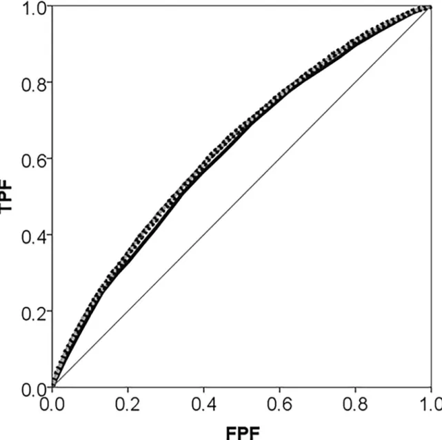
Fig 1. Areas under the receiver operating characteristic (AUC) curve for use of psychotropic drugs during 2006 in the city of Malmö, Sweden plotted separately for Model 1 which only adjusts for individual-level covariates age, sex and income (black thick line), and Model 2 which additionally adjust for neighbourhood of residence (grey dotted line).The diagonal line represents an AUC equal to 0.50.
characteristics, however, were not sufficient for predicting individuals’choice of GP with any degree of accuracy since the Model 1 AUC was low (i.e., 0.600).
Interestingly, the association between individual income and choosing a private GP declined when we recognized the multilevel structure of the data and included the neighbourhood level as a random effect in Model 2. This situation expresses the fact that the individual association in Model 1 was capturing not only a modest within neighbourhood association but also a stronger between neighbourhood association, A situation that was confirmed in Model 3 (see
under“Specific contextual average effects”) since the neighbourhood income was, on average,
strongly associated to choosing a private GP.
Specific contextual effects: IOR and POOR. Model 3 shows that high neighbourhood income was, on average, strongly associated with visiting a private physician (OR = 3.50). So the customary interpretation would be that, over and above individual income, age and sex, liv-ing in a high income neighbourhood strongly increased the individual probability of visitliv-ing a private physician. However, this contextual variable only explained a small share (PCV = 11%)
Fig 2. Predicted prevalence of psychotropic drug use in each neighborhood with 95% confidence intervals versus ranking.Predictions are for the reference individual in model 2, i.e.,female age 35–39, high income.
of the initially large neighbourhood variance. Therefore, unmodeled variability between neigh-bourhoods remained large as expressed by the wide IOR-80% = 0.09 -.130.28 Also the POOR indicated that 33% of the time an individual from a high income neighbourhood had a lower, rather that higher, likelihood of visiting a private GP than an individual from a low income neighbourhood. That is, the average OR hides strong heterogeneity around the average association.
General Contextual Effects: Neighbourhood variance, ICC, MOR and AUC. If the
neighbourhood context were relevant for understanding individuals’choice of private vs public
GPs we would expect a high ICC, a high MOR and a high increase of the AUC in Model 2 com-pared to Model 1. This is just what we found. The ICC in Model 2 was close to 60% and the
MOR close to 8 which are very high values in“neighbourhood and health”studies.
Further-more, adding information on neighbourhood in Model 2 increased the AUC of Model 1 from
Fig 3. Predicted prevalence of psychotropic drug use in each neighborhood with 95% confidence intervals versus ranking.Predictions are for the reference individual in model 3, i.e., female, age 35–39, high income and living in a high income neighborhood (model 3).
about 0.6 to almost 0.9 which indicates that knowing the neighbourhood of one’s residence allows us to predict with rather high accuracy if an individual will choose a private versus a
public GP (seeFig 4).
If the large observed general neighbourhood effect were mediated by neighbourhood income (or by other unobserved neighbourhood characteristics that this covariate may proxy for) we would expect a considerable reduction of the neighbourhood variance, the ICC, and the MOR in Model 3 compared with Model 2. However, this was not the case. In support of this argument, measuring the AUC using only individual variables and neighbourhood income but
not the neighbourhood random effect gave an AUC (95% confidence interval) = 0.620 (0.614–
0.626) which is only 0.03 units higher that Model 1 with only individual level variables.
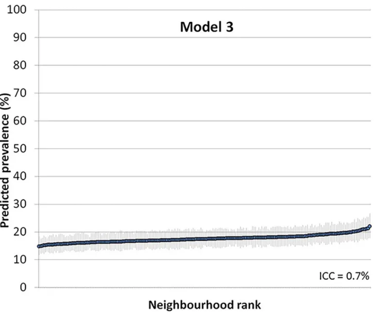
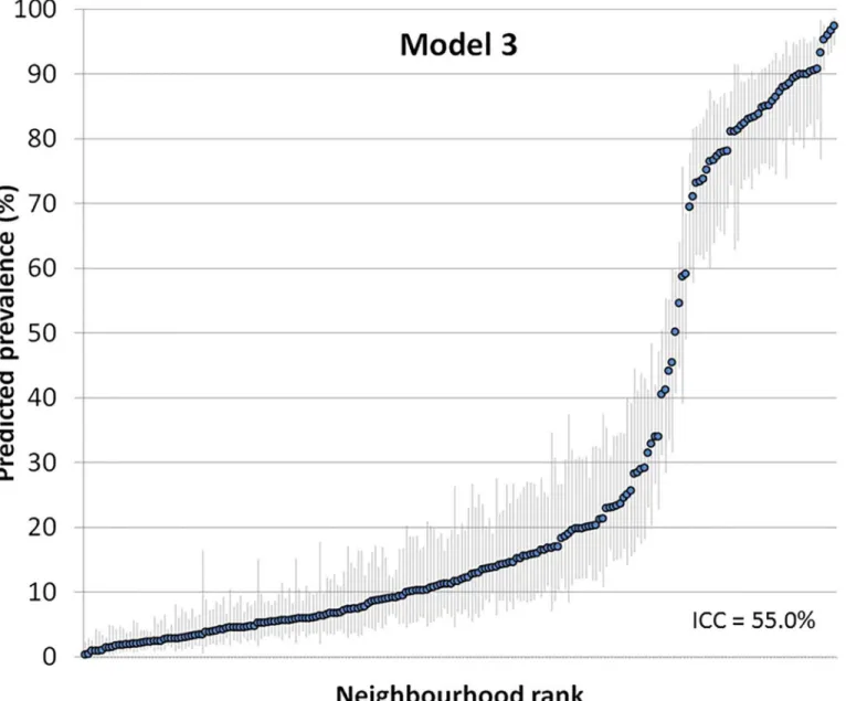
Figs5and6show the ranking of the neighbourhoods of Malmö in 2006 according to their
predicted prevalence of using a private physician in each neighborhood with 95% confidence
intervals versus ranking. Predictions are for the reference individual, i.e., female, age 35–39,
low income (model 2) and also living in a low income neighborhood (model 3).
Table 3. Multilevel logistic regression analysis of choosing a private versus a public specialist in the 35–65 year-old population of Malmö, 2006, Values are odds ratios (OR) and 95% confidence interval (CI) unless stated otherwise.
Simple logistic regression analysis Multilevel logistic regression analysis
Model 1 Model 2 Model 3
Specific individual average effects
Men vs. women 0.96 (0.92–1.01) 0.94 (0.88–1.01) 0.94 (0.88–1.01)
Age groups
35–39 Reference
40–44 1.01 (0.93–1.09) 1.07 (0.94–1.20) 1.07 (0.94–1.20)
45–49 1.02 (0.94–1.11) 1.22 (1.07–1.37) 1.22 (1.07–1.37)
50–54 1.08 (1.00–1.17) 1.25 (1.10–1.41) 1.25 (1.10–1.41)
55–59 1.21 (1.12–1.31) 1.30 (1.16–1.46) 1.30 (1.16–1.46)
60–64 1.20 (1.10–1.30) 1.20 (1.06–1.35) 1.20 (1.06–1.35)
High vs. low income 2.13 (2.02–2.24) 1.14 (1.06–1.22) 1.13 (1.04–1.22)
Specific contextual average effects
High vs. low neighbourhood income 3.50 (2.13–5.78)
80% IOR 0.09–130.28
POOR (%) 33
General contextual effects*
Neighbourhood variance 4.479 (3.699–5.502) 3.980 (3.277–4.892)
PCV (%) 11
ICC (%) 57.8 (53.1–62.7) 54.9 (50.1–59.9)
MOR 7.53 (6.42–9.37) 6.71 (5.62–8.25)
AUC 0.600 (0.593–0.606) 0.895 (0.891–0.899) 0.895 (0.891–0.899)
AUC change* 0.295 0.000
Goodness offit
DIC 44726 24647 24648
DIC change* -20079 1.28
IOR: interval odds ratio. POOR: proportion of opposed odds ratios. PCV: proportional change in the variance. ICC: intra-class correlation coefficient. MOR: median odds ratio. AUC: area under the receiver operating characteristic curve. DIC: Bayesian diagnostic information criterion.
*: change in relation to the previous model
We observed a bimodal distribution for the neighbourhood differences with two groups of neighbourhoods, one smaller group with a higher probability of visiting a private GP, and another larger group with a lower probability. This bimodality reflects the underlying nature of private GP use. In our case, it revealed that over and above age, sex and individual income, individuals in some neighbourhoods mostly visit private physicians while individuals in other neighbourhoods mostly visit public GPs. A similar bimodality is frequently observed when there are strong general contextual effects in other settings as is the case when analysing
indi-vidual within households [4,49], sibling within families [50], or children within mothers [51].
This bimodality was not a concern for the statistical analysis as the number of neighbour-hoods was high, which makes the assumption of normally distributed random effects less
rele-vant [52]. Nevertheless, adjusting for neighbourhood income (low vs high) reduced the
bimodality and it is assumable that the bimodality might be further reduced by modelling
Fig 4. Areas under the receiver operating characteristic curve (AUC) for choosing a private vs. a public GP during 2006 in the city of Malmö, Sweden plotted separately for Model 1 which only adjusts for individual-level covariates age, gender and income (black thick line); and for Model 2 which additionally adjusts for the neighbourhood of residence (grey dotted line).The diagonal line represents an AUC equal to 0.50.
neighbourhood income in a more flexibly way (e.g., by entering a continuous measure of neigh-bourhood income as a polynomial). The pattern of neighneigh-bourhood differences also suggests the existence of spatial correlation which could be conditioned by the segregation of private practices in specific geographical areas. It is possible to allow for spatially correlated random effects in multilevel logistic regression, but this is beyond the scope of the current article.
We also note that there was high individual socioeconomic segregation. Multilevel logistic regression analyses have recently been proposed for modelling social and other forms of
segre-gation [53–55]. Applying those ideas to our data, we fit a separate multilevel logistic regression
analyses, modelling low individual income as the response variable. We estimated a neighbour-hood variance of 1.032 which corresponds to an ICC of 24% and substantial segregation. Therefore, adjusting neighbourhood income for individual income is to some extent based on
Fig 5. Predicted prevalence of using a private physician in each neighborhood with 95% confidence intervals versus ranking.Predictions are for the reference individual in model 2, i.e., female, age 35–39, low income.
extrapolations since there are relatively few individuals with high income living in poor
neigh-bourhoods and relatively few individuals with low income living in rich neighneigh-bourhoods.[56]
Discussion
We have presented two applications illustrating how to use multilevel logistic regression analy-sis of heterogeneity to estimate individual and neighbourhood influences on individual health and health care utilization. Our three-step approach distinguishes between specific (measures of association) and general (measures of variance) contextual effects, and demonstrates the rel-evance of combining both approaches for gaining greater substantive understanding of the phenomenon under study. We analyse two different individual outcomes (psychotropic drug use and visit to a private vs. public GP) for which the relative importance of neighbourhood
Fig 6. Predicted prevalence of using a private physician in each neighborhood with 95% confidence intervals versus ranking.Predictions are for the reference individual in model 3, i.e., female, age 35–39, low income and living in a low income neighborhood.
influences differs substantially. Our results agree with previous studies on the city of Malmö observing a large general neighbourhood effect for individual choice of private physician in
1999 (i.e., ICC = 33%, MOR = 3.36) [29] but a minor general neighbourhood effect for use of
anxiolytic-hypnotic drugs (i.e., ICC = 1.7%, MOR = 1.25) in 1991–1996 [57].
We question the current probabilistic, risk factor epidemiological approach based on the sim-ple interpretation of ORs for specific individual and contextual (e.g., neighbourhood)
character-istics in isolation [2]. We promote a three-step multilevel analytical approach. Step 1 consists of
fitting a single-level logistic regression adjusting for only the individual-level covariates, then evaluating the ORs and calculating the discriminatory accuracy (e.g., AUC) of these variables. Step 2 consists of extending the model to two-levels (by adding the neighbourhood random effect) and then assessing the importance of general contextual effects using the ICC and AUC. Step 3 consists of adding specific neighbourhood characteristics (i.e., specific neighbourhood effects) to the model and interpreting their ORs jointly with the size of the initial general contex-tual effect and the size of the neighbourhood variance explained (i.e., PCV). We argue that the incorrect population average interpretation of the OR for contextual variables needs be avoided. For this purpose the IOR or the POOR should be presented side-by-side with the average OR.
Psychotropic drug use
Applying our three-step approach to psychotropic drug use, we observed that sex, increased age, and individual low income were associated with the use of this medication. However, the information provided by these individual characteristics did not allow users of psychotropic drugs to be distinguished from non-users with any degree of accuracy (AUC = 0.616). We also observed a very small general contextual effect since accounting for neighbourhood of resi-dence only increased the AUC by 0.014 units and both the ICC (i.e., 1.1%) and the MOR (i.e., 1.20) were very low. In fact, our results suggest that SAMS neighbourhoods were more similar to simple random samples from the population of Malmö, than to meaningful contexts influ-encing individual psychotropic drug use.
The low AUC of the neighbourhood context (i.e., the low general contextual effects) needs to be considered when interpreting the small but conclusive association between low bourhood income and individual use of psychotropic drugs. One could argue that this neigh-bourhood variable explained 42% of the neighneigh-bourhood variance, but as such variance was
rather small (i.e.,s^2
u= 0.038), it actually explained a lot of very little. Furthermore, the POOR
informed that 11% of the time the positive association between low neighbourhood income and individual psychotropic drug use was in the opposite direction with a decreased, rather than increased, propensity of using psychotropic drugs in the low income neighbourhoods.
Paradoxically, when the neighbourhood variance is low (i.e., there is a weak general
contex-tual effect) it is easier to obtain“significant”associations with narrow 95% CI for the contextual
variables (i.e., specific contextual effect). This situation happens because we assign the values of neighbourhood variable to uncorrelated individuals in the sample. In other words, the less
neighbourhood boundaries matter for the outcome, the easier it is to get“significant”
associa-tions between specific neighbourhood characteristics and the individual outcome. When
researchers plan a study of“neighbourhood and health”, they typically assume that there is a
strong intra-neighbourhood correlation. However, we need to check this assumption and always interpreted the specific contextual effect (i.e., OR and 95% confidence interval) consid-ering the size of the initial general contextual effects (e.g., ICC or AUC). Following the three-stage approach promoted in this article ensures a more appropriate interpretation.
Care centres where the individuals are treated. The SAMS areas were relatively easy to obtain but their definition was not based on robust theory related to the contextual processes and mechanisms that may condition use of psychotropic drugs (or, for that matter, the choice of a private GP). In fact, the relevant context may not be at the neighbourhood level at all.
Prescrip-tion of psychotropic drugs is homogenously regulated all over Sweden [58], which may reduce
the influence of the neighbourhood on individual use of this medication. However, larger con-textual effects might be observed when studying countries with different health care systems and therapeutic traditions or where psychotropic drugs are available over the counter. We have previously observed such a situation in the context of studying blood pressure. We identified a
very low general contextual effect of the city areas in Malmö [10], but this effect was much
higher when analysing countries with different health care systems [11]
In summary, we were not able to identify with accuracy the factors that predict psychotropic drug use. What we did find was that individual age, sex, and low income appeared to be poor predictors for identifying users of psychotropic drugs, and additionally including neighbour-hood of residence did not alter this situation. That is, the neighbourneighbour-hood context had only a negligible influence on individual use of psychotropic drugs.
Choice of a private vs. a public GP
Concerning individual choice of private vs. public GP, our analysis showed that while the sex of the individual was not related to this choice, age was weakly positively associated and individual high income strongly associated (OR = 2.13) to this choice. However, as in the case of psycho-tropic drug use, the low discriminatory accuracy (AUC = 0.600) rendered the information sup-plied by these individual-level covariates insufficient for distinguishing who would choose a private vs. public GP. However, we found a very strong general contextual effect since account-ing for neighbourhood of residence in the analysis increased by 0.295 units the AUC to 0.895. Also, the large ICC (i.e., 57.8%) and MOR (i.e., 7.53) values indicate that SAMS neighbourhoods captured a meaningful context influencing this individual behaviour. The socioeconomic con-text of the neighbourhoods (i.e., high vs. low neighbourhood income) was, on average, associ-ated with choosing a private GP (OR = 3.50). However, this specific neighbourhood variable
only explained 11% of the large neighbourhood variance in Model 2 (i.e.,s^2
u= 4.479). In fact, in
as much as 33% of comparisons between rich and poor neighbourhoods, the OR for neighbour-hood income was in the opposite direction so high neighbourneighbour-hood income was associated to a lower rather than a higher propensity of choosing a private GP.
of having a positive response. However, the fact remains that 89% of the neighbourhood vari-ance still persits unexplained and is attributed, collectively, to other unmodeled factors. Whether any of these unobserved factors individually explains a much higher proportion of the neighbourhood variance we can only speculate.
We observed that, on average, utilization of private GPs was higher among high income people and in high income neighbourhoods than in the low income categories, which deserves
a closer analysis. In fact, access to health care in Sweden is by law [59] on equal terms and
according to needs, and for many years societal funding has equally financed both public and
private health [60] so economic circumstances should not be the main reason for choosing a
public vs. a private GP [60]. The observed link between income and utilization of private GPs
might depend on cultural preferences rather than solely on economic reasons. It is known, for
example, that choice of sector also carries a symbolic meaning [61] and high income
individu-als have been argued to intrinsically prefer private care. However, an alternative explanation
could be the existence of“invisible”barriers like adverse attitudes of private GPs against low
income individuals, which might channel those individuals towards public GPs [60].
In summary, neither the simple comparison of the proportion of individuals visiting a private GP in rich vs. poor areas (35% vs 11% respectively) nor the OR of the neighbourhood variable inform of the discriminatory accuracy of the income variable. Rather the multilevel analysis including the AUC as a measure of discriminatory accuracy informed that over and above indi-vidual characteristics the neighbourhood of residence strongly predicted the choice of a private vs. a public GP, but the reasons for this phenomenon are only partially explained by socioeco-nomic circumstances of the neighbourhoods. On average, individuals residing in high income neighbourhoods had a higher propensity of visiting a private GP, but this contextual variable only explained a low proportion of the variation in neighbourhood differences. Other contextual factors not considered in our analysis, for instance, the degree of private GP provision in each neighbourhood might go some way to explaining the observed general contextual effects.
Public Health implications
According to our analyses, policies to improve psychological health or reduce the use of psy-chotropic drugs in the city of Malmö would need to realize that focusing on specific neighbour-hoods would not be effective because of the low discriminatory accuracy of this information. In fact, the same is true for the individual characteristics we analysed: age, sex, and income. Put differently, neither neighbourhood of residence nor the individual characteristics studied pro-vided accurate information for identifying target groups. If policy makers do choose to focus on those individuals and neighbourhood with a higher average risk of using psychotropic drugs (which would be the normal procedure in risk factors epidemiology), they need to be
aware that many psychotropic users would be labelled as“low risk”and that many non-users
of psychotropic drugs would be labelled as“high-risk”. That is, focusing on only high risk
groups would unnecessarily expose many individuals to an intervention they do not need and would leave many individuals untreated because they belong to low risk groups. Perhaps a bet-ter approach would be to launch an inbet-tervention on the whole population. In any case, consid-ering the balance between harms and benefits, an intervention with low discriminatory
accuracy conveys that the principle ofprimum non noceremust be an absolute condition.
The public health implications of our second analysis are very different. Here, policies to increase the use of public GP services should mostly focus on specific neighbourhoods, perhaps by opening local public GP alternatives.
choice of GP in particular. However, our primary aim was to illustrate how to perform and interpret a multilevel analysis of individual heterogeneity in social epidemiology and public health so we only considered a few variables. In any case, our study shows that neighbourhood
“effects”are not properly quantified by differences between neighbourhood averages but rather
by measuring the share of the individual heterogeneity that exists at the neighbourhood level.
Multilevel analysis of heterogeneity and risk factors epidemiology
The multilevel analysis of heterogeneity we present in our study is rather innovative [2]. Most
studies analysing the role of individual or contextual variables on health adopt a probabilistic perspective based on the analysis of differences in average risk between exposed and unexposed
groups [62] but without recognizing the value of analysing variance [63]. This is the classical
approach in so called“risk factors epidemiology”and many multilevel analyses have only
focused on the identification of contextual risk factors such as neighbourhood social capital and neighbourhood deprivation. From this perspective small or even tiny effects (e.g., OR = 1.5 or even lower) with very low discriminatory accuracy are considered relevant. The problem is that by doing so we promote population level policies and interventions that may lead to both under and overtreatment, as well as unnecessary side effects and costs. It also raises ethical con-cerns related to misleading risk communication and the perils of both unwarranted
interven-tions and stigmatization of exposed individuals[2,64].
The multilevel analytical approach we propose differs fundamentally from the classical one. First, we adopt a mechanistic perspective that tries to understand the individual heterogeneity of responses surrounding average probabilities. Second, we combine measures of association with measures of variance and discriminatory accuracy and stress the importance of evaluating not only the discriminatory accuracy of the individual level variables but also of the geographi-cal boundaries used to define neighbourhoods in relation to the outcome under investigation.
For this purpose what we denominatedgeneral contextual effectsin multilevel regression
analy-sis allows us to quantify the degree of clustering within neighbourhoods (i.e., the ICC) [7,14]
or, analogously, the discriminatory accuracy of using the boundaries of the neighbourhoods in
the analysis (i.e., the AUC) [33,34]. The existence of individual dependence within
neighbour-hoods is not only thesine qua nonfor applying statistical multilevel analyses but also the size
of this dependence provides fundamental substantive information [2,3].
Strength and weaknesses
Our current study tries to quantify the relevance of neighbourhoods in Malmö for understand-ing individual use of psychotropic drugs and choice of private vs public GP. We considered the simplest possible multilevel structure of individual nested within neighbourhoods as this is the most common design in neighbourhood and health studies. However, to constrain the study of contextual effects to a single geographical level (e.g., SAMS areas) is certainly an extreme
sim-plification [65]. Individuals are likely to be simultaneously affected by multiple contexts at
dif-ferent scales across time [66–70]. Besides, other kind of contexts like the household are
normally disregarded in studies of neighbourhood and health [4] [49]. Nevertheless, the
analyt-ical approach we promote can be developed for more than two levels of analyses (e.g.,
individu-als nested in households nested in neighbourhoods) [4] as well as for multiple membership
and cross-classified multilevel structures (e.g., schools and neighbourhoods at different times
in the life course) [2,67,71–73]. However, adopting a pragmatic rather than academic
simple ecological or spatial analyses of small area variation or classical multilevel analysis of
contextual risk factors [4].
The identification of causal effects in observational epidemiology and, more specifically, in
the study of neighbourhoods“effects”is a major problem. In our study, the underlying causal
question was to know what would happen to an individual if she/he,ceteris paribus, moves to
another neighbourhood with a different context. Furthermore, we wanted to identify if any general effect was mediated by a specific variable informing the socioeconomic characteristics
of the context (e.g., rich vs. poor neighbourhood). However, what“rich”and“poor”
neighbour-hood means is difficult to specify and it would need a deeper sociological analysis. In the adjusted analysis we only considered individual age, sex and income as our main purpose was to illustrate the methodology. Therefore, we cannot exclude the existence of omitted confound-ing factors. Nevertheless, in neighbourhood analyses it is always a caveat to distconfound-inguish between confounder and mediator variables as frequently a common cause of both place of residence and the health outcome may also be a mediator of the neighbourhood effect (for instance low income is associated to using psychotropic drugs and low income individuals may be segre-gated to poor neighbourhoods but, in turn, living in a poor neighbourhood may reduce the
chances of increasing an individual’s income). Furthermore, there may be problems of
extrapo-lation (i.e., making inferences beyond the range of the data,) since few rich individuals reside in poor neighbourhoods and vice versa, so the appropriateness of adjusting for individual income could be questioned. Finally, while some contextual effects may be caused by exogenous expo-sures (e.g., absence of public GPs in an area) other may be endogenous and emerge from the individual composition of the neighbourhood (e.g., switching all low and high income individ-uals to rich and low neighbourhood will also change the neighbourhood context). In general, drawing valid causal inferences in observational epidemiology is difficult and this is especially
the case in neighbourhood and health studies [2,56].
Correspondence between the different measures used to estimate
general contextual effects
When using model predictions that include a random intercept [74,75], as in the present
study, there is a clear correspondence between the ICC and the AUC. That is, when the ICC is high the AUC is also high. However, under certain circumstances like when the number of individuals is relatively much larger in some neighbourhood than in others and/or if the num-ber of neighbourhood is low, it could be possible to find a discrepancy between the ICC and the AUC (for instance the ICC may be high but the AUC low). The reason for this discrepancy is that the calculation of the ICC is based on the neighbourhood variance which, in turn, is
based on differences between neighbourhoods’averages and it is, therefore, standardized for
neighbourhood size (i.e., the number of individuals in the neighbourhoods). On the other hand, the AUC is based on the calculation of the TPF and FPF for different thresholds of the predicted probability. Since this predicted probability is an individual level variable, large clus-ters contribute with more individuals. In other words, the AUC measure is a weighted average of a within- and a between-cluster part of the individual predictions, where the ICC measure is
based on the neighbourhood variance (i.e., random effects) only [75]. This situation does not
mean that the AUC is a biased measure but, rather, it provides different and useful
informa-tion. For instance, some large neighbourhoods could have ahighproportion of individuals
vis-iting a private GP and some small neighbourhoods could have alowproportion of individuals