www.hydrol-earth-syst-sci.net/20/4775/2016/ doi:10.5194/hess-20-4775-2016
© Author(s) 2016. CC Attribution 3.0 License.
The evolution of root-zone moisture capacities after deforestation:
a step towards hydrological predictions under change?
Remko Nijzink1, Christopher Hutton2, Ilias Pechlivanidis4, René Capell4, Berit Arheimer4, Jim Freer2,3, Dawei Han2, Thorsten Wagener2,3, Kevin McGuire5, Hubert Savenije1, and Markus Hrachowitz1
1Water Resources Section, Faculty of Civil Engineering and Geosciences, Delft University of Technology,
Stevinweg 1, 2628 CN Delft, the Netherlands
2Department of Civil Engineering, University of Bristol, Bristol, UK 3Cabot Institute, University of Bristol, Bristol, UK
4Swedish Meteorological and Hydrological Institute (SMHI), Norrköping, Sweden
5Virginia Water Resources Research Center and Department of Forest Resources and Environmental
Conservation, Virginia Tech, Blacksburg, VA, USA Correspondence to:Remko Nijzink (r.c.nijzink@tudelft.nl)
Received: 21 August 2016 – Published in Hydrol. Earth Syst. Sci. Discuss.: 29 August 2016 Revised: 5 November 2016 – Accepted: 11 November 2016 – Published: 5 December 2016
Abstract. The core component of many hydrological sys-tems, the moisture storage capacity available to vegetation, is impossible to observe directly at the catchment scale and is typically treated as a calibration parameter or obtained from a priori available soil characteristics combined with estimates of rooting depth. Often this parameter is considered to re-main constant in time. Using long-term data (30–40 years) from three experimental catchments that underwent signifi-cant land cover change, we tested the hypotheses that: (1) the root-zone storage capacity significantly changes after defor-estation, (2) changes in the root-zone storage capacity can to a large extent explain post-treatment changes to the hy-drological regimes and that (3) a time-dynamic formulation of the root-zone storage can improve the performance of a hydrological model.
A recently introduced method to estimate catchment-scale root-zone storage capacities based on climate data (i.e. ob-served rainfall and an estimate of transpiration) was used to reproduce the temporal evolution of root-zone storage capac-ity under change. Briefly, the maximum deficit that arises from the difference between cumulative daily precipitation and transpiration can be considered as a proxy for root-zone storage capacity. This value was compared to the value ob-tained from four different conceptual hydrological models that were calibrated for consecutive 2-year windows.
It was found that water-balance-derived root-zone storage capacities were similar to the values obtained from calibra-tion of the hydrological models. A sharp decline in root-zone storage capacity was observed after deforestation, followed by a gradual recovery, for two of the three catchments. Trend analysis suggested hydrological recovery periods between 5 and 13 years after deforestation. In a proof-of-concept anal-ysis, one of the hydrological models was adapted to allow dynamically changing root-zone storage capacities, follow-ing the observed changes due to deforestation. Although the overall performance of the modified model did not consider-ably change, in 51 % of all the evaluated hydrological signa-tures, considering all three catchments, improvements were observed when adding a time-variant representation of the root-zone storage to the model.
1 Introduction
Vegetation, as a core component of the water cycle, shapes the partitioning of water fluxes on the catchment scale into runoff components and evaporation, thereby controlling fun-damental processes in ecosystem functioning (Rodriguez-Iturbe, 2000; Laio et al., 2001; Kleidon, 2004), such as flood generation (Donohue et al., 2012), drought dynamics (Seneviratne et al., 2010; Teuling et al., 2013), groundwater recharge (Allison et al., 1990; Jobbágy and Jackson, 2004) and land–atmosphere feedback (Milly and Dunne, 1994; Seneviratne et al., 2013; Cassiani et al., 2015). Besides in-creasing interception storage available for evaporation (Ger-rits et al., 2010), vegetation critically interacts with the hy-drological system in a co-evolutionary way by root water up-take for transpiration, towards a dynamic equilibrium with the available soil moisture to avoid water shortage (Dono-hue et al., 2007; Eagleson, 1978, 1982; Gentine et al., 2012; Liancourt et al., 2012) and related adverse effects on car-bon exchange and assimilation rates (Porporato et al., 2004; Seneviratne et al., 2010). Roots create moisture storage vol-umes within their range of influence, from which they extract water that is stored between field capacity and wilting point. This root-zone storage capacitySR, sometimes also referred
to as plant available water holding capacity, in the unsatu-rated soil is therefore the key component of many hydrologi-cal systems (Milly and Dunne, 1994; Rodriguez-Iturbe et al., 2007).
There is increasing theoretical and experimental evidence that vegetation dynamically adapts its root system, and thus SR, to environmental conditions, to secure, on the one hand,
access to sufficient moisture to meet the canopy water de-mand and, on the other hand, to minimize the carbon in-vestment for sub-surface growth and maintenance of the root system (Brunner et al., 2015; Schymanski et al., 2008; Tron et al., 2015). In other words, the hydrologically active root zone is optimized to guarantee productivity and transpira-tion of vegetatranspira-tion, given the climatic circumstances (Klei-don, 2004). Several studies previously showed the strong in-fluence of climate on this hydrologically active root zone (e.g. Reynolds et al., 2000; Laio et al., 2001; Schenk and Jackson, 2002). Moreover, droughts are often identified as critical situations that can affect ecosystem functioning evo-lution (e.g. Allen et al., 2010; McDowell et al., 2008; Vose et al., 2016).
In addition to their general adaption to environmental con-ditions, vegetation has some potential to adapt roots to such periods of water shortage (Sperry et al., 2002; Mencuccini, 2003; Bréda et al., 2006). In the short term, stomatal clo-sure and reduction of leaf area will lead to reduced tran-spiration. In several case studies for specific plants, it was also shown that plants may even shrink their roots and re-duce soil–root conductivity during droughts, while recover-ing after re-wettrecover-ing (Nobel and Cui, 1992; North and No-bel, 1992). In the longer term, and more importantly, trees
can improve their internal hydraulic system, for example by recovering damaged xylem or by allocating more biomass for roots (Sperry et al., 2002; Rood et al., 2003; Bréda et al., 2006). Similarly, Tron et al. (2015) argued that roots fol-low groundwater fluctuations, which may lead to increased rooting depths when water tables drop. Such changing envi-ronmental conditions may also provide other plant species with different water demand than the ones present under given conditions, with an advantage in the competition for resources, as for example shown by Li et al. (2007).
The hydrological functioning of catchments (Black, 1997; Wagener et al., 2007) and thus the partitioning of water into evaporative fluxes and runoff components is not only af-fected by the continuous adaption of vegetation to chang-ing climatic conditions. Rather, it is well understood that anthropogenic changes to land cover, such as deforestation, can considerably alter hydrological regimes. This has been shown historically through many paired watershed studies (e.g. Bosch and Hewlett, 1982; Andréassian, 2004; Brown et al., 2005; Alila et al., 2009). These studies found that defor-estation often leads to generally higher seasonal flows and/or an increased frequency of high flows in streams, while de-creasing evaporative fluxes. The timescales of hydrological recovery after such land-cover disturbances were shown to be highly sensitive to climatic conditions and the growth dy-namics of the regenerating species (e.g. Jones and Post, 2004; Brown et al., 2005).
Although land-use change effects on hydrological func-tioning are widely acknowledged, it is less well understood which parts of the hydrological system are affected in which way and over which timescales. As a consequence, most catchment-scale models were originally not developed to deal with such changes in the system, but rather for “station-ary” conditions (Ehret et al., 2014). This is true for both top-down hydrological models, such as HBV (Bergström, 1992) or GR4J (Perrin et al., 2003), and bottom-up models, such as MIKE-SHE (Refsgaard and Storm, 1995) or HydroGeo-Sphere (Brunner and Simmons, 2012). Several modelling studies have in the past incorporated temporal effects of land-use change to some degree (Andersson and Arheimer, 2001; Bathurst et al., 2004; Brath et al., 2006), but they mostly rely on ad hoc assumptions about how hydrological parameters are affected (Legesse et al., 2003; Mahe et al., 2005; On-stad and Jamieson, 1970; Fenicia et al., 2009). Approaches which incorporate the change in the model formulation itself are rare and have only recently gained momentum (e.g. Du et al., 2016; Fatichi et al., 2016; Zhang et al., 2016). This is of critical importance as ongoing changes in land cover and climate dictate the need for a better understanding of their effects on hydrological functioning (Troch et al., 2015) and their explicit consideration in hydrological models for more reliable predictions under change (Hrachowitz et al., 2013; Montanari et al., 2013).
Table 1.Overview of the catchments and their sub-catchments (WS).
Catchment Deforestation Treatment Area Affected Aridity Precipitation Discharge Potential Time series period [km2] Area [%] index [–] [mm yr−1] [mm yr−1] evaporation
[mm yr−1]
HJ Andrews WS1 1962–1966 Burned 1966 0.956 100 0.39 2305 1361 902 1962–1990
HJ Andrews WS2 – – 0.603 – 0.39 2305 1251 902 1962–1990
Hubbard Brook WS2 1965–1968 Herbicides 0.156 100 0.57 1471 1059 784 1961–2009
Hubbard Brook WS3 – – 0.424 – 0.54 1464 951 787 1961–2009
Hubbard Brook WS5 1983–1984 No treatment 0.219 87 0.51 1518 993 746 1962–2009
root-zone storage capacity, SR, is a core component
deter-mining the hydrological response, and needs to be treated as a dynamically evolving parameter in hydrological modelling as a function of climate and vegetation. Gao et al. (2014) re-cently demonstrated that catchment-scaleSRcan be robustly
estimated exclusively based on long-term water balance con-siderations. Wang-Erlandsson et al. (2016) derived global es-timates ofSRusing remote-sensing based precipitation and
evaporation products, which demonstrated considerable spa-tial variability ofSR in response to climatic drivers. In
tra-ditional approaches,SRis typically determined either by the
calibration of a hydrological model (e.g. Seibert and McDon-nell, 2010; Seibert et al., 2010) or based on soil characteris-tics and sparse, averaged estimates of root depths, often ob-tained from literature (e.g. Breuer et al., 2003; Ivanov et al., 2008). This does neither reflect the dynamic nature of the root system nor does it consider to a sufficient extent the ac-tual function of the root zone: providing plants with contin-uous and efficient access to water. This leads to the situation where soil porosity often effectively controls the values of SRused in a model. Consider, as a thought experiment, two
plants of the same species growing on different soils. They will, with the same average root depth, then have access to different volumes of water, which will merely reflect the dif-ferences in soil porosity. This is in strong contradiction to the expectation that these plants would design root systems that provide access to similar water volumes, given the evi-dence for efficient carbon investment in root growth (Milly, 1994; Schymanski et al., 2008; Troch et al., 2009) and posing that plants of the same species have common limits of oper-ation. This argument is supported by a recent study, in which was shown that water-balance-derived estimates ofSRare at
least as plausible as soil-derived estimates (de Boer-Euser et al., 2016) in many environments and that the maximum root depth controls evaporative fluxes and drainage (Camporese et al., 2015).
Therefore, using water-balance-based estimates ofSR in
several deforested sites as well as in untreated reference sites in two experimental forests, we test the hypotheses that (1) the root-zone storage capacity SR significantly changes
after deforestation, (2) the evolution inSRcan explain
post-treatment changes to the hydrological regimes and that (3) a
time-dynamic formulation of SR can improve the
perfor-mance of a hydrological model.
2 Study sites
The catchments under consideration are part of the HJ An-drews Experimental Forest and the Hubbard Brook Experi-mental Forest. A summary of the main catchment character-istics can be found in Table 1. Daily discharge (Campbell, 2014a; Johnson and Rothacher, 2016), precipitation (Camp-bell, 2014b; Daly and McKee, 2016) and temperature time series (Campbell, 2014c, d; Daly and McKee, 2016) were obtained from the databases of the Hubbard Brook Experi-mental Forest and the HJ Andrews ExperiExperi-mental Forest. Po-tential evaporation was estimated by the Hargreaves equation (Hargreaves and Samani, 1985).
2.1 HJ Andrews Experimental Forest
The HJ Andrews Experimental Forest is located in Oregon, USA (44.2◦N, 122.2◦W) and was established in 1948. The catchments at HJ Andrews are described in many studies (e.g. Rothacher, 1965; Dyrness, 1969; Harr et al., 1975; Jones and Grant, 1996; Waichler et al., 2005).
Before vegetation removal and at lower elevations the for-est generally consisted of 100- to 500-year old coniferous species, such as Douglas fir (Pseudotsuga menziesii), west-ern hemlock (Tsuga heterophylla) and western red cedar (Thuja plicata), whereas upper elevations were characterized by noble fir (Abies procera), Pacific silver fir (Abies ama-bilis), Douglas fir, and western hemlock. Most of the precip-itation falls from November to April (about 80 % of the an-nual precipitation), whereas the summers are generally drier, leading to signals of precipitation and potential evaporation that are out of phase.
2.2 Hubbard Brook Experimental Forest
The Hubbard Brook Experimental Forest is a research site established in 1955 and located in New Hampshire, USA (43.9◦N, 71.8◦W). The Hubbard Brook experimental catch-ments are described in a many publications (e.g. Hornbeck et al., 1970, 1997; Hornbeck, 1973; Dahlgren and Driscoll, 1994; Likens, 2013).
Prior to vegetation removal, the forest was dominated by northern hardwood forest composed of sugar maple (Acer saccharum), American beech (Fagus grandifolia) and yellow birch (Betula alleghaniensis) with conifer species such as red spruce (Picea rubens) and balsam fir (Abies balsamea) oc-curring at higher elevations and on steeper slopes with shal-low soils. The forest was selectively harvested from 1870 to 1920, damaged by a hurricane in 1938, and is currently not accumulating biomass (Campbell et al., 2013; Likens, 2013). The annual precipitation and runoff is less than in HJ Andrews (Table 1). Precipitation is rather uniformly spread throughout the year without distinct dry and wet periods, but with snowmelt-dominated peak flows occurring around April and distinct low flows during the summer months due to in-creased evaporation rates (Federer et al., 1990). Vegetation removal occurred in the catchment of Hubbard Brook WS2 between 1965 and 1968 and in Hubbard Brook Watershed 5 (WS5) between 1983 and 1984. Hubbard Brook Watershed 3 (WS3) is the undisturbed reference catchment.
Hubbard Brook WS2 was completely deforested in November and December 1965 (Likens et al., 1970). To min-imize disturbance, no roads were constructed and all timber was left in the catchment. On 23 June 1966, herbicides were sprayed from a helicopter to prevent regrowth. Additional herbicides were sprayed in the summers of 1967 and 1968 from the ground.
In Hubbard Brook WS5, all trees were removed between 18 October 1983 and 21 May 1984, except for a 2 ha buffer near an adjacent reference catchment (Hornbeck et al., 1997). WS5 was harvested as a whole-tree mechanical clearcut with removal of 93 % of the above-ground biomass (Hornbeck et al., 1997; Martin et al., 2000), thus including smaller branches and debris. Approximately 12 % of the catchment area was developed as the skid trail network. Afterwards, no treatment was applied and the site was left for regrowth.
3 Methodology
To assure reproducibility and repeatability, the executional steps in the experiment were defined in a detailed protocol, following Ceola et al. (2015), which is provided as Supple-ment Sect. S1.
Table 2.Applied parameter ranges for root-zone storage derivation.
Catchment Imax,eq Imax,change Tr
(mm) (mm) (days)
HJ Andrews WS1 1–5 0–5 0–3650
HJ Andrews WS2 1–5 – –
Hubbard Brook WS2 1–5 5–10 0–3650
Hubbard Brook WS3 1–5 – –
Hubbard Brook WS5 1–5 0–5 0–3650
3.1 Water-balance-derived root-zone moisture capacitiesSR
The root-zone moisture storage capacities SR and their
change over time were determined according to the methods suggested by Gao et al. (2014) and subsequently successfully tested by de Boer-Euser et al. (2016) and Wang-Erlandsson et al. (2016). Briefly, the long-term water balance provides formation on actual mean transpiration. In a first step, the in-terception capacity has to be assumed, in order to determine the effective precipitationPe (L T−1), following the water
balance equation for interception storage: dSi
dt =P−Ei−Pe (1)
withSi (L) interception storage,P the precipitation (L T−1), Ei the interception evaporation (L T−1). This is solved with the constitutive relations:
Ei = ( E
p ifEpdt < Si Si
dt ifEpdt≥Si
(2)
Pe= (
0 ifSi≤Imax
Si−Imax
dt ifSi > Imax
(3)
with, additionally,Epthe potential evaporation (L T−1) and
Imax(L) the interception capacity. AsImax will also be
af-fected by land cover change, this was addressed by intro-ducing the three parametersImax,eq (long-term equilibrium
interception capacity) (L),Imax,change(post-treatment
inter-ception capacity) (L) andTr(recovery time) (T), leading to
a time-dynamic formulation ofImax:
Imax=
fort < tchange, t > tchange,end+Tr: Imax,eq
fortchange, start< t < tchange,end:
Imax,eq−
Imax,eq−Imax,change tchange,end−tchange,start
t−tchange,start
fortchange,end< t < tchange,end+Tr:
Imax,change+
Imax,eq−Imax,change Tr
t−tchange,end
Figure 1.Derivation of root-zone storage capacity (SR)for one spe-cific time period in Hubbard Brook WS2 as difference between the cumulative transpiration (Et)and the cumulative effective precipi-tation (PE).
withtchange,startthe time that deforestation started andtstart,end
the time deforestation finished.
Following a Monte Carlo sampling approach, upper and lower bounds ofEi were then estimated based on 1000 ran-dom samples of these parameters, eventually leading to up-per and lower bounds forPe. The interception capacity was
assumed to increase after deforestation for Hubbard Brook WS2, as the debris was left at the site. For Hubbard Brook WS5 and HJ Andrews WS1 the interception capacity was assumed to decrease after deforestation, as here the debris was respectively burned and removed. Furthermore, in the absence of more detailed information, it was assumed that the interception capacities changed linearly during deforesta-tion towards Imax,changeand linearly recovered toImaxover
the periodTras well. See Table 2 for the applied parameter
ranges.
Hereafter, the long-term mean transpiration can be esti-mated with the remaining components of the long term wa-ter balance, assuming no additional gains or losses, storage changes and/or data errors:
Et=Pe−Q, (5)
where Et (L T−1) is the long-term mean actual
transpira-tion,Pe(L T−1) is the long-term mean effective precipitation
andQ(L T−1) is the long-term mean catchment runoff. Tak-ing into account seasonality, the actual mean transpiration is scaled with the ratio of long-term mean daily potential evap-orationEpover the mean annual potential evaporationEp:
Et(t )=
Ep(t )
Ep
×Et. (6)
Based on this, the cumulative deficit between actual transpi-ration and precipitation over time can be estimated by means
of an “infinite-reservoir”. In other words, the cumulative sum of daily water deficits, i.e. evaporation minus precipitation, is calculated betweenT0, which is the time the deficit equals
zero, andT1, which is the time the total deficit returned to
zero. The maximum deficit of this period then represents the volume of water that needs to be stored to provide vegetation continuous access to water throughout that time:
SR=max T1 Z
T0
(Et−Pe)dt, (7)
whereSR (L) is the maximum root-zone storage capacity
over the time period between T0 and T1. See also Fig. 1
for a graphical example of the calculation for the Hubbard Brook catchment for one specific realization of the parameter sampling. TheSR,20yrfor drought return periods of 20 years
was estimated using the Gumbel extreme value distribution (Gumbel, 1941) as previous work suggested that vegetation designsSRto satisfy deficits caused by dry periods with
re-turn periods of approximately 10–20 years (Gao et al., 2014; de Boer-Euser et al., 2016). Thus, the maximum values of SRfor each year, as obtained by Eq. (7), were fitted to the
extreme value distribution of Gumbel, and subsequently, the SR,20yrwas determined.
For the study catchments that experienced logging and subsequent reforestation, it was assumed that the root system converges towards a dynamic equilibrium approximately 10 years after reforestation. Thus, the equilibrium SR,20yr was
estimated using only data over a period that started at least 10 years after the treatment. For the growing root systems dur-ing the years after reforestdur-ing, the storage capacity does not yet reach its dynamic equilibriumSR,20yr. Instead of
deter-mining an equilibrium value, the maximum occurring deficit for each year was in that case considered as the maximum demand and thus as the maximum required storageSR,1yrfor
that year. To make these yearly estimates, the mean transpi-ration was determined in a similar way as stated by Eq. (5). However, the assumption of no storage change may not be valid for 1-year periods. In a trade-off to limit the potential bias introduced by inter-annual storage changes in the catch-ments, the mean transpiration was determined based on the 2-year water balance, thus assuming negligible storage change over these years.
3.2 Model-derived root-zone storage capacitySu,max The water-balance-derived equilibriumSR,20yras well as the
dynamically changing SR,1yr that reflects regrowth patterns
in the years after treatment were compared with estimates of the calibrated parameterSu,max, which represents the mean
catchment root-zone storage capacity in lumped conceptual hydrological models. Due to the lack of direct observations of the changes in the root-zone storage capacity, this com-parison was used to investigate whether the estimates of the root-zone storage capacity SR,1yr, their sensitivity to
land-cover change and their effect on hydrological functioning, can provide plausible results. Model-based estimates of root-zone storage capacity may be highly influenced by model formulations and parameterizations. Therefore, four differ-ent hydrological models were used to derive the parameter Su,maxin order to obtain a set of different estimates of the
catchment-scale root-zone storage capacity. The major fea-tures of the model routines for root-zone moisture tested here are briefly summarized below and detailed descriptions in-cluding the relevant equations are provided in the Supple-ment (Sect. S2).
3.2.1 FLEX
The FLEX-based model (Fenicia et al., 2008) was applied in a lumped way to the catchments. The model has nine param-eters, eight of which are free calibration paramparam-eters, sampled from relatively wide, uniform prior distributions. In contrast, based on the estimation of a Master Recession Curve (e.g. Fenicia et al., 2006), an informed prior distribution between narrow bounds could be used for determining the slow reser-voir coefficientKs.
The model consists of five storage components. First, a snow routine has to be run, which is a simple degree-day module, similar to that used in, for example, HBV (Bergström, 1976). After the snow routine, the precipita-tion enters the intercepprecipita-tion reservoir. Here, water evaporates at potential rates or, when exceeding a threshold, directly reaches the soil moisture reservoir. The soil moisture rou-tine is modelled in a similar way to the Xinanjiang model (Zhao, 1992). Briefly, it contains a distribution function that determines the fraction of the catchment where the storage deficit in the root zone is satisfied and that is therefore hy-drologically connected to the stream and generating storm runoff. From the soil moisture reservoir, water can further vertically percolate down to recharge the groundwater or leave the reservoir through transpiration. Transpiration is a function of maximum root-zone storage Su,maxand the
ac-tual root-zone storage, similar to the functions described by Feddes et al. (1978). Water that cannot be stored in the soil moisture storage is then split into preferential percolation to the groundwater and runoff generating fluxes that enter a fast reservoir, which represents fast-responding system compo-nents such as shallow subsurface and overland flow.
3.2.2 HYPE
The HYPE model (Lindström et al., 2010) estimates soil moisture for hydrological response units (HRU), which is the finest calculation unit in this catchment model. In the cur-rent set-up, 15 parameters were left free for calibration. Each HRU consists of a unique combination of soil and land-use classes with assigned soil depths. Water input is estimated from precipitation after interception and a snow module at the catchment scale, after which the water enters the three defined soil layers in each HRU. Evaporation and transpira-tion occurs in the first two layers and fast surface runoff is produced when these layers are fully saturated or when rain-fall rates exceeds the maximum infiltration capacities. Water can move between the layers through percolation or laterally via fast flow pathways. The groundwater table is fluctuating between the soil layers with the lowest soil layer normally reflecting the base flow component in the hydrograph. The water balance of each HRU is calculated independently and the runoff is then aggregated in a local stream with routing before entering the main stream.
3.2.3 TUW
The TUW model (Parajka et al., 2007) is a conceptual model with a structure similar to that of HBV (Bergström, 1976) and has 15 free calibration parameters. After a snow module, based on a degree-day approach, water enters a soil mois-ture routine. From this soil moismois-ture routine, water is parti-tioned into runoff-generating fluxes and evaporation. Here, transpiration is determined as a function of maximum root-zone storageSu,maxand actual root-zone storage as well. The
runoff-generating fluxes percolate into two series of reser-voirs. A fast-responding reservoir with overflow outlet repre-sents shallow subsurface and overland flow, while the slower responding reservoir represents the groundwater.
3.2.4 HYMOD
HYMOD (Boyle, 2001) is similar to the applied model struc-ture for FLEX, but only has eight parameters. Besides that, the interception module and percolation from soil moisture to the groundwater are missing. Nevertheless, the model accounts similarly for the partitioning of transpiration and runoff generation in a soil moisture routine. Also for this model, transpiration is a function of maximum storage and actual storage in the root zone. The runoff-generating fluxes are eventually divided over a slow reservoir, representing groundwater, and a fast reservoir, representing the fast pro-cesses.
3.2.5 Model calibration
and HYMOD were all run 100 000 times, whereas HYPE was run 10 000 times and 20 000 times for HJ Andrews WS1 and the Hubbard Brook catchments respectively, due to the required runtimes. The Kling–Gupta efficiency for flows (Gupta et al., 2009) and the Kling–Gupta efficiency for the logarithm of the flows were simultaneously used as objective functions in a multi-objective calibration approach to eval-uate the model performance for each window. These were selected in order to obtain rather balanced solutions that en-able a sufficient representation of peak flows, low flows and the water balance. The unweighted Euclidian distance of the three objective functions served as an informal measure to obtain these balanced solutions (e.g. Hrachowitz et al., 2014; Schoups et al., 2005):
L (θ )=1− q
(1−EKG)2+ 1−ElogKG 2
, (8)
whereL(θ )is the conditional probability for parameter setθ [–],EKGthe Kling–Gupta efficiency [–],ElogKGthe Kling–
Gupta efficiency for the log of the flows [–].
Eventually, a weighing method based on the GLUE-approach of Freer et al. (1996) was applied. To estimate posterior parameter distributions all solutions with Euclid-ian distances smaller than 1 were maintained as feasible. The posterior distributions were then determined with the Bayes rule (cf. Freer et al., 1996):
L2(θ )=L(θ )n×L0(θ ) /C, (9)
whereL0(θ )is the prior parameter distribution [–],L2(θ )is
the posterior conditional probability [–] , n is a weighing fac-tor (set to 5) [–], andCis a normalizing constant [–]. 5/95th model uncertainty intervals were then constructed based on the posterior conditional probabilities.
3.3 Trend analysis
To test ifSR,1yrsignificantly changes following de- and
sub-sequent reforestation, which would also indicate shifts in dis-tinct hydrological regimes, a trend analysis, as suggested by Allen et al. (1998), was applied to theSR,1yrvalues obtained
from the water-balance-based method. As the sampling of interception capacities (Eq. 4) leads toSR,1yrvalues for each
point in time, which are all equally likely in absence of any further knowledge, the mean of this range was assumed as an approximation of the time-dynamic character ofSR,1yr.
Briefly, a linear regression between the full series of the cumulative sums ofSR,1yr in the deforested catchment and the unaffected control catchment is established and the resid-uals and the cumulative residresid-uals are plotted in time. A 95
%-confidence ellipse is then constructed from the residuals: X=n
2cos(α), (10)
Y =√n
n−1Zp95σrsin(α), (11)
whereXpresents thexcoordinates of the ellipse (T),Y rep-resents theycoordinates of the ellipse (L), n is the length of the time series (T),αis the angle defining the ellipse (0–2π ) between the diagonal of the ellipse and thexaxis (–),Zp95is
the value belonging to a probability of 95 % of the standard student t-distribution (–) andσr is the standard deviation of
the residuals (assuming a normal distribution) (L).
When the cumulative sums of the residuals plot outside the 95 %-confidence interval defined by the ellipse, the null-hypothesis that the time series are homogeneous is rejected. In that case, the residuals from this linear regression where residual values change from either solely increasing to de-creasing or vice versa, can then be used to identify different sub-periods in time.
Thus, in a second step, for each identified sub-period a new regression, with new (cumulative) residuals, can be used to check homogeneity for these sub-periods. In a similar way to before, when the cumulative residuals of these sub-periods now plot within the accompanying newly created 95 %-confidence ellipse, the two series are homogeneous for these sub-periods. In other words, the two time series show consistent behaviour over this particular period.
3.4 Model with time-dynamic formulation ofSu,max In a last step, the FLEX model was reformulated to allow for a time-dynamic representation of the parameterSu,max,
reflecting the root-zone storage capacity.
As a reference, the long-term water-balance-derived root-zone storage capacitySR,20yrwas used as a static formulation
ofSu,maxin the model, and thus kept constant in time. The
remaining parameters were calibrated using the calibration strategy outlined above over a period starting with the treat-ment in the individual catchtreat-ments until at least 15 years after the end of the treatment. This was done to focus on the period under change (i.e. vegetation removal and recovery), during which the differences between static and dynamic formula-tions ofSu,maxare assumed to be most pronounced.
To test the effect of a dynamic formulation ofSu,max as
a function of forest regrowth, the calibration was run with a temporally evolving series of root-zone storage capacity. The time-dynamic series ofSu,maxwere obtained from a
rela-tively simple growth function, the Weibull function (Weibull, 1951):
Su,max(t )=SR,20yr
1−e−atb, (12)
whereSu,max(t) is the root-zone storage capacityttime steps
anda(T−1) andb(–) are shape parameters. In the absence
of more information, this equation was selected as the first, simple way of incorporating the time-dynamic character of the root-zone storage capacity in a conceptual hydrological model. In this way, root growth is exclusively determined dependent on time, whereas the shape parameters a andb merely implicitly reflect the influence of other factors, such as climatic forcing, in a lumped way. These parameters were estimated based on qualitative judgement so that Su,max(t)
coincides well with the suite ofSR1yrvalues after logging. In
other words, the values were chosen by trial and error in such a way that the time-dynamic formulation ofSu,max(t) shows a
visually good correspondence with theSR1yrvalues. This
ap-proach was followed to filter out the short-term fluctuations in theSR1yrvalues, which is not warranted by this equation.
Note that this rather simple approach is merely meant as a proof of concept for a dynamic formulation ofSu,max.
In addition, the remaining parameter directly related to vegetation, the interception capacity (Imax), was also
as-signed a time-dynamic formulation. Here, the same growth function was applied (Eq. 12), but the shape of the growth function was assumed fixed (i.e. growth parametersaandb were fixed to values of 0.001 (day−1) and 1 (–)) loosely based on the posterior ranges of the window calibrations, with qual-itative judgement as well. This growth function was used to ensure the degrees of freedom for both the time-variant and the time-invariant models, leaving the equilibrium value of the interception capacity as the only free calibration param-eter for this process. Note that the empirically paramparam-eterized growth functions can be readily extended and/or replaced by more mechanistic, process-based descriptions of vegetation growth if warranted by the available data, and they were here merely used to test the effect of considering changes in veg-etation on the skill of models to reproduce hydrological re-sponse dynamics.
To assess the performance of the dynamic model com-pared to the time-invariant formulation, beyond the calibra-tion objective funccalibra-tions, model skill in reproducing 28 hy-drological signatures was evaluated (Sivapalan et al., 2003). Even though the signatures are not always fully indepen-dent of each other, this larger set of measures allows a more complete evaluation of the model skill as, ideally, the model should be able to simultaneously reproduce all signatures. An overview of the signatures is given in Table 3. The results of the comparison were quantified on the basis of the probabil-ity of improvement for each signature (Nijzink et al., 2016): PI,S=P Sdyn> Sstat
= n X
i=1
P Sdyn> Sstat|Sdyn=riP Sdyn=ri, (13)
whereSdynandSstatare the distributions of the signature
per-formance metrics of the dynamic and static model, respec-tively, for the set of all feasible solutions retained from cali-bration,riis a single realization from the distribution ofSdyn
andn is the total number of realizations of theSdyn
distri-bution. ForPI,S> 0.5 it is then more likely that the dynamic model outperforms the static model with respect to the sig-nature under consideration, and vice versa forPI,S< 0.5. The signature performance metrics that were used are the relative error (for single-valued signatures) and the Nash–Sutcliffe efficiency (Nash and Sutcliffe, 1970), for signatures that rep-resent a time series.
In addition, as a more quantitative measure, the ranked probability score, giving information on the magnitude of model improvement or deterioration, was calculated (Wilks, 2005):
SRP=
1 M−1
M X
m=1 " m
X
k=1
pk !
− m X
k=1
ok !#2
, (14)
whereM is the number of feasible solutions,pk the prob-ability of a certain signature performance to occur andok the probability of the observation to occur (either 1 or 0, as there is only a single observation). Briefly, theSRPrepresents
the area enclosed between the cumulative probability distri-bution obtained by model results and the cumulative proba-bility distribution of the observations. Thus, when modelled and observed cumulative probabilities are identical, the en-closed area goes to zero. Therefore, the difference between theSRPfor the feasible set of solutions for the time-variant
and time-invariant model formulation was used in the com-parison, identifying which model is quantitatively closer to the observation.
4 Results
4.1 Deforestation and changes in hydrological response dynamics
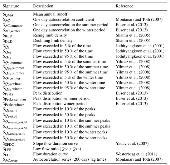
Table 3.Overview of the hydrological signatures.
Signature Description Reference
SQMA Mean annual runoff
SAC One day autocorrelation coefficient Montanari and Toth (2007) SAC,summer One day autocorrelation the summer period Euser et al. (2013) SAC,winter One day autocorrelation the winter period Euser et al. (2013)
SRLD Rising limb density Shamir et al. (2005)
SDLD Declining limb density Shamir et al. (2005)
SQ5 Flow exceeded in 5 % of the time Jothityangkoon et al. (2001)
SQ50 Flow exceeded in 50 % of the time Jothityangkoon et al. (2001)
SQ95 Flow exceeded in 95 % of the time Jothityangkoon et al. (2001)
SQ5,summer Flow exceeded in 5 % of the summer time Yilmaz et al. (2008)
SQ50,summer Flow exceeded in 50 % of the summer time Yilmaz et al. (2008)
SQ95,summer Flow exceeded in 95 % of the summer time Yilmaz et al. (2008)
SQ5,winter Flow exceeded in 5 % of the winter time Yilmaz et al. (2008)
SQ50,winter Flow exceeded in 50 % of the winter time Yilmaz et al. (2008)
SQ95,winter Flow exceeded in 95 % of the winter time Yilmaz et al. (2008)
SPeaks Peak distribution Euser et al. (2013)
SPeaks,summer Peak distribution summer period Euser et al. (2013) SPeaks,winter Peak distribution winter period Euser et al. (2013) SQpeak,10 Flow exceeded in 10 % of the peaks
SQpeak,50 Flow exceeded in 50 % of the peaks SQsummer,peak,10 Flow exceeded in 10 % of the summer peaks SQsummer,peak,50 Flow exceeded in 10 % of the summer peaks SQwinter,peak,10 Flow exceeded in 10 % of the winter peaks
SQwinter,peak,50 Flow exceeded in 50 % of the winter peaks
SSFDC Slope flow duration curve Yadav et al. (2007) SLFR Low flow ratio (Q90/ Q50)
SFDC Flow duration curve Westerberg et al. (2011)
SAC,serie Autocorrelation series (200 days lag time) Montanari and Toth (2007)
at any timet+1 are less dependent on the flows att, which points towards less memory and thus less storage in the sys-tem (i.e. reducedSR), leading to increased peak flows,
simi-lar to the reports of, for example, Patric and Reinhart (1971) for one of the Fernow experiments.
The declining limb density for HJ Andrews WS1 (Fig. 2g) shows increased values right after deforestation, whereas a longer time after deforestation, the values seem to plot closer to the values obtained from the reference watershed. This indicates that for the same number of peaks, less time was needed for the recession in the hydrograph in the early years after logging. In contrast, the rising limb density shows in-creased values during and right after deforestation for Hub-bard Brook WS2 and WS5 (Fig. 2k–l), compared to the ref-erence watershed. Here, less time was needed for the rising part of the hydrograph in the more early years after logging. Thus, the recession seems to be affected in HJ Andrews WS1, whereas the Hubbard Brook watersheds exhibit a quicker rise of the hydrograph.
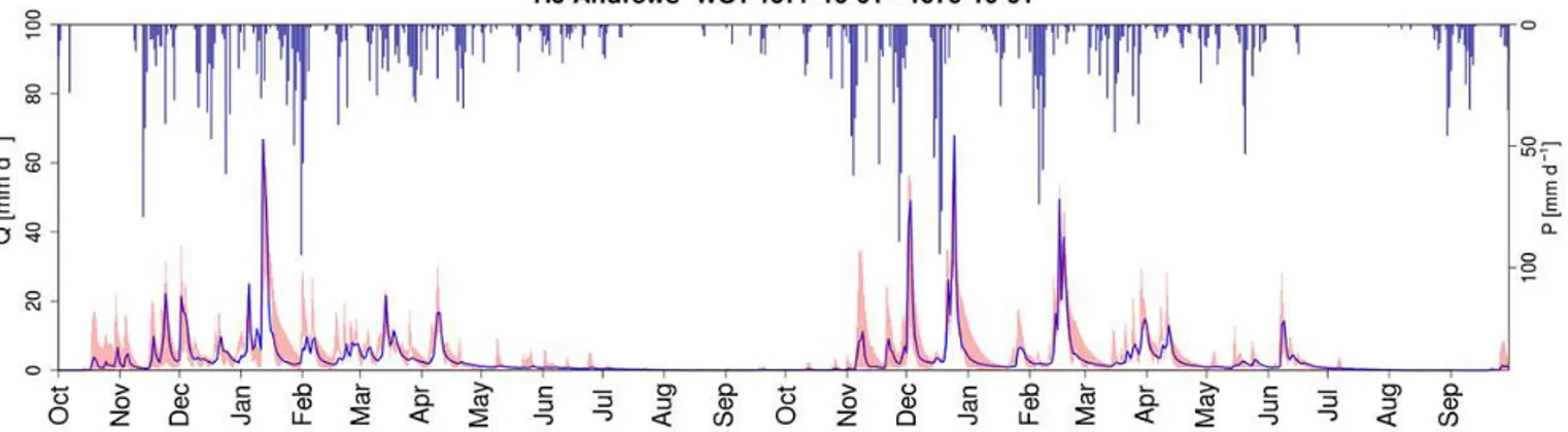
Eventually, the flow duration curves, as shown in Fig. 2m– o, indicate a higher variability of flows, as the years follow-ing deforestation plot with an increased steepness of the flow duration curve, i.e. a higher flashiness. This increased
flashi-ness of the catchments after deforestation can also be noted from the hydrographs shown in Fig. 3. The peaks in the hy-drographs are generally higher, and the flows return faster to the baseflow values in the years right after deforestation than some years later after some forest regrowth, all with simi-lar values for the yearly sums of precipitation and potential evaporation.
4.2 Temporal evolution ofSRandSu,max
The observed changes in the hydrological response of the study catchments (as discussed above) were also clearly re-flected in the temporal evolution of the root-zone storage ca-pacities as described by the catchment models (Fig. 4). The models all exhibited Kling–Gupta efficiencies ranging be-tween 0.5 and 0.8 and Kling–Gupta efficiencies of the log of the flows between 0.2 and 0.8 (see the Supplement Figs. S5– S7, with all posterior parameter distributions in Figs. S10– S27, and the number of feasible solutions in Tables S5– S7 in the Supplement). Comparing the water-balance- and model-derived estimates of root-zone storage capacity SR
andSu,max, respectively, then showed that they exhibit very
Figure 3. Hydrographs for HJ Andrews WS1 in (a) 1962 (annual precipitation PA=2018, Ep,A=951 mm yr−1) and (b) 1989 (PA=1752,Ep,A=846 mm yr−1), Hubbard Brook WS2 in(c)1966 (PA=1222,Ep,A=788 mm yr−1and(d) 2004 (PA=1296, an-nual Ep,A=761 mm yr−1 and Hubbard Brook WS5 in(e)1984 (PA=1480, annualEp,A=721 mm yr−1) and(f) 2004 (PA=1311, Ep,A=731 mm yr−1).
Andrews WS1 and Hubbard Brook WS2, root-zone storage capacities sharply decreased after deforestation and gradu-ally recovered during regrowth towards a dynamic equilib-rium of climate and vegetation, whereas the undisturbed ref-erence catchments of HJ Andrews WS2 and Hubbard Brook WS3 showed a rather constant signal over the full period (see Fig. S8).
The HJ Andrews WS1 shows the clearest signal when looking at the water-balance-derived SR, as can be seen by
the green shaded area in Fig. 4a. Before deforestation, the root-zone storage capacity SR,1yr was found to be around
400 mm. During deforestation, theSR,1yrrequired to provide
the remaining vegetation with sufficient and continuous ac-cess to water decreased from around 400 to 200 mm. For the first 4–6 years after deforestation theSR,1yrincreased again,
reflecting the increased water demand of vegetation with the regrowth of the forest. In addition, it was observed that in the period 1971–1978 SR,1yr slowly decreased again in HJ
Andrews.
The four models show a similar pronounced decrease of the calibrated, feasible set ofSu,maxduring deforestation and
a subsequent gradual increase over the first years after de-forestation. The model concepts, and thus our assumptions about nature, can therefore only account for the changes in hydrological response dynamics of a catchment, when cali-brated in a window calibration approach with different pa-rameterizations for each time frame. The absolute values of Su,maxobtained from the most parsimonious HYMOD and
FLEX models (both with 8 free calibration parameters) show a somewhat higher similarity toSR,1yrand its temporal
evo-lution than the values from the other two models. In spite of similar general patterns inSu,max, the higher number of
pa-rameters in TUW (i.e. 15) result, due to compensation effects between individual parameters, in wider uncertainty bounds which are less sensitive to change. It was also observed that in particular TUW overestimatesSu,maxcompared toSR,1yr,
which can be attributed to the absence of an interception reservoir, leading to a root zone that has to satisfy not only transpiration but all evaporative fluxes.
Hubbard Brook WS2 exhibits a similarly clear decrease in root-zone storage capacity as a response to deforestation, as shown in Fig. 4b. The water-balance-basedSR,1yrestimates
approach values of zero during and right after deforestation. In these years the catchment was treated with herbicides, re-moving effectively any vegetation, thereby minimizing tran-spiration. In this catchment a more gradual regrowth pattern occurred, which continued after logging started in 1966 until around 1983.
Generally, the models applied in Hubbard Brook WS2 show similar behaviour to those in the HJ Andrews catch-ment. The calibratedSu,maxclearly follows the temporal
pat-tern ofSR,1yr, reflecting the pronounced effects of de- and
reforestation. It can, however, also be observed that the ab-solute values ofSu,max exceed the SR,1yr estimates. While
FLEX on balance exhibits the closest resemblance between the two values, the TUW model in particular exhibits wide uncertainty bounds with elevatedSu,maxvalues. Besides the
re-Figure 4.Evolution of root-zone storage capacitySR,1yrfrom water balance-based estimation (green shaded area, a range of solutions due to the sampling of the unknown interception capacity) compared withSu,max,2yrestimates obtained from the calibration of four models (FLEX, HYPE, TUW, HYMOD; blue box plots) for HJ Andrews WS1, Hubbard Brook WS2 and Hubbard Brook WS5. Red shaded areas are periods of deforestation.
duces the importance of the model parameter Su,max, and
makes it thereby more difficult to identify by calibration. The parameter is most important for lengthy dry periods when vegetation needs enough storage to ensure continuous access to water.
The temporal variation inSRin Hubbard Brook WS5 does
not show such a distinct signal as in the other two study catchments (Fig. 4c). Moreover, it can be noted that in the summers of 1984 and 1985 the values ofSR,1yrare relatively
high. Nevertheless, the model-based values ofSu,max show
val-Figure 5.Observed and modelled hydrograph for HJ Andrews WS1 for the years of 1978 and 1979, with the red coloured area indicating the 5/95 % uncertainty intervals of the modelled discharge. Blue bars show daily precipitation.
ues. TUW and HYMOD show again higher model-based val-ues, but FLEX is also now overestimating the root-zone stor-age capacity.
4.3 Process understanding – trend analysis and change in hydrological regimes
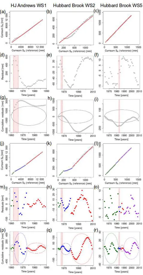
The trend analysis for water-balance-derived values ofSR,1yr
suggests that for all three study catchments significantly dif-ferent hydrological regimes in time can be identified before and after deforestation, linked to changes inSR,1yr(Fig. 7).
For all three catchments, the cumulative residuals plot out-side the 95 %-confidence ellipse, indicating that the time se-ries obtained in the control catchments and the deforested catchments are not homogeneous (Fig. 7g–i).
Rather obvious break points can be identified in the resid-uals plots for the catchments HJ Andrews WS1 and Hubbard Brook WS2 (Fig. 7d–e). Splitting up the SR,1yr time series
according to these break points into the periods before de-forestation, deforestation and recovery resulted in three indi-vidually homogenous time series that are significantly differ-ent from each other, indicating switches in the hydrological regimes. The results shown in Fig. 4 indicate that these catch-ments developed a rather stable root-zone storage capacity sometime after the start of deforestation (for HJ Andrews WS1 after 1964, for Hubbard Brook WS2 after 1967). Hence, recovery and deforestation balanced each other, leading to a temporary equilibrium. The recovery signal then becomes more dominant in the years after deforestation. The third ho-mogenous period suggests that the root-zone storage capacity reached a dynamic equilibrium without any further system-atic changes. This can be interpreted in the way that in the HJ Andrews WS1, hydrological recovery after deforestation due to the recovery of the root-zone storage capacity took about 6–9 years (Fig. 7p), while Hubbard Brook WS2 required 10– 13 years for hydrological recovery (Fig. 7q). This strongly supports the results of Hornbeck et al. (2014), who reported
changes in water yield for WS2 for up to 12 years after de-forestation.
The identification of different periods is less obvious for Hubbard Brook WS5, but the two time series of control catchment and treated catchment are significantly different (see the cumulative residuals in Fig. 7i). Nevertheless, the most obvious break point in residuals can be found in 1989 (Fig. 7f). In addition, it can be noted that turning points also exist in 1983 and 1985. These years can be used to split the time series into four groups (leading to the periods of 1964–1982, 1983–1985, 1986–1989 and 1990–2009 for fur-ther analysis). The cumulative residuals from the new re-gressions, based on the grouping, plot within the confidence bounds again, and show a period with deforestation (1983– 1985) and recovery (1986–1989). Mou et al. (1993) reported similar findings with the highest biomass accumulation in 1986 and 1988, and slower vegetation growth in the early years. Therefore, full recovery took 5–6 years in Hubbard Brook WS5.
4.4 Time-variant model formulation
The adjusted model routine for FLEX, which uses a dynamic time series of Su,max, generated with the Weibull growth
function (Eq. 12), resulted in a rather small impact on the overall model performance in terms of the calibration ob-jective function values (Fig. 8b, d, f) compared to the time-invariant formulation of the model. The strongest improve-ments for calibration were observed for the dynamic formu-lation of FLEX for HJ Andrews WS1 and Hubbard Brook WS2 (Fig. 8b and d), which reflects the rather clear signal from deforestation in these catchments.
Evaluating a set of hydrological signatures suggests that the dynamic formulation ofSu,maxallows the model to have
Figure 6.Observed and modelled hydrograph for Hubbard Brook WS2 for(a)the years of 1984 and 1985 and(b)the years of 1986 and 1987, with the red coloured area indicating the 5/95 % uncertainty intervals of the modelled discharge. Blue bars show daily precipitation.
the cases improvements are observed. Most signatures for HJ Andrews WS1 show a high probability of improvement, with a maximum PI,S=0.69 (for SQ95,wint er)and an
aver-age PI,S=0.55. Considering the large difference between the deforested situation and the new equilibrium situation of about 200 mm, this supports the hypothesis that here a time-variant formulation of Su,max does provide means for
an improved process representation and, thus, hydrologi-cal signatures. Here, improvements are observed especially in the high flows in summer (SQ5,summer, SQ50,summer)and
peak flows (e.g.SPeaks,SPeaks,summer,SPeaks,winter), which
il-lustrates that the root-zone storage affects mostly the fast-responding components of the system.
At Hubbard Brook WS2 a more variable pattern is shown in the ability of the model to reproduce the hydrological sig-natures. It is interesting to note that the low flows (SQ95,
SQ95,summer,SQ50,summer)improve, opposed to the
expecta-tion raised by the argumentaexpecta-tion for HJ Andrews WS1 that peak flows and high flows should improve. In this case, the peaks are too high for the time-dynamic model.
The probabilities of improvement for the signatures in Hubbard Brook WS5 show an even less clear signal: the model cannot clearly identify a preference for either a dynamic or static formulation of Su,max (relatively white
colours in Fig. 9). This absence of a clear preference can be
related to the observed patterns in water-balance-derivedSR
(Fig. 4c), which also does not show a very clear signal after deforestation, indicating that the root-zone storage capacity is of less importance in this humid region characterized by limited seasonality.
5 Discussion
5.1 Deforestation and changes in hydrological response dynamics
The changes found in the runoff behaviour of the deforested catchments point towards shifts in the yearly sums of transpi-ration, which can, except for climatic variation, be linked to the regrowth of vegetation that takes place at a similar pace to the changes in hydrological dynamics. This coincidence of regrowth dynamics and evolution of runoff coefficients was not only noticed by Hornbeck et al. (2014) for the Hubbard Brook, but was also previously acknowledged for example by Swift and Swank (1981) in the Coweeta experiment or Kuczera (1987) for eucalypt regrowth after forest fires.
Figure 8.The time invariantSu,maxformulation represented bySR,20yr(yellow) and time dynamicSu,maxfitted Weibull growth function (blue) with a linear reduction during deforestation (red shaded area) and mean 20-year return period root-zone storage capacitySR, 20yras equilibrium value for(a)HJ Andrews WS1 witha=0.0001 days−1,b=1.3 andSR,20yr=494 mm with(b)the objective function values,
Figure 9.Signature comparison between a time-dynamic and time-invariant formulation of root-zone storage capacity in the FLEX model with (a)probabilities of improvement and(b) Ranked Probability Score for 28 hydrological signatures for HJ Andrews WS1 (HJA1), Hubbard Brook WS2 (HB2) and Hubbard Brook WS5 (HB5). High values are shown in blue, whereas a low values are shown in red.
tion is removed. Similarly, Gao et al. (2014) found a strong correlation between root-zone storage capacities and runoff coefficients in more than 300 US catchments, which lends further support to the hypothesis that root-zone storage ca-pacities may have decreased in deforested catchments right after removal of the vegetation.
5.2 Temporal evolution ofSRandSu,max
The differences between the Hubbard Brook catchments and HJ Andrews catchments can be related to climatic conditions. In spite of the high annual precipitation volumes, highSR,1yr
(Köppen–Geiger class Csb) and the approximately 6-month phase shift between precipitation and potential evaporation peaks in the study catchment, which dictates that the stor-age capacities need to be large enough to store precipitation, which falls mostly during winter, throughout the extended dry periods with higher energy supply throughout the rest of the year (Gao et al., 2014). At the same time, lowSR,1yr
val-ues in Hubbard Brook WS2 can be related to the relatively humid climate, and the absence of pronounced rainfall sea-sonality strongly reduces storage requirements.
It can also be argued that there is a strong influence of the inter-annual climatic variability on the estimated root-zone storage capacities. For example, the marked increase in SR,1yrin Hubbard Brook WS2 in 1985 rather points
to-wards an exceptional year, in terms of climatological fac-tors, than a sudden expansion of the root zone. It can also be observed from Fig. 3a that the runoff coefficient was rela-tively low for 1985, suggesting either increased evaporation or a storage change. A combination of a relatively long pe-riod of low rainfall amounts and high potential evaporation, as can be noted by the relatively high mean annual poten-tial evaporation on top of Fig. 4b, may have led to a high demand in 1985. Parts of the vegetation may not have sur-vived these high-demand conditions due to insufficient ac-cess to water, explaining the dip inSR,1yr for the following
year, which is also in agreement with reduced growth rates of trees after droughts as observed by for example Bréda et al. (2006). The hydrographs of 1984–1985 (Fig. 6a) and 1986–1987 (Fig. 6b) also show that July–August 1985 was exceptionally dry, whereas the next year in August 1986 the catchment seems to have increased peak flows. This either points towards an actual low storage capacity due to contrac-tion of the roots during the dry summer or a low need of the system to use the existing capacity, for instance to recover other vital aspects of the system.
Nevertheless, Hubbard Brook WS2 does not show a clear signal of reduced root-zone storage, followed by a gradual regrowth. Here, the forest was removed in a whole-tree har-vest in winter 1983–1984, followed by natural regrowth. The summers of 1984 and 1985 were very dry summers, as also reflected by the high values ofSR,1yr. The young system had
already developed enough roots before these dry periods to have access to a sufficiently large water volume to survive this summer. This is plausible, as the period of the highest deficit occurred in mid-July and lasted until approximately the end of September, thus long after the beginning of the growing season, allowing enough time for an initial growth and development of young roots from April until mid-July. In addition, the composition of the new forest differed from the old forest, with more pin cherry (Prunus pensylvanica) and paper birch (Betula papyrifera). This supports the statements of a quick regeneration as these species have a high growth rate and reach canopy closure in a few years. Furthermore, the forest was not either treated with herbicides (Hubbard Brook WS2) or burned (HJ Andrews WS1), leaving enough
low shrubs and herbs to maintain some level of transpira-tion (Hughes and Fahey, 1991; Martin, 1988). It can thus be argued, similar to Li et al. (2007), that the remaining vege-tation experienced less competition and could increase root water uptake efficiency and transpiration per unit leaf area. This is in agreement with Hughes and Fahey (1991), who also stated that several species benefited from the removal of canopies and newly available resources in this catchment. Lastly, several other authors related the absence of a clear change in hydrological dynamics to the severe soil distur-bance in this catchment (Hornbeck et al., 1997; Johnson et al., 1991). These disturbances lead to extra compaction, whereas at the same time species were changing, effectively masking any changes in runoff dynamics.
5.3 Process understanding – trend analysis and change in hydrological regimes
The found recovery periods correspond to recovery timescales for forest systems as reported in other studies (e.g. Brown et al., 2005; Hornbeck et al., 2014; Elliott et al., 2016) which found that catchments reach a new equilibrium with a similar timescale as reported here, but in this case with the direct link to the parameter describing the catchment-scale root-zone storage capacity. The timescales are also in agree-ment with regression models to predict water yield after log-ging of Douglass (1983), who assumed a duration of water yield increases of 12 years for coniferous catchments.
The timescales found here are around 10 years (5–13 years for the catchments under consideration), but will probably depend on climatic factors and vegetation type. HJ Andrews WS1 has a recovery (6–9 years) slightly shorter compared to Hubbard Brook WS2 (10–13 years), which could depend on the different climatological conditions of the catchments. Nevertheless, it could also be argued that the spraying of her-bicides had an especially strong impact on the recovery of vegetation in Hubbard Brook WS2, as the Hubbard Brook WS5 does not show such a distinct recovery signal.
5.4 Time-variant model formulation
It was found that a time-dynamic formulation of Su,max
Figure 10.Hydrograph of Hubbard Brook WS2 with the observed discharge (blue) and the modelled discharge represented by the 5/95 % uncertainty intervals (red), obtained with(a)a constant representation of the root-zone storage capacitySu,max and(b) a time-varying representation of the root-zone storage capacitySu,max. Blue bars indicate precipitation.
Nevertheless, signatures considering the peak flows did not improve for the Hubbard Brook catchments. Apparently, the model with a constant, and thus higher,Su,maxstored
wa-ter in the root zone, reducing recharge to the groundwawa-ter reservoir that maintains the lower flows and buffering more water, reducing the peaks. This can also be clearly seen from the hydrographs (Fig. 10), where the later part of the re-cession in the late-summer months is much better captured by the time-dynamic model. Nevertheless, the peaks are too high for the time-dynamic model, which here is linked to an insufficient representation of snow-related processes, as can be seen from the hydrograph (April–May) as well, and possi-bly by an inadequate interception growth function, both lead-ing to too high amounts of effective precipitation enterlead-ing the root zone. An adjustment of these processes would have resulted in less infiltration and a smaller root-zone storage capacity.
It was acknowledged previously by several authors that certain model parameters may need time-dynamic tions, like Waichler et al. (2005) with time-dynamic formula-tions of leaf area index and overstore height for the DHSVM model. In addition, Westra et al. (2014) captured long-term dynamics in the storage parameter of the GR4J model with a trend correction, in fact leading to a similar model behaviour to the Weibull growth function in this study. Nevertheless,
they only hypothesized about the actual hydrological reasons for this, which aimed at the changing number of farmer dams in the catchment. The results presented here indicate that vegetation, and especially root-zone dynamics, has a strong impact on the long term non-stationarity of model parame-ters. The simple Weibull equation can be used as an extra equation in conceptual hydrological models to more closely reflect the dynamics of vegetation. The additional growth pa-rameters may be left for calibration, but can also be esti-mated from simple water-balance-based estimations of the root-zone storage. In this way, the extra parameters should not add any uncertainty to the model outcomes.
5.5 General limitations
The results presented here depend on the quality of the data and several assumptions made in the calculations. A limiting factor is that the potential evaporation is determined from temperature only, leading to values that may be relatively low and water balances that may not close completely. Gen-erally, this would lead to a discrepancy between the mod-elledSu,max, where potential evaporation is directly used, and
the water-balance estimates ofSR. The models will probably
the rather low potential evaporation. This can also be noted when looking at Fig. 4 for several models.
In addition, the assumption that the water balance closes in the 2-year periods under consideration may often be violated in reality. It can be argued that the estimated transpiration for the calculation ofSRrepresents an upper boundary, when
storage changes are ignored. This would lead to estimates of SRthat may be lower than presented here. Nevertheless,
attempts with 5-year water balances to reduce the influence of storage changes (see Fig. S9), showed that similar patterns were obtained. Values here were slightly lower due to more averaging in the estimation of the transpiration by the longer time period used for the water balance. Nevertheless, a strong decrease after deforestation and gradual recovery can still be observed.
The issues raised here can be fully avoided when, instead of a water-balance-based estimation of the transpiration, re-mote sensing products are used to estimate the transpiration, similar to Wang-Erlandsson et al. (2016). However, water-balance-based estimates may provide a rather quick solution. The transpiration estimates were also only corrected for interception evaporation, thus assuming a negligible amount of soil evaporation. Making this additional separation is typ-ically not warranted by the available data and would result in additional uncertainty. The transpiration estimates presented here merely represent an upper limit of transpiration and will be lower in reality due to soil evaporation. Thus, the values forSR,1yrmay expected to be lower in reality as well.
6 Conclusions
In this study, three deforested catchments (HJ Andrews WS1, Hubbard Brook WS2 and WS5) were investigated to assess the dynamic character of root-zone storage capacities us-ing water balance, trend analysis, four different hydrologi-cal models and one modified model version. Root-zone stor-age capacities were estimated based on a simple water bal-ance approach. Results demonstrate a good correspondence between water-balance-derived root-zone storage capacities and values obtained by a 2-year moving window calibration of four distinct hydrological models.
There are significant changes in root-zone storage capac-ity after deforestation, which were detected by both a water-balance-based method and the calibration of hydrological models in two of the three catchments. More specifically, root-zone storage capacities showed, for HJ Andrews WS1 and Hubbard Brook WS2, a sharp decrease in root-zone stor-age capacities immediately after deforestation with a grad-ual recovery towards a new equilibrium. This could to a large extent explain post-treatment changes to the hydrologi-cal regime. These signals were however not clearly observed for Hubbard Brook WS5, probably due to soil disturbance, a new vegetation composition and a climatologically excep-tional year. Nevertheless, trend analysis showed significant
differences for all three catchments with their correspond-ing, undisturbed reference watersheds. Based on this, recov-ery times were estimated to be between 5 and 13 years for the three catchments under consideration.
These findings underline the fact that root-zone storage ca-pacities in hydrological models, which are more often than not treated as constant in time, may need time-dynamic for-mulations with reductions after logging and gradual regrowth afterwards. Therefore, one of the models was subsequently formulated with a time-dynamic description of root-zone storage capacity. Particularly under climatic conditions with pronounced seasonality and phase shifts between precipita-tion and evaporaprecipita-tion, this resulted in improvements in model performance as evaluated by 28 hydrological signatures.
Even though this more complex system behaviour may lead to extra unknown growth parameters, it has been shown here that a simple equation, reflecting the long-term growth of the system, can already suffice for a time-dynamic es-timation of this crucial hydrological parameter. Therefore, this study clearly shows that observed changes in runoff characteristics after land-cover changes can be linked to relatively simple time-dynamic formulations of vegetation-related model parameters.
7 Data availability
The Supplement related to this article is available online at doi:10.5194/hess-20-4775-2016-supplement.
Acknowledgements. We would like to acknowledge the European Commission FP7 funded research project “Sharing Water-related Information to Tackle Changes in the Hydrosphere – for Opera-tional Needs” (SWITCH-ON, grant agreement number 603587), as this study was conducted within the context of SWITCH-ON as an example of scientific potential when using open data for collabora-tive research in hydrology.
Open Data were provided by the Hubbard Brook Ecosystem Study (HBES), which is a collaborative effort at the Hubbard Brook Experimental Forest which is operated and maintained by the USDA Forest Service Northern Research Station, Newtown Square, PA, USA.
Open Data were provided by the HJ Andrews Experimental Forest research program, funded by the National Science Founda-tion’s Long-Term Ecological Research Program (DEB 08-23380), US Forest Service Pacific Northwest Research Station, and Oregon State University.
Edited by: F. Fenicia
Reviewed by: A. Ducharne and two anonymous referees
References
Alila, Y., Kura´s, P. K., Schnorbus, M., and Hudson, R.: Forests and floods: A new paradigm sheds light on age-old controversies, Water Resour. Res., 45, W08416, doi:10.1029/2008WR007207, 2009.
Allen, C. D., Macalady, A. K., Chenchouni, H., Bachelet, D., Mc-Dowell, N., Vennetier, M., Kitzberger, T., Rigling, A., Bres-hears, D. D., Hogg, E. H., Gonzalez, P., Fensham, R., Zhang, Z., Castro, J., Demidova, N., Lim, J.-H., Allard, G., Run-ning, S. W., Semerci, A., and Cobb, N.: A global overview of drought and heat-induced tree mortality reveals emerging climate change risks for forests, Forest Ecol. Manage., 259, 660–684, doi:0.1016/j.foreco.2009.09.001, 2010.
Allen, R. G., Pereira, L. S., Raes, D., and Smith, M.: Crop evapotranspiration-Guidelines for computing crop water requirements-FAO Irrigation and drainage paper 56, FAO, Rome, 300, D05109, 1998.
Allison, G. B., Cook, P. G., Barnett, S. R., Walker, G. R., Jolly, I. D., and Hughes, M. W.: Land clearance and river salinisation in the western Murray Basin, Australia, J. Hydrol., 119, 1–20, doi:10.1016/0022-1694(90)90030-2, 1990.
Andersson, L. and Arheimer, B.: Consequences of changed wet-ness on riverine nitrogen – human impact on retention vs. natural climatic variability, Reg. Environ. Change, 2, 93–105, doi:10.1007/s101130100024, 2001.
Andréassian, V.: Waters and forests: from historical con-troversy to scientific debate, J. Hydrol., 291, 1–27, doi:10.1016/j.jhydrol.2003.12.015, 2004.
Bathurst, J. C., Ewen, J., Parkin, G., O’Connell, P. E., and Cooper, J. D.: Validation of catchment models for
predict-ing land-use and climate change impacts, 3. Blind valida-tion for internal and outlet responses, J. Hydrol., 287, 74–94, doi:10.1016/j.jhydrol.2003.09.021, 2004.
Bergström, S.: Development and application of a conceptual runoff model for Scandinavian catchments, SMHI Reports RHO, Nor-rköping, 1976.
Bergström, S.: The HBV model: Its structure and applications, Swedish Meteorological and Hydrological Institute, 1992. Black, P. E.: Watershed functions1, JAWRA Journal of the
Ameri-can Water Resources Association, 33, 1–11, doi:10.1111/j.1752-1688.1997.tb04077.x, 1997.
Bosch, J. M. and Hewlett, J. D.: A review of catchment experiments to determine the effect of vegetation changes on water yield and evapotranspiration, J. Hydrol., 55, 3–23, doi:10.1016/0022-1694(82)90117-2, 1982.
Boyle, D. P.: Multicriteria calibration of hydrologic models, 2001. Brath, A., Montanari, A., and Moretti, G.: Assessing the
ef-fect on flood frequency of land use change via hydrologi-cal simulation (with uncertainty), J. Hydrol., 324, 141–153, doi:10.1016/j.jhydrol.2005.10.001, 2006.
Bréda, N., Huc, R., Granier, A., and Dreyer, E.: Temperate forest trees and stands under severe drought: a review of ecophysiologi-cal responses, adaptation processes and long-term consequences, Ann. Forest Sci., 63, 625–644, 2006.
Breuer, L., Eckhardt, K., and Frede, H.-G.: Plant parameter values for models in temperate climates, Ecol. Modell., 169, 237–293, doi:10.1016/S0304-3800(03)00274-6, 2003.
Brown, A. E., Zhang, L., McMahon, T. A., Western, A. W., and Vertessy, R. A.: A review of paired catch-ment studies for determining changes in water yield result-ing from alterations in vegetation, J. Hydrol., 310, 28–61, doi:10.1016/j.jhydrol.2004.12.010, 2005.
Brunner, I., Herzog, C., Dawes, M. A., Arend, M., and Sperisen, C.: How tree roots respond to drought, Front. Plant Sci., 6, 547, doi:10.3389/fpls.2015.00547, 2015.
Brunner, P. and Simmons, C. T.: HydroGeoSphere: A Fully Inte-grated, Physically Based Hydrological Model, Ground Water, 50, 170–176, doi:10.1111/j.1745-6584.2011.00882.x, 2012. Campbell, J.: Hubbard Brook Experimental Forest (USDA
For-est Service): Daily Streamflow by Watershed, 1956–present, available at: http://www.hubbardbrook.org/data/dataset.php?id= 2 (last access: 29 November 2016), 2014a.
Campbell, J.: Hubbard Brook Experimental Forest (US Forest Ser-vice): Daily Precipitation Standard Rain Gage Measurements, 1956–present, available at: http://www.hubbardbrook.org/data/ dataset.php?id=13 (last access: 29 November 2016), 2014b. Campbell, J.: Hubbard Brook Experimental Forest (USDA Forest
Service): Daily Maximum and Minimum Temperature Records, 1955–present, available at: http://www.hubbardbrook.org/data/ dataset.php?id=59, 2014c.
Campbell, J.: Hubbard Brook Experimental Forest (USDA For-est Service): Daily Mean Temperature Data, 1955–present, available at: http://www.hubbardbrook.org/data/dataset.php?id= 58, 2014d.