www.hydrol-earth-syst-sci.net/13/1375/2009/ © Author(s) 2009. This work is distributed under the Creative Commons Attribution 3.0 License.
Earth System
Sciences
Temporal variation of soil moisture over the Wuding River basin
assessed with an eco-hydrological model, in-situ observations and
remote sensing
S. Liu1, X. Mo1, W. Zhao2, V. Naeimi3, D. Dai2, C. Shu1, and L. Mao4
1Key Laboratory of Water Cycle & Related Land Surface Processes, Institute of Geographic Sciences & Natural Resources
Research, Chinese Academy of Sciences, Beijing, 100101, China
2The Bureau of Hydrology, Yellow River Conservancy Committee, Zhengzhou, 450004, China
3Institute of Photogrammetry and Remote Sensing, Vienna University of Technology, Gusshausstrasse 27–29,
1040 Vienna, Austria
4China Meteorology Administration, National Meteorological Center, Beijing, 100081, China
Received: 7 October 2008 – Published in Hydrol. Earth Syst. Sci. Discuss.: 6 December 2008 Revised: 5 May 2009 – Accepted: 19 May 2009 – Published: 31 July 2009
Abstract. The change pattern and trend of soil moisture (SM) in the Wuding River basin, Loess Plateau, China is ex-plored based on the simulated long-term SM data from 1956 to 2004 using an eco-hydrological process-based model, Vegetation Interface Processes model, VIP. In-situ SM obser-vations together with a remotely sensed SM dataset retrieved by the Vienna University of Technology are used to vali-date the model. In the VIP model, climate-eco-hydrological (CEH) variables such as precipitation, air temperature and runoff observations and also simulated evapotranspiration (ET), leaf area index (LAI), and vegetation production are
used to analyze the soil moisture evolution mechanism. The results show that the model is able to capture seasonal SM variations. The seasonal pattern, multi-year variation, stan-dard deviation and coefficient of variation (CV) of SM at the
daily, monthly and annual scale are well explained by CEH variables. The annual and inter-annual variability of SM is the lowest compared with that of other CEH variables. The trend analysis shows that SM is in decreasing tendency at α=0.01 level of significance, confirming the Northern Dry-ing phenomenon. This trend can be well explained by the decreasing tendency of precipitation (α=0.1) and increasing tendency of temperature (α=0.01). The decreasing tendency of runoff has higher significance level (α=0.001). Because of SM’s decreasing tendency, soil evaporation (ES) is also
Correspondence to:S. Liu ([email protected])
decreasing (α=0.05). The tendency of net radiation (Rn),
evapotranspiration (ET), transpiration (EC), canopy
inter-cept (EI) is not obvious. Net primary productivity (NPP), of
which the significance level is lower thanα=0.1, and gross primary productivity (GPP) atα=0.01 are in increasing ten-dency.
1 Introduction
The Wuding River basin, in the Loess Plateau, China has been suffered severe soil erosion damages. Understanding long-term change of soil moisture (SM) in the basin, located in a transition zone from farmland and grassland to desert in the Plateau, is very important as it provides useful infor-mation for making scientific suggestions for early warning of land desertification, ecosystem recovery and also efficient soil and water management.
Unfortunately, all over the world, including the study basin, long-term SM data are very scarce. Hence, the models and remote sensing technique are used to extend the SM data both in space and time.
Physically process-based models are thus used to ob-tain reliable prediction of long-term SM. So far several SM datasets have been produced using different land surface pro-cess models. However most of the models have simple SM schemes (e.g., Liu et al., 2003) or are forced with monthly average, which made the simulated SM results not agree well with the observations (Chen et al., 1997; Entin et al., 1999; Schlosser et al., 2000). Soil moisture is an important ele-ment in hydrological cycle which is closely related to wa-ter and energy transfer between soil, vegetation, and atmo-sphere. It has been shown that much of the global warming so far was at night (Karl et al., 1991, 1993; Folland et al., 1992; Stenchikov and Robock, 1995; Robock et al., 2000). So at least models with diurnal cycle are needed to correctly simulate SM. The SM may also be characterized by auto-correlation in time, which means that the lagged effects in inputs or losses can be important as much as those occurring at the time that the impacts are actually observed (Hamlet et al., 2007). A physically process-based model with detailed information about soil-vegetation-atmosphere water and en-ergy transfer is needed to correctly simulate long term SM time series for trend analysis.
There are at least three prevailing methods to do the trend analysis. The first is to draw the linearly regressive trend line over the time series of data to see if it is in upward (increas-ing) or downward (decreas(increas-ing) trend (Robock et al., 2000). The second is performing the nonparametric Mann-Kendall (M-K) trend test (Mann, 1945; Kendall, 1975; Hirsch and Slack, 1984; Gilbert, 1987) and judging the trend by the value of the M-K statistic (e.g., Sheffield and Wood, 2008). The last not the least is to compare the SM averaged among each of the decades, which is broadly used in the related studies in China (e.g., Yan et al., 1999). Within the long-term trends, there are noticeable inter-annual and decadal variations in SM for most regions, which weaken the robust-ness of the trends and have to be considered in trend studies (Sheffield and Wood, 2008).
The M-K trend test has received the greatest attention in hydrology due to its free-distribution nature, which makes it more suitable than parametric alternatives for testing hydro-logical data. However, the use of M-K trend test is limited to the assumption that the data must be independent and iden-tically distributed (IID). One of the solutions to overcome the problem is transforming the real data into a time series, in which its autocorrelation coefficient is zero. Zero auto-correlation coefficient indicates that the data are independent and identically distributed. So the solution turns to be how to make data series with non-zero autocorrelation coefficient into data series with autocorrelation coefficient being zero. One of such solutions is called “prewhitening” (von Storch, 1995) – von Storch method. It is assumed that data seriesxi
with a non-zero autocorrelation coefficient can be modelled by an autoregressive first order model (Box et al., 1994):
yi =xi−ρ1xi−1, (1)
whereρ1 is the lag-1 autocorrelation coefficient (Kulkarni
and von Storch, 1995; Douglas et al., 2000; Zhang et al., 2001). However, it is found that the trend computed from such a prewhitened time series is smaller, since the trend in the prewhitened data has a slope (Wang and Swail, 2001) as
µpw=(1−ρ1)µ (2)
whereµpw andµare the trend for the prewhitened and the
original data respectively.
At least two methods are proposed to avoid this prob-lem. One of them is using the iterative procedure proposed by Zhang et al. (2000), refined by Wang and Swail (2001) and Zhang and Zwiers (2003). In this method, called Zhang method, the autocorrelation is computed after removing the significant trends from the series. This process is continued until the differences in the estimates of the slope and theρ1
in two consecutive iterations become negligible. The M-K test for trend is run on the resulted time series and then Sen approach (Sen, 1968) is used to compute the slope.
Another method is Trend Free Pre-whitening procedure proposed by Yue and Pilon (Yue et al., 2002) – called Yue method. In this method, the slope of a trend in sample data is estimated using the approach proposed by Sen (1968). As-suming the trend is linear, the sample data are detrended by subtracting the trend from the sample data. The lag-1 se-rial correlation coefficient (ρ1) of the detrended series is then
computed. Ifρ1is not significantly different from zero, the
sample data are considered to be serially independent and the M-K test is directly applied to the original sample data. Otherwise, it is considered to be serially correlated and pre-whitening is used to remove the first order autoregressive process from the detrended series. The residual series af-ter applying this procedure should be an independent series. The identified trend and the residual are combined as the blended series, which just includes a trend and a noise and is no longer influenced by serial correlation. Then the M-K test is applied to the blended series to assess the significance of the trend.
Besides the research shown in the above methods, there have been a long and wide discussion and yet different sounds on the prewhitening (Bayazit and Onoz, 2004, 2007; Hamed, 2007, 2008, 2009). Many of such discussions are based on the synthetic data generated by Monte-Carlo method. The prewhitening procedure relies basically on the-ory. In reality the observations are much more complex than the pure synthetic data. It might not possible to describe the real data with a first order autoregressive model. In this way, discussion of the accuracy of the trend estimation based on the pure synthetic data as described above may be not fully applied.
transfer in soil-vegetation-atmosphere system, is used to sim-ulate long term SM data for trend analysis in the Wuding River basin. Observed SM data by both in-situ and remote sensing from 1992 to 2004 are used to validate the model. The validated model is then used to obtain a long term SM se-ries. The M-K scheme is employed to identify the SM trend. The trend results based on original M-K and M-K with three prewhitening techniques to remove the possible influence of auto-correlation on trend analysis are compared.
In the following section the methodology is briefly intro-duced. The study region and datasets are described in Sect. 3. The results of the analysis are given in Sect. 4, and the dis-cussions are in Sect. 5. Finally a short conclusion is made in Sect. 6.
2 Method
2.1 Model introduction
The VIP model is used to simulate hydrological cycle over the Wuding River basin. The ecological and hydrological processes in the study basin are modelled by implement-ing a coupled one-dimensional soil-vegetation-atmosphere transfer (SVAT) scheme, a distributed runoff routing scheme (kinematic wave) and a vegetation dynamic scheme. The dig-ital elevation model (DEM) is employed to create the chan-nel flow directions corrected with the chanchan-nel pattern. Geo-graphical information of vegetation type and land use is in-corporated to assign the land surface attributes spatially (Mo and Liu, 2001; Mo et al., 2004a, b, 2005). The estimation of evapotranspirationET, SM, runoff and vegetation
productiv-ity are briefly introduced as follows.
Energy fluxes are described with a two-source scheme dis-cerning canopy and soil surface separately (Shuttleworth and Wallace, 1985). The total canopy ET (kg m−2s−1)
com-posed of soil evaporationES, canopy transpirationEC and
its intercept water evaporationEIis expressed in the form of
Penman–Monteith equation (Monteith and Unsworth, 1990). The SM budget is estimated with a six-layer scheme (0–2, 2–10, 10–30, 30–70, 70–130, 130–200 cm). The depth of the root zone is 130 cm. SM simulated by the VIP model repre-sents volumetric soil moisture (cm3cm−3). The depth of soil layer is 2.0 m. Soil hydraulic parameters are estimated using the Clapp and Hornberger (1978) empirical formula.
The magnitude and timing of overland runoff are af-fected mainly by rainfall intensity, SM condition and land use/cover. The overland runoff is treated as the ratio of the square of the precipitation, deducted the canopy interception, to the summation of this precipitation and the SM deficit in the root zone (Choudhury and Digirolamo, 1998). The pho-tosynthetic production is input into the vegetation growth module for biomass and leaf area estimation. In the vege-tation growth module, vegevege-tation phenological stages are ex-pressed with air temperature degree-day which determines
the fractions of assimilation partitioned to vegetation compo-nents (leaf, stem, root and grain), and leaf area is estimated by leaf biomass with specific leaf area. Besides SM, such Climate-Eco-Hydrological (CEH) variables as observed pre-cipitation, air temperature and runoff and simulated evapo-transpirationET, leaf area index (LAI), and production by
the VIP model are used for SM trend analysis.
2.2 Trend analysis method
The M-K test for trend and Sen’s slope estimates (by partly using Excel template MAKESENS, developed by Salmi et al., 2002) is used for detecting and estimating trends in the time series of annual mean of SM. The M-K test for a mono-tonic trend testing in the data and the Sen’s method for esti-mating slope of the trend are introduced as follows, respec-tively.
The data valuesxi of the time series can be assumed to
obey the model
xi =f (t )+εi (3)
wheref (t )is a continuous monotonic increasing or decreas-ing function of time and the residualsεi is assumed to be
from the same distribution with zero mean.
To test the null hypothesis of no trend,H0, i.e. the
observa-tionsxi are randomly ordered in time, against the alternative
hypothesis,H1, where there is an increasing or decreasing
monotonic trend, a statistic is constructed as follows
S=
n−1
X
k=1
n X
j=k+1
sgn(xj−xk) (4)
wherexj andxkare the annual values in yearj andk,j >k,
respectively, and
sgn(xj−xk)=
1, if xj−xk >0
0, if xj−xk=0 −1, if xj−xk <0
(5)
The number of annual values in the data series is denoted by n.
Under the IID assumption (Kendall, 1955), the expectance of the statisticSis zero, and the variance ofSis
VAR(S)= 1
18[n (n−1) (2n+5)−
q X
p=1
tp(tp−1)(2tp+5)] (6)
whereqis the number of tied groups andtpis the number of
data values in thep-th group.
By using the statisticSand the above variance VAR(S), a new statisticZ, which is a standardized test statistic, is con-structed to be used in the test fornbeing larger than 10, i.e.,
Z=
S−1
√
V AR(S) if S >0
0 if S=0
S+1
√
V AR(S) if S <0
0
0.2
0.4
0.6
-5
-3
-1
1
3
5
Z
Pr
o
b
a
b
ilit
y
f
u
n
c
ti
o
n
1-
α
α
/2
Z_
α
/2
=1.64*
α=0.01
* From the standard normal cumulative distribution
Fig. 1.The normal distribution for the two-tailed hypothesis test in M-K method.
A positive (negative) value ofZindicates an upward (down-ward) trend. The standardized M-K statisticZhas a normal distribution with mean of zero and variance of one. In this case,Z1−α/2is obtained from the standard normal
cumula-tive distribution tables. As shown in Fig. 1, if the absolute value ofZequals or exceeds the specific valueZα/2, it means
that in this case at the significant level ofα, the probability of acceptingH0is very low, in other words, the existence of a
monotonic trend (H1)is very probable. For the significance
level ofα=0.01 as shown in Fig. 1, it means that there is a 1% probability that the valuesxiare from the normal distribution
and with that probability we make a mistake when rejecting H0of no trend.
For an existing trend (as change per year),f (t )in Eq. (3) is equal to:
f (t )=µt+B, (8)
whereµis the slope andBis a constant.
To get the slope estimate ofµ, the slope values of all data pairs are calculated as:
µi =
xj−xk
j −k (9)
wherej >k. If there arenvalues ofxj in the time series we
get as many asN=Cn2=n(n−1)/2 slope estimatesµi.
In Sen’s method (cited by Salmi et al., 2002), the slope estimateµis the median of theseN values ofµi which are
ranked from the least to the top. The Sen’s estimator is µ=µ[(N+1)/2], if Nis odd
or µ= 1
2(µ[N/2]+µ[(N+2)/2]), if Nis even (10) In order to give a two-sided confidence interval about the slope estimate, a working variable is defined as
Cα =Z1−α/2 p
VAR(S), (11)
37 37.5 38 38.5 39 39.5
108 109 110 111
Longitude (o)
Latitude (
o )
× Fig. 2. The SM data distribution (red dots: TUW grid point (12.5×12.5 km) of the ERS scatterometer-derived SM data; 189 blue square: The VIP grid point (8×8 km, matched with TUW grid) of SM simulated by the VIP model. Black star: Observed point of SM observed at Suide and Yulin).
Next,M1=(N−Cα)/2 and M2=(N+Cα)/2 are computed.
The lower and upper limits of the confidence interval,µmin
andµmaxare defined as theM1th largest and the(M2+1)th
largest of theN ordered slope estimates ofµi. IfM1is not
a whole number, the lower limit is interpolated. Correspond-ingly, ifM2is not a whole number, the upper limit is
inter-polated.
With the slope estimateµ, it is easy to obtain the estimate of B from Eq. (8) as xi−µti. The median of these values
gives an estimate ofB. The estimates for the constantBfor the confidence interval are calculated by a similar procedure ofµ.
Considering the possible influence of auto-correlation on the M-K method, comparisons are made among the trend re-sults based on original M-K and M-K with three prewhiten-ing techniques, i.e., von Storch, Zhang and Yue method de-scribed in the introduction section. In order to compare the trend between SM and the other CEH variables, data dardization (subtracting the mean and dividing by the stan-dard deviation, Liu et al., 2001) is conducted before the trend analysis.
Suide 0 20 40 60 80 100
92/1/8 92/7/8 93/1/8 93/7/8 94/1/8 94/7/8 95/1/8 95/7/8 96/1/8 96/7/8 97/1/8 97/7/8
R elativ e S M ( % )
VIP TUW In-situ
Yulin 0 20 40 60 80 100 1/ 8/ 1992 7/ 8/ 1992 1/ 8/ 1993 7/ 8/ 1993 1/ 8/ 1994 7/ 8/ 1994 1/ 8/ 1995 7/ 8/ 1995 1/ 8/ 1996 7/ 8/ 1996 1/ 8/ 1997 7/ 8/ 1997 R e la ti v e S M ( % ) Suide y = 0.4702x + 19.575
R2 = 0.2028
0 20 40 60 80 100
0 50 100
SM_TUW SM _ VI P Suide y = 0.5032x + 7.7126
R2 = 0.2795
0 20 40 60 80 100
0 50 100
SM_In-situ SM _ V IP Suide y = 0.6613x + 4.7865
R2 = 0.5166
0 20 40 60 80 100
0 50 100
SM_In-situ SM _ T U W Yulin y = 0.3464x + 13.764
R2 = 0.1841
0 20 40 60 80 100
0 50 100
SM_TUW SM _ VI P Yulin y = 0.29x + 9.7103
R2 = 0.1935
0 20 40 60 80 100
0 50 100
SM_In-situ SM _ VI P Yulin y = 0.8992x - 15.553
R2 = 0.5599
0 20 40 60 80 100
0 50 100
SM_In-situ SM _ T U W
Fig. 3.The yearly evolution (upper two panels) of and the correlation (lower three panels) among relative SM simulated by VIP, retrieved from remote sensing TUW data and observation at Suide and Yulin.
2.3 The judgement of the significance of serial autocor-relation
From Yue et al. (2002), to judge if observed sample data are serially correlated, the significance of the lag-1 serial corre-lationρ1at the significance level ofα=0.01, for example, of
the two-tailed test is assessed using the following approxima-tion (Anderson, 1942; Yevjevich, 1972; Salas et al., 1980):
−1−1.645√n−2
n−1 ≤ρ1≤
−1+1.645√n−2
n−1 (12)
3 Materials
3.1 Basin description
The Wuding River basin (108◦18′∼110◦45′E, 37◦14′∼ 39◦15′N) with an area of 30 260 km2 is located in a
0 10 20 30 40 50 60 70 80
J F M A M J J A S O N D Mon
Re
la
tiv
e
S
M
(
%
)
TUW
VIP_normalized
Fig. 4.The averaged seasonal variation of relative SM over the 189 grid points simulated by VIP at 10 cm soil layer and retrieved from remote sensing by TUW.
is principally categorized as sandy loam, sandy silt, sand, silt and coarse sand. Since the basin locates in a temperate and semi-arid monsoon climate zone, the annual mean air tem-perature ranges from 7.9◦C to 11.2◦C and the annual precip-itation from 300 mm to 550 mm decreasing gradually from the southeastern to northwestern part. Precipitation events mainly occur in summer monsoon season (June to Septem-ber) along with occasional heavy storms. The average annual runoff depth over the past thirty years is about 35 mm.
3.2 Data
The data can be categorized as: (1) in-situ and remotely sensed SM data; (2) meteorological and hydrological data; and (3) land surface characteristic data.
3.2.1 SM data
In-situ data at two SM measurement sites, Suide (110.21◦E, 37.5◦N) and Yulin (109.7◦E, 38.23◦N), are available in the Wuding River basin. The locations of the sites are indicated by cross symbols in Fig. 2. SM measurements (g g−1) in these sites were made with gravimetric method from the top layer down to the 50 cm at the 10 cm interval on the 8th, 18th and 28th each month from 1992 to 2005. The in-situ SM data are used to validate the model.
In addition to in-situ SM measurements, a global remotely sensed SM dataset is employed to validate the model at re-gional scale, which is retrieved from long term scatterometer measurements using a change detection method developed in the Vienna University of Technology (TUW) (Wagner et al., 1999). In the TUW retrieval algorithm, SM time series are extracted from backscatter measurements of the scatterom-eters onboard the European Remote Sensing satellites ERS-1 and ERS-2. Due to the penetration depth of scatterome-ter signal decreasing with increasing soil moisture, the TUW data represent the water content in 2–5 cm soil depth in
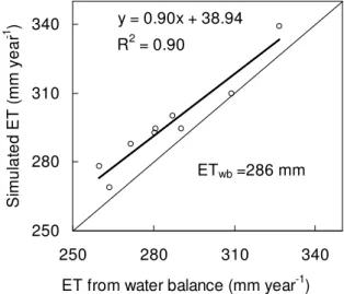
R2 = 0.90
y = 0.90x + 38.94
250 280 310 340
250 280 310 340
ET from water balance (mm year-1)
S
imu
la
te
d
E
T
(
mm y
e
a
r
-1 )
ETwb =286 mm
Fig. 5.The simulated averaged annual and the observedET which
is the difference between the observed annual precipitation and dis-charge based on water balance (wb) of the 9 sub-catchments of the Wuding River basin in 2000.
tive units between the driest and wettest conditions in the pe-riod of 1 August 1991 to 31 May 2007 (data acquisition has been done irregularly with on average two measurements per week), resampled into a 12.5×12.5 km2equally-spaced dis-crete global grid, which is indicated by solid dots in Fig. 2. In the TUW algorithm, the microwave backscatter measure-ments normalized at 40◦incidence angle (σ0(40))are used to extract soil moisture dynamics. Eventually theσ0(40) mea-surements are scaled between the lowest and highest values ever observed within the long-term observations represent-ing the driest and wettest conditions. In this way, theσ0(40) corresponds to the relative soil moisture values at topmost 2–5 cm soil surface ranging between 0 and 1 (0% and 100%) (Naeimi et al., 2009).
3.2.2 Meteorological and hydrological data from 1956 to 2004
The climatic data at 15 stations in and around the basin from 1956 to 2004 are used to drive the model. The atmospheric forcing variables are daily maximum and minimum air tem-perature, humidity, wind speed, precipitation and sunshine duration. The daily climatic data are interpolated to the whole basin with the inverse distance square method. Dis-charge data from the 9 sub-catchments from 1956 to 2004 are used for model validation.
3.2.3 Land surface characterization data
0.07 0.11 0.15 0.19
1 3 5 7 9 11
θ
1
(c
m
3 cm -3)
0.15 0.2 0.25
1 3 5 7 9 11
CV
of
θ
1
0.08 0.12 0.16
1 3 5 7 9 11
θ
2
(c
m
3 cm -3)
0.14 0.17 0.2
1 3 5 7 9 11
CV
of
θ
2
θ
θ
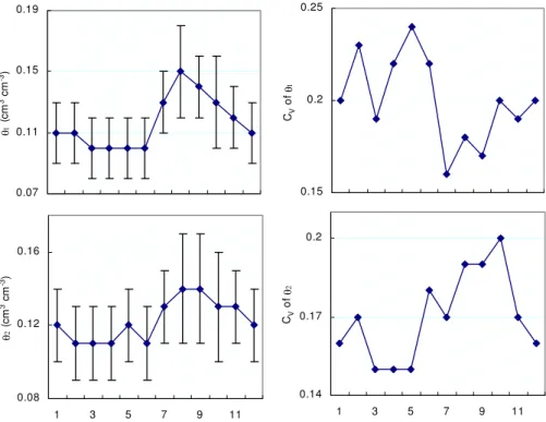
Fig. 6. Seasonal cycle (left panel) of monthly mean SM in the 0–2 cm surface layer (θ1)and root zone (θ2)averaged over the entire data
records (1957–2004) and their variability (right panel). Months are indicated with the numbers on the abscissa. Shown in the figure is also the one standard deviation.
resolution terrain raster. Leaf Area Index (LAI) mainly features the vegetation density, which is estimated by the VIP model. Soil texture data are retrieved from the map at the scale of 1:14 000 000 (Institute of Soil Science, Chi-nese Academy of Sciences, 1986). Land use data at the scale of 1:100 000 (http://www.resdc.cn/) in 1980s are used for land-use/cover classification, which is divided into six types, namely, farmland, mixed forest, dwarf shrub, grassland and desert with fractions of 29%, 3%, 4%, 43% and 21%, re-spectively. Farmland is mainly located in the stream valleys, slopes and terraces in the southern part, on which crops, such as maize, millet, soybean, rice and wheat, are planted. Natu-ral vegetation cover in the basin is geneNatu-rally sparse. Excess reclamation and over-grazing have induced vegetation degra-dation, soil erosion and desertification, which are the main causes of environmental vulnerability in this basin.
3.3 Model implementation and analysis
Water and energy balance components are calculated for each grid point separately, neglecting flux exchanges be-tween the grid points. Since the irrigated field covers only a small amount of the farm land area, the farm land is consid-ered as fully rain-fed land. As the energy fluxes’ response to atmospheric driving forces is much faster than the response of hydrological processes in the soil, the energy budget mod-ule is run on hourly basis and soil water modmod-ule on daily intervals.
Geographical and vegetation cover data are sampled re-spectively into the VIP grid resolution of 8 km. The reason of using 8 km sampling is to be in harmony with the resolu-tion of global NDVI data from NOAA.
The data time period is from 1956 to 2004. The model is validated over the period of 1991–2004, by using SM ob-servations in ten-day intervals at two in-situ stations and re-motely sensed SM data grid by grid over the basin with at least two measurements per week on average.
Both the modeled and in-situ SM data are scaled with TUW scatterometer data to have uniform datasets by using the following formulations for the validation.
RangeVIP= max(SMVIP)−min(SMVIP) Rangeobs= max(SMobs)−min(SMobs) RangeTUW= max(SMTUW)−min(SMTUW) SMVIP normalizedi =(SMVIPi −min(SMVIP))
×RangeTUW/RangeVIP+min(SMTUW) SMobs normalizedi =(SMobsi −min(SMobs))
×RangeTUW/Rangeobs
+min(SMTUW)
(13)
0 2 4 6
1 3 5 7 9 11
P
(mm)
0 0.4 0.8 1.2 1.6
1 3 5 7 9 11
CV
of
P
-20 0 20 40
1 3 5 7 9 11
T (
oC
˅
0 0.3 0.6 0.9
1 3 5 7 9 11
CV
of
T
0 50 100 150
1 3 5 7 9 11
Q
˄m
3 s -1)
0 0.2 0.4 0.6
1 3 5 7 9 11
CV
of
Q
Fig. 7.Seasonal cycle (left panel) of precipitation (P ), air temperature (T )and runoff (Q)at the control station of the basin averaged over the entire data records (1957-2004) and their variability (right panel). Months are indicated with the numbers on the abscissa. Shown in the figure is also the one standard deviation.
These VIP SM data are used to compare with the correspond-ing TUW data.
By using the validated model, the SM is simulated from 1956 to 2004. One simulation year of 1956 is repeated to avoid of the possible influence of initial status in the beginning of the modelling. The trend analysis was per-formed using the M-K and Sen’s methods after spatially av-eraging the long-term SM over the whole basin. The sea-sonal patterns of all CEH variables are compared with each other. Coefficient of variation (CV, Liu et al., 2001) is used
to make further analysis of the temporal characteristics of the SM variation.
4 Results
4.1 Validation of the model
-1 0 1 2 3 4 5
1 3 5 7 9 11
Rn
(
mm)
0 1 2 3 4 5
1 3 5 7 9 11
CV
of
R
n
0 1 2 3 4
1 3 5 7 9 11
ET
(m
m
)
0.1 0.2 0.3 0.4
1 3 5 7 9 11
CV
of
E
T
0 1 2 3
1 3 5 7 9 11
E
C
(m
m
)
0.1 0.3 0.5 0.7 0.9
1 3 5 7 9 11
C
V
of
E
C
Fig. 8a.Seasonal cycle (left panel) of net radiation (Rn), total evapotranspiration (ET), canopy transpiration (EC), averaged over the entire
data records (1957∼2004) and their variability (right panel). Months are indicated with the numbers on the abscissa. Shown in the figure is also the one standard deviation.
by some authors that the utility of the Nash-Sutcliffe effi-ciency as a performance measure may be limited by bias in its evaluation (Garrick et al., 1978; Ma et al., 1998; Weglar-czyk, 1998; Sauquet and Leblois, 2001), especially because the square summation between the observation and the sim-ulation is not necessarily smaller than the square summation (σ2obs)between the observation and the mean of the obser-vation, whenσ2obs is small. More details are shown in Mo et al. (2006a). Although R2 and Nash-Sutcliffe efficiency are not high in all the cases, from Fig. 3, the simulated SM data by VIP model and the TUW data can catch the variation trend and match with the observed SM at Suide and Yulin basically.
In the regional scale, the relative SM (%) averaged over 6 years (1992–1997) for both VIP simulation and TUW data are shown in Fig. 4. Generally, at regional scale the averaged
simulation SM data comply pretty well with the averaged TUW data except in winter period in which some obvious discrepancies are observable. In winter the simulated SM values are larger than the values of TUW data. It is worthy to mention that this cannot be treated as real large errors as the TUW data in winter should be used in caution. The rea-son is that the backscatter from frozen soil surface behaves like the backscatter from dry soil. Depending on the wetness of snow cover, backscatter signal changes sporadically under this kind of condition. It is very difficult to predict the be-havior of backscatter from a surface covered with snow and frozen soil (Albergel et al., 2009).
Validation is also done based on observed discharge data indirectly. The estimated annual ET from the VIP model
is compared with the observed annual ET, which is the
0 0.4 0.8 1.2
1 3 5 7 9 11
ES
(
mm)
0 0.1 0.2 0.3 0.4
1 3 5 7 9 11
C
V
of
E
S
0 0.06 0.12 0.18
1 3 5 7 9 11
E
I
(
mm )
0.1 0.4 0.7 1
1 3 5 7 9 11
C
V
of
E
i
0 0.5 1 1.5 2
1 3 5 7 9 11
L
AI
0 0.3 0.6 0.9
1 3 5 7 9 11
C
V
of
L
AI
Fig. 8b.Same as Fig. 8a, but for soil evaporation (ES), evaporation form the intercepted precipitation by the canopy (EI)and leaf area index
(LAI).
discharge. Figure 5 shows the comparison in one of the vali-dated years from the 9 sub-catchments withR2being 0.90.
4.2 The seasonal variation and multi-year variability of SM at daily and monthly scales
Before studying the general trend of the SM over the recorded years, it is meaningful to detect the variation of SM at temporal scales including the daily, monthly, annual and decadal scales.
We first look at the seasonal cycle of SM and its multi-year variability (Fig. 6). It is seen that SM follows the summer monsoon pattern in that the maximum SM both for surface and root zone happens in summer, so do SM for all other CEH variables as shown in Figs. 7 and 8a, b. During spring, over the basin, SM is relatively stable. There is a sharp de-crease of soil water from February to March (in surface) or from January to February (root zone), because the lowest
temperature in the basin is not in December, but in January (Fig. 7). This makes the soil surface or the whole of soil profile frozen, with a little lag over the basin, causing the minimum SM occurred in the earlier spring. The small peak of root-zone SM in May is corresponding to warmer weather (higher temperature in Fig. 7), which makes SM higher. This also causes the spring flood in runoff (Qin Fig. 7), but it hap-pens in March, as the surface water (river) gets warm earlier than the soil water.
0.1 0.2 0.3 0.4 0.5
1
32 63 94
125 156 187 218 249 280 311 342
DOY(Jan1-Dec.31)
CV
of
θ
1
0.06 0.1 0.14 0.18
1 32 63 94
12
5
15
6
18
7
21
8
24
9
28
0
31
1
34
2
DOY (Jan1-Dec.31)
θ
1
(c
m
3 cm -3)
0.1 0.15 0.2 0.25 0.3
1
32 63 94
125 156 187 218 249 280 311 342
DOY(Jan1-Dec.31)
CV
of
θ
2
0.1 0.12 0.14 0.16
1
32 63 94
125 156 187 218 249 280 311 342
DOY(Jan1-Dec.31)
θ
2
(c
m
3 cm -3)
θ θ
Fig. 9.Mean daily SM (left panel) and SM variability (right panel) at daily time scale in the 0–2 cm surface layer (θ1)and root zone (θ2).
Day 1=1 January.
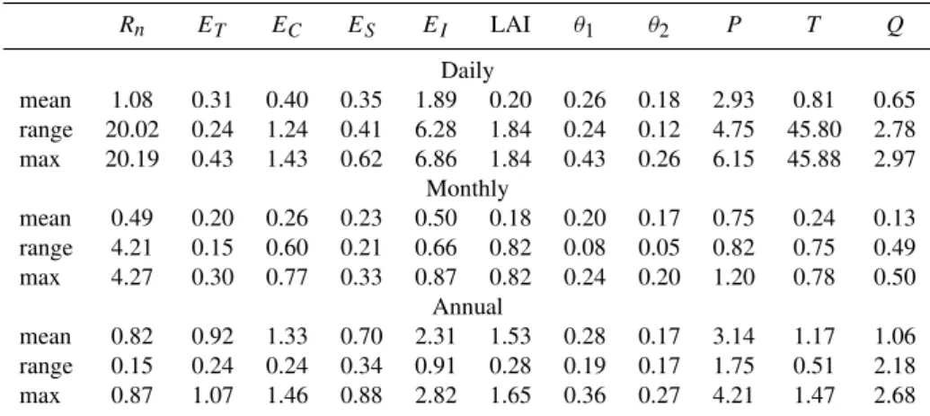
Table 1.The mean, range (=max-min) and the maximum ofCvfor the 11 CEH variables at the daily, monthly and annual scale.
Rn ET EC ES EI LAI θ1 θ2 P T Q
Daily
mean 1.08 0.31 0.40 0.35 1.89 0.20 0.26 0.18 2.93 0.81 0.65 range 20.02 0.24 1.24 0.41 6.28 1.84 0.24 0.12 4.75 45.80 2.78 max 20.19 0.43 1.43 0.62 6.86 1.84 0.43 0.26 6.15 45.88 2.97
Monthly
mean 0.49 0.20 0.26 0.23 0.50 0.18 0.20 0.17 0.75 0.24 0.13 range 4.21 0.15 0.60 0.21 0.66 0.82 0.08 0.05 0.82 0.75 0.49 max 4.27 0.30 0.77 0.33 0.87 0.82 0.24 0.20 1.20 0.78 0.50
Annual
mean 0.82 0.92 1.33 0.70 2.31 1.53 0.28 0.17 3.14 1.17 1.06 range 0.15 0.24 0.24 0.34 0.91 0.28 0.19 0.17 1.75 0.51 2.18 max 0.87 1.07 1.46 0.88 2.82 1.65 0.36 0.27 4.21 1.47 2.68
Note: ForRn, not include the four large values (41.47, 381.43, 131.1, 456.92) when doing the calculation.
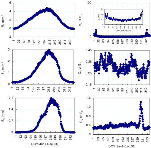
to the maximum LAI, water demand of plants is high. Due to intensive precipitation during this period, high SM condi-tion is lasting. Since the amount of precipitacondi-tion is lower in September than in August, SM is also tending to decrease.
The maximum ofET happens in August, which is matched
with the maximum of net radiation (Rn)and precipitation
(P )(Fig. 8a, b). The components ofET from canopy (EC)
and intercepted water by vegetation (EI)reach the maximum
values in August and September, which are corresponding to
the high LAI in September due to high water consumption by the vegetation. AlthoughES also reaches the highest in
summer due to high temperature and precipitation, its max-imum does not happen in September when the leaf covers fully. The maximum ofES reaches maximum in July when
there are much water in soil surface for evaporation. The ra-tio ofECtoET is much higher than the ratio ofEStoET in
the growing season, which makes the pattern of totalET
0 2 4 6 8
1
32 63 94
125 156 187 218 249 280 311 342
DOY(Jan1-Dec.31)
CV
of
P
0 2 4 6 8
1 32 63 94
12
5
15
6
18
7
21
8
24
9
28
0
31
1
34
2
DOY (Jan1-Dec.31)
P
˄mm)
0 10 20 30 40 50
1
32 63 94
125 156 187 218 249 280 311 342
DOY(Jan1-Dec.31)
CV
of
T
-10 0 10 20 30
1
32 63 94
125 156 187 218 249 280 311 342
DOY(Jan1-Dec.31)
T (
oC
˅
0 1 2 3 4
1
32 63 94
125 156 187 218 249 280 311 342
DOY(Jan1-Dec.31)
CV
of
Q
0 40 80 120 160
1
32 63 94
125 156 187 218 249 280 311 342
DOY(Jan1-Dec.31)
Q (
m
3 s -1)
Fig. 10. Mean daily values (left panel) and their variability (right panel) at daily time scale for precipitation (P ), air temperature (T )and runoff (Q)at the control station of the basin. Day 1=1 January.
is opposite in winter, where the values for bothET and the
components are small.
The patterns ofCV can be categorized into two groups.
The first is theCV patterns essentially matching with the
pat-terns of the variables, such as root Zone SM,Q, LAI, and EC. The second is theCV patterns being right opposite to
the patterns of the variables, such as surface SM,P,T,Rn,
ET,ES andEI. For each pattern, the time for the peak (or
trough) appearance of the variable is not necessarily matched with the time for that of theCv.
Generally, the multi-year variability of SM over the 48 years (1956–2004) is the least compared with other CEH variables (Table 1). Over the years, runoff at the cross-section of the basin has been used as an important index for trend analysis because of the relative easy data access (e.g., Zhang et al., 1998; Qian et al., 1999; Xu, 2004; Li et al.,
2007). However, strong variation of runoff itself may make it hard to get a trend. Compared with runoff, SM, with lower multi-year variability, may be a better and important hydro-logical component to explore the changes of hydrohydro-logical el-ements in the Wuding River basin. This encourages us using SM to describe the CEH trend in the basin.
0 100
1
32 63 94 125 156 187 218 249 280 311 342
DOY (Jan1-Dec.31)
CV
of
R
n
-2 0 2 4 6
1
32 63 94 125 156 187 218 249 280 311 342
DOY (Jan1-Dec.31)
Rn
(m
m
˅
0 1 2 3
1
32 63 94
12
5
15
6
18
7
21
8
24
9
28
0
31
1
34
2
DOY (Jan1-Dec.31)
ET
(m
m
˅
0.15 0.25 0.35 0.45
1 32 63 94
12
5
15
6
18
7
21
8
24
9
28
0
31
1
34
2
DOY (Jan1-Dec.31)
CV
of
E
T
0 0.7 1.4 2.1
1
32 63 94
125 156 187 218 249 280 311 342
DOY (Jan1-Dec.31)
EC
(
mm)
0 0.4 0.8 1.2 1.6
1
33 65 97 129 161 193 225 257 289 321 353
DOY (Jan1-Dec.31)
CV
of
E
C
0 0.3 0.6 0.9
30 61 92 123 154 185 216 247 278 309
DOY(Jan1-Dec.31)
C
V
of
R
n
Fig. 11a.Mean daily values (left panel) and their variability (right panel) at daily time scale for net radiation (Rn), total evapotranspiration
(ET)and canopy transpiration (EC). Day 1=1 January.
toET, being influenced more comprehensively by both the
atmospheric forcing and vegetation dynamics (Fig. 8). No matter how high or low the variability of SM in sum-mer is, the seasonal variation ofCV for surface and root zone
SM is obvious, a feature in rainfed situation as in our case. For irrigation case instead, theCV’s variation is much
sta-ble (Mahmood and Hubbard, 2004). Under variasta-ble hydro-climatic condition (precipitation and temperature), plant de-mand of moisture and insufficient water supply result in the alternative peak and minimum pattern of SM variability.
By comparing the seasonal cycle and its variability with the monthly (Figs. 6–8 ) and daily SM (Figs. 9–11), it is seen that the seasonal cycles are similar to both the SM and other CEH variables. As expected, changes in SM from one to the next month are not as drastic as those at the daily scale. Over-all, the monthly variability is relatively “smooth” compared to that at daily scale, with the means ofCV at the monthly
scale being less than the means ofCV at the daily scale for
all the variables (Table 1, and Fig. 12). More fluctuating local hydro-climatic conditions at daily scale, namely, wet or dry, are averaged monthly, reducing SM variability at monthly scales. As some variability has been averaged, some
pat-terns are clearer at monthly than at daily scale. For example the double peak of runoff and SM is shown clearly at the monthly scale, which is hid at the daily scale.
From Fig. 12, it is shown that the values ofCV of SM at
daily, monthly and yearly scale are all smaller than those of other CEH variables. Lower variability in SM can be ex-plained at least in the following two courses. Firstly, the Wuding River basin is located in a semi-arid climate zone where annual precipitation is about 400 mm yr−1and most of it falls in summer. The low precipitation leads to low sur-face SM, which is close to the wilting point. Secondly, scien-tists found that owing to its larger inertia and longer memory to atmospheric driving force than other hydrological com-ponents, SM, along with snow cover, is the most important component of meteorological memory for the climate system over the land (Delworth and Manabe, 1988, 1993; Robock et al., 2000). All of these support our first impression to the low variability of SM in the Wuding River basin.
It is worthy to point out that the value of the variable, its standard deviation and itsCV should be used conjunctively
0 0.4 0.8 1.2
1
32 63 94 125 156 187 218 249 280 311 342
DOY (Jan1-Dec.31)
ES
(
mm)
0.1 0.3 0.5 0.7
1
32 63 94 125 156 187 218 249 280 311 342
DOY (Jan1-Dec.31)
CV
of
E
S
0 2 4 6 8
1 32 63 94
12
5
15
6
18
7
21
8
24
9
28
0
31
1
34
2
DOY (Jan1-Dec.31)
CV
of
E
I
0 0.05 0.1 0.15 0.2
1 32 63 94
12
5
15
6
18
7
21
8
24
9
28
0
31
1
34
2
DOY(Jan1-Dec.31) EI
˄mm
)
0 0.5 1 1.5 2
1
32 63 94
12
5
15
6
18
7
21
8
24
9
28
0
31
1
34
2
DOY (Jan1-Dec.31)
CV
of
L
AI
0 0.6 1.2 1.8
1
32 63 94 125 156 187 218 249 280 311 342
DOY (Jan1-Dec.31)
LAI
Fig. 11b.Same as Fig. 11a but for soil evaporation (ES), evaporation from the intercepted precipitation by the canopy (EI)and leaf area
index (LAI).
2001; Mahmood and Hubbard, 2004). For example, the stan-dard deviation ofRn in summer is larger than that in winter
season. However, theCV in summer is the lowest. Usually,
the relationship between the standard deviation and the value is positive and the relationship betweenCV and the variable
itself (and the standard deviation) is negative (Fig. 13). There is a minor shortcoming in usingCV for variability analysis.
For example, when the value is turning from negative to pos-itive or vice versa, such as in theRnandT cases (Figs. 7 and
8, Figs. 10, 11), the value ofCV is much higher than what is
expected. When the value is at the turning point from high to low and when the mean values are very low, such as in the LAI andECcases, theCV values are also very high.
How-ever, this is not really meaning that the multi-year variability at this time is much larger than that in other periods.
4.3 The interannual variation of SM and its variability within each year
The interannual variation of SM and its within-year variabil-ity are shown in Fig. 14. There is a decreasing tendency for SM both in the surface and the root zone. Year 1999 is the
driest among the simulation years. The within-year variabil-ity keeps the same over the years, also seen in Fig. 15. This pattern follows that of precipitation. So does for runoff. We can see that although the values of SM,P and runoff (Q) are in decreasing tendency, their within-year variability keeps relatively stable. Comparing withP,Qand all other CEH variables (Figs. 16 and 17 and Table 1), the within-year vari-ability of SM is the least. This again encourages us using SM to explore the change signal of CEH processes in the basin.
It is clear that over the years, the basin is getting warmer, but the within-year variation of temperature is get-ting smaller, showing that the seasonal cycle of temperature is weakened over the years. Over the years,Rn,ET and its
components remain stable, which shows the compensation effect of precipitation and temperature.
Table 2.The decade mean of SM (the first line) and the ratio of the difference between the decade mean and the multi-year average to the multi-year average (the second line) for precipitation (P ), net radiation (Rn), evapotranspiration (ET)and its components, GPP, NPP, runoff
(Q), root zone SM (θ2)and air temperature (T )of the Wuding River basin.
P Rn ET EC ES EI GPP NPP Q θ2 T
1950s 502.3 776.4 442.3 237.2 193.3 11.9 42.2 243.0 103.7 0.12 9.73 0.16 0.00 0.09 0.10 0.07 0.05 0.04 0.18 0.72 0.05 −0.03 1960s 482.8 785.9 421.5 216.2 194.2 11.1 37.2 188.1 93.7 0.1 9.73
0.11 0.01 0.03 0.00 0.08 −0.02 −0.09 −0.08 0.56 0.12 −0.03 1970s 422.9 773.7 402.8 213.1 178.1 11.6 38.9 199.5 55.8 0.1 9.83
−0.02 0.00 −0.01 −0.01 −0.01 0.03 −0.05 −0.03 −0.07 0.03 −0.02
1980s 418.5 762.7 403.9 216.0 176.7 11.2 42.3 213.4 49.5 0.1 9.80
−0.03 −0.02 −0.01 0.00 −0.02 −0.01 0.04 0.04 −0.18 −0.03 −0.02
1990s 392.9 777.4 391.8 212.7 168.1 11.0 43.1 209.0 36.2 0.1 10.6
−0.09 0.00 −0.04 −0.02 −0.07 −0.03 0.06 0.02 −0.40 −0.11 0.05
2000s 424.9 777.5 408.1 217.4 179.1 11.6 42.6 203.4 45.1 0.1 10.74
−0.02 0.00 0.00 0.01 −0.01 0.03 0.05 −0.01 −0.25 −0.02 0.07
0 1 2 3 4
Rn ET EC ES EI LAI q1 q2 P T Q
Me
a
n
o
f C
v
Daily Monthly Annual
θ
θ
Fig. 12.The mean of theCV at the daily, monthly and annual scale
(q1 andq2 representsθ1and θ2, respectively). ForRn, the four
large values (41.47, 381.43,131.1, 456.92) are not included.
rate of 0.00072 kg kg−1based on the observed data from 13 stations from 1981 to 1998.
One interesting phenomenon is that the decreasing ten-dency of precipitation has been shown in 1970s already, so does runoff with an immediate correspondence. However, the decreasing tendency of SM has a delay, which appears only in late of 1980s. This shows that there is a lag in SM’s response to precipitation.
4.4 The total variation trend of SM over the 48 years
The M-K method is used to explore how significant of the trend is. Although there is a suggestion to use the SM in summer (June, July, August) to test the trends of SM as sum-mer drying will accompany global warming (Robock et al., 2005), the annual mean SM is used in the trend analysis in a more comprehensive way.
Some studies made the variables standardized/normalized at first before they did the trend analysis (Zhao and Yan, 2006). Scaling the axes, or standardizing the variables is a common technique (e.g., Liu et al., 2001; Ouarda et al., 2001; Mo and Beven, 2004; Riad et al., 2004). Application of such
0 2 4 6 8 10
0 10 20 30 40 50
The mean value
The m
ean
s
tde
v
0 2 4 6 8 10
0 0.2 0.4 0.6 0.8
The mean CV
Th
e m
e
an s
tde
v
0 10 20 30 40 50
0 0.2 0.4 0.6 0.8
The mean CV
The m
ean
s
tde
v
Table 3. The statistics of M-K trend and Sen’s slope estimate for the 11 CEH variables by using original M-K, M-K with prewhitening by von Stroch, Zhang and Yue method respectively. (Zandµare explained in Sect. 2.2.ρ1is the lag-1 auto-correlation coefficient).
Original M-K M-K by von Storch M-K by Zhang M-K by Yue
ρ1 Z Sig. µ ρ1 Z Sig. µ ρ1 Z Sig. µ ρ1 Z Sig. µ
(1) (2) (3) (4) (5) (6) (7) (8) (9) (10) (11) (12) (13) (14) (15) (16)
P −0.15 −1.72 d −0.020 0.02 −2.35 c −0.027 −0.25 −2.42 c −0.028 −0.01 −2.02 c −0.024
Rn −0.06 −1.03 −0.011 −0.01 −1.01 −0.011 −0.06 −1.01 −0.011 −0.01 −0.97 −0.010
ET 0.30 −1.54 −0.018 0.05 −0.62 −0.006 0.27 −0.70 −0.007 0.08 −1.03 −0.012
EC 0.12 −0.42 −0.006 0.06 0.00 0.001 0.13 0.00 0.001 0.07 0.00 0.000
ES 0.41 −2.07 c −0.026 0.05 −1.34 −0.013 0.33 −1.39 −0.016 0.13 −2.22 c −0.024
EI −0.41 −0.35 −0.004 −0.02 0.11 0.001 −0.41 0.11 0.001 −0.02 0.37 0.003
GPP 0.07 3.10 b 0.034 0.00 3.08 b 0.034 −0.19 4.04 a 0.044 0.03 3.26 b 0.037
NPP −0.23 0.65 0.009 0.00 1.83 d 0.017 −0.25 1.91 d 0.018 −0.02 1.65 d 0.015
Runoff 0.08 −3.33 a −0.019 0.00 −3.01 b −0.018 −0.14 −3.76 a −0.026 0.02 −3.19 b −0.020
θ2 0.20 −2.83 b −0.031 0.03 −2.94 b −0.031 0.04 −2.94 b −0.031 0.10 −3.34 a −0.037
T 0.42 3.39 a 0.035 −0.05 1.80 d 0.022 0.23 2.55 c 0.029 0.12 3.08 b 0.037
aif trend atα=0.001 level of significance;bif trend atα=0.01 level of significance;cif trend atα=0.05 level of significance;dif trend at
α=0.1 level of significance
Table 4. The final estimate of the trend and its significance for each of all the 11 CEH variables (the significance of linear trend and the lag-1 autocorrelation coefficientρ1, as shown in columns 4 and 6, are assessed by the method as described in Yue et al. (2002). The ratio of column 2 and column 3 is the standard deviation of the years from 1956 to 2004, i.e., 14. The meaning of symbol of the significance is the same as in Table 3).
Linear trend Lag-1 cor The final estimate of trend Var. Original time scale Standardized time scale Sig. ρ1 Sig. Z Sig µ
(1) (2) (3) (4) (5) (6) (7) (8) (9)
P −0.2886 −0.021 d −0.15 −1.715 d −0.020
Rn −0.0972 −0.007 −0.06 −1.031 −0.011
ET −0.2378 −0.017 0.295 c −1.027 −0.012
EC −0.0897 −0.006 0.124 −0.418 −0.006
ES −0.3462 −0.025 c 0.411 b −2.219 c −0.024
EI 0.0072 0.0005 −0.41 b 0.367 0.003
GPP 0.4381 0.0313 b 0.074 3.102 b 0.034
NPP 0.0837 0.006 −0.23 0.649 0.009
Runoff −0.4345 −0.031 b 0.076 −3.333 a −0.019
θ2 −0.3877 −0.028 c 0.204 −2.826 b −0.031
T 0.546 0.039 a 0.423 b 3.081 b 0.037
aif trend/correlation atα=0.001 level of significance, for correlation coefficient,lower bound=-0.49, upper bound=0.45 bif trend/correlation atα=0.01 level of significance, for correlation coefficient,lower bound=-0.39, upper bound=0.35
cif trend/correlation atα=0.05 level of significance, for correlation coefficient,lower bound=-0.30, upper bound=0.26 dif trend/correlation atα=0.1 level of significance, for correlation coefficient,lower bound=-0.26, upper bound=0.22
transformations prior to the analysis attempts to remove the influence of scaling effects from the analysis, with the aim to obtain a simpler expression (Ouarda et al., 2001). Further-more, when plotting the results for a large number of catch-ments, variables with the largest means tend to dominate the display. As discussed by Friendly and Kwan (2003), scaling axes can obviously lead to an incoherent display in which no systematic trends or relations can be distinguished.
There-fore although as shown in Liu et al. (2008), scaling may bring the uncertainty of the results, we still use the normalized SM for trend analysis, in order to make a better comparison with other CEH variables.
y = -0.0005x + 0.1303
R2 = 0.2025
0.07 0.11 0.15 0.19
1957 1967 1977 1987 1997
θ
1
(c
m
3 cm -3)
y = 0.0008x + 0.2565
R2 = 0.0563
0.15 0.25 0.35 0.45
1957 1967 1977 1987 1997
CV
of
θ
1
y = -0.0004x + 0.1335
R2 = 0.207
0.08 0.12 0.16
1957 1967 1977 1987 1997
θ
2
(c
m
3 cm -3)
y = -0.0003x + 0.1795
R2 = 0.0118
0.05 0.15 0.25 0.35
1957 1967 1977 1987 1997
CV
of
θ
2
θ
θ
Fig. 14. The annual mean of SM in the 0–2 cm surface layer (θ1)and root zone (θ2)(left panel) and their variability (right panel) over the
years.
and without prewhitening, a linear trend and its significance are also calculated based on standardized dataset. The results are shown in Table 3.
Generally, in most of the cases, no matter which prewhitening techniques are used, they all lead to potentially inaccurate assessments of the significance of a trend. In most cases forP, Rn,ET,EC,ES, andT, they follow the same
pattern as those deducted from numeric experiments (Yue et al., 2002; Zhang et al., 2004). That is, removal of positive lag-1 auto-correlation from the data by prewhitening will re-move a portion of trend and hence reduce the possibility of rejecting the null hypothesis while it might be false. Contrar-ily, removal of negative lag-1 auto-correlation by prewhiten-ing will inflate trend and lead to an increase in the possibility of rejecting the null hypothesis while it might be true (Yue et al., 2003). For those not following the above pattern, it may be due to either the very small trend as in theEI and NPP
cases, or the large trend with smallρ1as in the cases of GPP
and Runoff.
However, for all techniques, as shown in Fig. 18 and Ta-ble 3, the differences of the estimates of the trends are not very much. The final estimate of the trend is depended on the significance of the auto-correlation coefficient. The significance is assessed using the same method as in Yue et
al. (2003). When the data are not autocorrelated significantly, the trend from original M-K and Sen method is used. When the data are autocorrelated significantly, we choose the trend from the three techniques, which most approaches the origi-nal trend and with lowestρ1. The final estimate of the trend
and its significance for each of all the 11 CEH variables are shown in Table 4.
Although the least square estimator of linear trend is vul-nerable to gross errors and the associated confidence interval is sensitive to non-normality of the parent distribution (Sen, 1968, from Wang and Swail, 2001), it is still used to make a comparison with the final estimate of trend. It is found that after normalizing both the variable and time (year), the cor-relation between the variable and the time is right equal to the linear trend of the normalized variable at the normalized time scale (column 3 in Table 4). It is thus possible to use the same method of assessment of the significance of corre-lation to assess the significance of the linear trend, as shown in column 4 in Table 4.
From Table 4, it is shown that the Wuding River basin is in drying tendency atα=0.01 level of significance. Runoff, pre-cipitation and soil evaporation (ES)are also in a decreasing
1 3 5 7 9 11 Month
1957 1962 1967 1972 1977 1982 1987 1992 1997 2002
Fig. 15.Year/month plot of SM variations in the root zone, averaged over the Wuding River basin.
soil evaporation (α=0.05). Temperature is in increasing ten-dency at the same level of significance as SM. The tenten-dency of net radiation (Rn), Evapotranspiration (ET), transpiration
(EC), canopy intercept (EI)is not obvious in that the M-K
test indicates a decreasing trend forRn,ET andEC and
in-creasing trend for EI, but all at the less significance level
thanα=0.1. As the trend forEIis very small, prewhitening
techniques are possible to change the direction of the trend. Thus for a small trend, discussion on its direction has no re-alistic meaning.
It is interesting to see from Table 4 that although soil is in drying tendency, vegetation productivity (NPP (net primary productivity), especially GPP (gross primary productivity)) is in increasing tendency. It is seen that the temperature is in increasing tendency. In North China, it is found that if no CO2 fertilization effect is considered, crop yield is reduced
with an increase in temperature (Liu et al., 2009). However, if considering CO2fertilization, crop yield may increase. As
our model not only deals with hydrological process, but also with vegetation dynamics, the response of productivity may be affected by the precipitation, CO2fertilization and
tem-perature. It is thus understandable why a drier soil may pro-duce higher vegetation productivity.
It is worthy to mention that, although the absolute value of SM trend is small, the normalized trend of SM is large (Fig. 18). This indicates that northern drying is an important signal in the basin.
5 Discussions
5.1 Northern drying?
The drying tendency in the north of China, Northern Drying, has been paid strong attention to. Tao et al. (2003) produced a long-term SM dataset over China, represented by soil deficit index, from 1946 to 1995 by using a conceptual model. They found there was a trend toward soil drying in the North China Plain and the North-eastern China area during this period. By using the observed SM data from 35 stations over North China from 1981 to 2002, Zhao and Yan (2006) found that the whole trends of annual mean SM storage averaged by different soil layers from soil surface to top 50 cm was de-creasing generally. By using SM dataset of the top 50-cm soil layers at 178 SM stations in China from 1981 to 1998, Nie et al. (2008) found that there were increasing trends of SM for the top 10 cm, but decreasing trends for the top 50 cm of soil layers in most regions. Our study further identifies this Northern Drying phenomenon.
The same drying trend is also found in West Africa, as driven by decreasing Sahel precipitation. For most of other areas in the world and in some parts of China, the trends are different. For example in Ukraine, Russia, Mongolia (Robock, 2000; Robock and Li, 2006) and most parts of the US (Robock, 2000; Andreadis and Lettenmaier, 2006; Sheffield and Wood, 2008), soil is found in wetter tendency. In the far North China Qaidam Basin of Qinghai Province in northwestern China, Yin et al. (2008) reconstructed the SM conditions from tree ring from year 566 to 2001 and re-vealed a general trend toward a wetter condition during the most recent 300 years. Tao et al. (2003) reported that there was a significant increase in SM levels in Southwest China, and a generally insignificant increase or decrease trend in SM levels in Southeast China. Europe, southeast and southern Asia appears to having not experienced significant changes in SM (Sheffield and Wood, 2008).
5.2 Man-made Northern drying or nature-made
The definitions of man-made and nature-made change in dif-ferent disciplines are not the same. For example, from clima-tology’s view, man-made change includes a) local changes such as land use, b) large-scale changes that caused by an-thropogenic forcing such as global warming. And the nature made changes include a) natural internal variation of the cli-mate system and b) natural forcing external to earth clicli-mate system such as changes in solar output. In this paper, we only pay attention to the regional-local land use change as man-made change and natural internal variation of the cli-mate system as the nature-made change.
y = -0.0055x + 1.3214
R2 = 0.0855
0 0.5 1 1.5 2 2.5
1957 1967 1977 1987 1997
P
˄mm)
y = 0.0031x + 3.0679
R2 = 0.0138
2 3 4 5
1957 1967 1977 1987 1997
CV
of
P
y = 0.0255x + 9.4203
R2 = 0.2981
8.5 9.5 10.5 11.5
1957 1967 1977 1987 1997
Τ
˄
οC
)
y = -0.0039x + 1.2598
R2 = 0.2757
0.9 1.1 1.3 1.5
1957 1967 1977 1987 1997
CV
of
T
y = -0.5685x + 50.81
R2 = 0.5628
0 10 20 30 40 50 60 70
1957 1967 1977 1987 1997
Q (
m
3 s -1)
y = 0.001x + 1.0378
R2 = 0.0006
0.15 1.15 2.15 3.15
1957 1967 1977 1987 1997
CV
of
Q
Fig. 16.The annual mean of precipitation (P ), air temperature (T )and runoff (Q)at the control station of the basin (left panel) and their variability (right panel) over the years.
to conserve soil and water, it has taken many soil water con-servation countermeasures, including planting trees, build-ing terraces and constructbuild-ing checkbuild-ing dams. These counter-measures not only mitigate the sediment yield from the basin but also change the hydrological processes in the basin via land use and cover change (LUCC). Therefore any chang-ing tendency from the observed data may be contributed by human activities or climate change. It is a big challenge to distinct their contributions. There are some methods such as “baseline” method (Lorup et al., 1998; Yang et al., 2005; Li et al., 2007), “regression” (e.g., Xu, 2004) and “optimal fingerprint” method (Hasswlmann, 1997; Allen and Scott, 2003; Zhang et al., 2007) to deal with this problem. In our research the long-term SM data are simulated by actual
at-mospheric forcing and land cover, the trend shown by the data should reflect more the influence of nature factors.
The decrease in precipitation seems the primary reason for the trend of SM. Logically, with the increase in temperature in Wuding River, ET may increase consequently, and will
further reduce the soil water storage. However in our case the totalET and canopy transpiration shows a declining trend at
an insignificant level. Soil evaporation shows a downward trend at the significant level ofα=0.05. Actually,ET is not
linearly related with temperature as described by VIP, which plays a complicate role in temperature-ET -SM relationship.
In this semi-arid basin, annual ET is mainly regulated by
y = -0.0005x + 2.1352
R2 = 0.0107
1.9 2.1 2.3 2.5
1957 1967 1977 1987 1997
Rn
(mm)
y = -0.0005x + 0.8331
R2 = 0.0844
0.7 0.78 0.86 0.94
1957 1967 1977 1987 1997
CV
of R
n
y = -0.0019x + 1.1626 R2 = 0.0548
0.7 0.9 1.1 1.3 1.5
1957 1967 1977 1987 1997
ET
(mm)
y = 0.0007x + 0.9006
R2 = 0.0427
0.8 0.9 1 1.1
1957 1967 1977 1987 1997
CV
of E
T
y = -0.0005x + 0.604 R2 = 0.0072
0.3 0.5 0.7 0.9
1957 1967 1977 1987 1997
EC
(mm)
y = -0.0014x + 1.3663 R2 = 0.1135
1.2 1.3 1.4 1.5
1957 1967 1977 1987 1997
CV
of E
C
Fig. 17a.The annual mean of net radiation (Rn), total evapotranspiration (ET), canopy transpiration (EC)(left panel) and their variability
(right panel) over the years.
5.3 The representative of SM simulation via VIP
Although the simulated SM from VIP mainly reflects the changes of climate, it is still a good indicator of the wet-ness status of the basin in the real world. There are at least three reasons. Firstly, from our previous study and docu-mented studies, man-made change is a main, at least half of the contribution to the change of the runoff which is showing the decreasing tendency (Mo et al., 2006; Li et al., 2007). However, for soil moisture, as it has the least coefficient of variation relative to other CEH variables, it has been used as a more effective hydrological indicator of climate change (Robock et al., 2000). Secondly, as VIP model is a dis-tributed model, it can be used to detect the soil moisture un-der different land use scenarios, which has been a worldwide
research topic. From the documented reports, it is found that there are discernible SM differences between land use or crop types planted (Cai and Wang, 2006; Yang and Rong, 2007; Yang et al, 2008). This is one of the important reasons to use VIP to simulate SM for the Wuding River. Last but not the least, from the observed records, it is shown that the crop types haven’t changed much during the last twenty years in the Wuding River basin. The land use change over that pe-riod is less than 5%. This is the reason that although we do not consider very much the temporal variation of vegetation type for SM simulation, the SM simulation still matches the observed in an acceptable way.
y = -0.0014x + 0.5291 R2 = 0.1178
0.3 0.4 0.5 0.6 0.7
1957 1967 1977 1987 1997
ES
(mm )
y = 0.0023x + 0.6444 R2 = 0.1523
0.5 0.6 0.7 0.8 0.9
1957 1967 1977 1987 1997
CV
of E
S
y = 2E-05x + 0.0307 R2 = 0.0019
0.01 0.03 0.05
1957 1967 1977 1987 1997
EI
(mm)
y = 0.0025x + 2.2467 R2 = 0.0343 1.7
1.9 2.1 2.3 2.5 2.7 2.9
1957 1967 1977 1987 1997
CV
of E
I
y = 0.0008x + 0.3165 R2 = 0.0627
0.2 0.3 0.4 0.5
1957 1967 1977 1987 1997
LAI
y = -0.0002x + 1.5374 R2 = 0.0021
1.35 1.45 1.55 1.65
1957 1967 1977 1987 1997
CV
of LAI
Fig. 17b.The same as Fig. 17a but for soil evaporation (ES), evaporation form the intercepted precipitation by the canopy (EI)and leaf area
index (LAI).
the VIP model, which reflect the temporal changes attributed more to climate and yet also reflect the spatial variation over the basin, can be assumed to represent the realistic condi-tions. The agreements between the simulated and observed SM at the stations and the regional remotely sensed SM sup-port this assumption.
6 Conclusions
The Northern Drying phenomenon is found in the Wuding River basin, China, one of areas suffering most serious wa-ter and soil loss. As the basin just has relatively short-wa-term observed soil moisture (SM) data at two stations, an eco-hydrological processes-based model (VIP model) is used to simulate the long-term daily SM data from 1956 to 2004 to explore this trend.
The model is at first validated by both the in-situ SM data at two stations and the remotely sensed SM data produced by the Vienna University of Technology (TUW). The aver-aged TUW SM data over 189 points matched with the simu-lated SM by VIP well except significant differences in winter. Although there are differences between the simulation and measured/remotely sensed SM data, their variation trends are matched each other. From the first aspect, this encourages us to use the model to simulate the long term SM data from 1956 to 2004 for the trend analysis.