Regional scale characteristics of the seasonal cycle of chlorophyll in the Southern Ocean

(1)

BGD

8, 4763–4804, 2011

Seasonal characteristics of the

Southern Ocean

S. J. Thomalla et al.

Title Page

Abstract Introduction

Conclusions References

Tables Figures

◭ ◮

Back Close

Full Screen / Esc

Printer-friendly Version Interactive Discussion

Discussion

P

a

per

|

Dis

cussion

P

a

per

|

Discussion

P

a

per

|

Discussio

n

P

a

per

|

Biogeosciences Discuss., 8, 4763–4804, 2011 www.biogeosciences-discuss.net/8/4763/2011/ doi:10.5194/bgd-8-4763-2011

Biogeosciences Discussions

This discussion paper is/has been under review for the journal Biogeosciences (BG). Please refer to the corresponding final paper in BG if available.

Regional scale characteristics of the

seasonal cycle of chlorophyll in the

Southern Ocean

S. J. Thomalla1,2, N. Fauchereau1, S. Swart1,2, and P. M. S. Monteiro1

1

Ocean Systems and Climate Group, CSIR, P.O. Box 320 Stellenbosch, 7599, South Africa

2

Department of Oceanography, UCT, Private Bag, Rondebosch, 7700, South Africa Received: 2 February 2011 – Accepted: 28 April 2011 – Published: 13 May 2011 Correspondence to: S. J. Thomalla (sandy.thomalla@gmail.com)

(2)

BGD

8, 4763–4804, 2011

Southern Ocean

Title Page

Tables Figures

◭ ◮

Back Close

Full Screen / Esc

Discussion

P

a

per

|

Dis

cussion

P

a

per

|

Discussion

P

a

per

|

Discussio

n

P

a

per

Abstract

The seasonal cycle is the mode that couples climate forcing to ecosystem produc-tion. A better understanding of the regional characteristics of the seasonal cycle ad-dresses an important gap in our understanding of the sensitivity of the biological pump to climate change. The regional characteristics of the seasonal cycle of phytoplankton

5

biomass in the Southern Ocean were examined in terms of the timing of the bloom ini-tiation, its amplitude, regional scale variability and the importance of the climatological seasonal cycle in explaining the overall variance. The study highlighted important dif-ferences between the spatial distribution of satellite observed phytoplankton biomass and the more dynamically linked characteristics of the seasonal cycle. The seasonal

10

cycle was consequently defined into four broad zonal regions; the subtropical zone (STZ), the transition zone (TZ), the Antarctic circumpolar zone (ACZ) and the marginal ice zone (MIZ). Defining the Southern Ocean according to the characteristics of its seasonal cycle provides a more dynamic understanding of ocean productivity based on underlying physical drivers rather than climatological biomass. The response of the

15

biology to the underlying physics of the different seasonal zones resulted in an addi-tional classification of four regions based on the extent of interannual seasonal phase locking and the amplitude of the integrated seasonal biomass. This characterisation contributes to an improved understanding of regional sensitivity to climate forcing po-tentially allowing more robust predictions of long term climate trends.

20

1 Introduction

Biological production and carbon export to the deep ocean, “the biological pump” is considered a major contributor to the Southern Ocean CO₂ sink removing an esti-mated 3 PgC (1 PgC=1015g of carbon) from surface waters south of 30◦_{S each year} (33 % of the global organic carbon flux) (Schlitzer et al., 2002). The Southern Oceans

25

(3)

BGD

8, 4763–4804, 2011

Southern Ocean

Title Page

Tables Figures

◭ ◮

Back Close

Full Screen / Esc

Discussion

P

a

per

|

Dis

cussion

P

a

per

|

Discussion

P

a

per

|

Discussio

n

P

a

per

|

thermocline waters (Subantarctic Mode Water and Intermediate Water) of the entire Southern Hemisphere and North Atlantic (Sarmiento et al., 2004), which in turn drives low latitude productivity (Sigman and Boyle, 2000). Climate models and decadal data sets suggest an increase in mixed layer stratification of the Southern Ocean through in-creased freshening and a shift towards a positive phase of the Southern Annular Mode

5

(SAM) causing a poleward intensification of the westerly winds (Gille, 2008; B ¨oning et al., 2008; Le Quer ´e et al., 2009; Turner et al., 2009). Such trends will impact the Southern Ocean carbon sink and highlights gaps in our understanding about the re-gional character of the sensitivity of biological production in the Southern Ocean to changes in spatial and temporal atmospheric forcing scales (Sarmiento et al., 1998;

10

Caldeira and Du_ffy, 2000; Russell et al., 2006; Arrigo et al., 2008).

A significant part of these gaps lies in the links between physical, physiological and ecological factors that influence the annual cycle of primary production growth and loss rates (Behrenfeld, 2010). The Southern Ocean is an unusual ocean in that it has the greatest inventory of unused macro-nutrients in the world ocean (Levitus et al., 1993)

15

but low average phytoplankton standing stocks, with diverse spatial and temporal vari-ations in phytoplankton biomass (Sullivan et al., 1993; Arrigo et al., 2008). Numerous studies in the literature have addressed the factors governing phytoplankton distribu-tion, diversity, biomass and production. These include both bottom-up controls of the physiological response of phytoplankton assemblages to physical and biogeochemical

20

forcing (e.g., Martin et al., 1990; Cullen, 1991; Nelson and Smith, 1991; de Baar et al., 1995; Boyd, 2002) as well as top-down controls of grazing (e.g., Cullen 1991; Price et al., 1994; Smetacek et al., 2004; Behrenfeld, 2010). Moreover, given the known influence of temperature on phytoplankton growth (e.g., Raven and Geider, 1988) and photosynthesis (e.g., review by Davidson, 1991) it is not surprising that the cold

tem-25

(4)

BGD

8, 4763–4804, 2011

Southern Ocean

Title Page

Tables Figures

◭ ◮

Back Close

Full Screen / Esc

Discussion

P

a

per

|

Dis

cussion

P

a

per

|

Discussion

P

a

per

|

Discussio

n

P

a

per

ocean (Minas and Minas, 1992) are considered to be the availability of light, iron (Fe) and silicic acid (Boyd, 2002; Moore and Abbott, 2002; Arrigo et al., 2008). However, the complexity of the interaction between these various regulating factors in the di-verse spatial domain of the Southern Ocean is still poorly understood. Part of the lack of understanding of the links between upper ocean physics and biological processes

5

controlling production in the Southern Ocean is due to the operational limitations in re-solving them at the required in situ spatial and temporal scales. This has necessitated the use of remotely sensed and modelling techniques to further our understanding of this complex environment. Although a current weakness in remotely sensed data is its inability to directly link ocean colour with carbon export, it has the added advantage of

10

being able to address the temporal and spatial scale gaps in our knowledge of a hith-erto under sampled ocean (e.g., Arrigo et al., 1998; Moore and Abbott, 2000; Korb and Whitehouse, 2004; Park et al., 2010).

The spatial distribution of surface chlorophyll blooms in the Southern Ocean in sum-mer is thought to be consistent with an Fe limited regime, and this argument has been

15

well documented (de Baar et al., 1995; Boyd et al., 2000; Gervais et al., 2002; Coale et al., 2004; Blain et al., 2007; Pollard et al., 2009). However, what has not been well understood are the physical control mechanisms responsible for supplying surface waters with Fe and modulating light that are ultimately responsible for controlling the phytoplankton seasonal cycle and spatial distribution. The intricate spatial and

sea-20

sonal distribution of chlorophyll reflects the complex nature of the factors controlling production in the Southern Ocean, including sensitivity to mesoscale forcing as well as remarkable regional and basin scale differences. Understanding regional characteris-tics of variability in bloom dynamics and the associated physical drivers is necessary to understand the sensitivity of the response of ocean productivity to climate change.

25

(5)

BGD

8, 4763–4804, 2011

Southern Ocean

Title Page

Tables Figures

◭ ◮

Back Close

Full Screen / Esc

Discussion

P

a

per

|

Dis

cussion

P

a

per

|

Discussion

P

a

per

|

Discussio

n

P

a

per

|

the Southern Ocean are however not well understood. In this study we aim to exam-ine the regional scale characteristics of the seasonal cycle of phytoplankton biomass and propose a hypothesis that relates the observed variability in biological response to variability in the physical drivers. This study addresses an important gap in our un-derstanding of the sensitivity of the biological pump to climate change in the Southern

5

Ocean. Although this study is based exclusively on satellite data in a locale where ocean colour algorithms have well-known deficiencies, we anticipate that our results and hypotheses may guide future studies aimed at these gaps. The aim of this paper is not to investigate further the numerous controls of production in the Southern Ocean but rather to use remote sensing data at appropriate temporal and spatial scales to

10

characterise regional di_fferences in the Southern Oceans seasonal cycle.

2 Data and methods

2.1 Satellite-derived surface chlorophyll concentrations

Ocean colour data are used to examine seasonal, intra-seasonal and inter-annual dynamics of phytoplankton blooms in the Southern Ocean. SeaWiFS (Sea-viewing

15

Wide Field of view Sensor, McClain et al., 1998) data used in this study cover the period from January 1998 to December 2007. 8 day mean level 3 standard mapped images of chlorophyll (mg Chl m−3_{) on a global 9 km equidistant cylindrical} grid from SeaWiFS were obtained from the Goddard Space Flight Centre (GSFC) (http://oceancolor.gsfc.nasa.gov). The Southern Ocean domain south of 30◦_{S was}

ex-20

tracted and interpolated onto a regular 1/4 degree grid. Chlorophyll concentrations in the ocean tend to be log normally distributed (Campbell, 1995). When computing para-metric statistical analyses on the original 8 day composite dataset, and in some cases for display purposes, the decimal logarithm of chlorophyll concentration has been used. Note that in most cases comparison with raw time-series do not lead to any substantial

25

(6)

BGD

8, 4763–4804, 2011

Southern Ocean

Title Page

Tables Figures

◭ ◮

Back Close

Full Screen / Esc

Discussion

P

a

per

|

Dis

cussion

P

a

per

|

Discussion

P

a

per

|

Discussio

n

P

a

per

2.2 Mean Absolute Dynamic Topography (MADT)

We adapted the same technique described by Sokolov and Rintoul (2007b) to locate the main frontal branches of the Antarctic Circumpolar Current (ACC); the Subantarc-tic Front (SAF), the Polar Front (PF) and the Southern AntarcSubantarc-tic Circumpolar Front (SACCF), as well as the Subtropical Front (STF) for the entire circumpolar extent. We

5

did this using the CLS/AVISO MADT dataset from the Data Unification and Altimeter Combination System (DUACS) archive. The global, 1/4 of a degree, weekly averages are obtained through an improved space/time objective analysis method combining TOPEX/Poseidon, ERS-1/2, JASON-1, GFO and ENVISAT data (Le Traon et al., 1998). The MADT is the sum of the sea level anomaly data and a mean dynamic topography

10

(Rio05-Combined Mean Dynamic Topography, from Rio and Hernandez, 2004). The original weekly maps have been linearly interpolated in time to match the 8 day com-posite calendar on which the SeaWiFS datasets are provided.

2.3 Bloom initiation date

We use “bloom” to refer to events of elevated chlorophyll concentration, without

refer-15

ence to a particular threshold. The initiation of the bloom (or the date of bloom onset) is understood here as the period of the year registering a relative increase in chloro-phyll concentration, irrelevant of the actual value. The chlorochloro-phyll bloom is defined statistically, as in other studies (Henson and Thomas, 2007; Follows and Dutkiewicz, 2002; Siegel et al., 2002). Given the presence of missing values and the large

de-20

gree of variability in some areas, extra care should be taken to allow the algorithm to accommodate for “aberrant” cases and avoid false detections of the bloom initiation date.

The mean bloom initiation dates were obtained for each pixel (on the 1/4 degree grid) as follows:

25

(7)

BGD

8, 4763–4804, 2011

Southern Ocean

Title Page

Tables Figures

◭ ◮

Back Close

Full Screen / Esc

Discussion

P

a

per

|

Dis

cussion

P

a

per

|

Discussion

P

a

per

|

Discussio

n

P

a

per

|

2. The aberrant values (isolated spikes over the 99th percentile) are masked and discarded in the subsequent calculations.

3. The mean seasonal cycle is computed over the 9 yr analysed.

4. A 1-D Gaussian filter (with sigma=1) is applied, effectively reducing the degree of intra-seasonal variability.

5

5. The median is calculated.

6. The filtered mean seasonal cycle is repeated and wrapped around itself. The bloom initiation date is subsequently constrained to fall between the seasonal minima’s.

7. The date of the bloom initiation is determined as the first week of the year where

10

the chlorophyll concentration reaches+5 % above the median and stays above this value for at least 2 consecutive weeks.

The bloom initiation dates for each year (from 1998/1999 to 2006/2007) have also been calculated. In this case steps 3 and 6 are not applied. It has been verified that the bloom initiation date obtained from the average of the 9 yr is generally comparable

15

to the one obtained from the mean seasonal cycle, albeit presenting a more noisy field given the sensitivity of the mean to extreme values and the short period considered.

Inter-annual variability in the bloom initiation date was calculated as the standard deviation of the bloom initiation dates for each of the 9 yr. Given the short sample, one must be cautious in interpreting this figure, as the presence of some extremes can lead

20

to high standard deviations.

2.4 Variance explained by the seasonal cycle

(8)

BGD

8, 4763–4804, 2011

Southern Ocean

Title Page

Tables Figures

◭ ◮

Back Close

Full Screen / Esc

Discussion

P

a

per

|

Dis

cussion

P

a

per

|

Discussion

P

a

per

|

Discussio

n

P

a

per

climatological mean seasonal cycle (calculated over the 9 available years) smoothed by a Gaussian filter of σ₌1. A value of 1 (100 %) indicates that the time-series is a perfect repetition of the climatological mean seasonal cycle (i.e. there is no intra-seasonal or inter-annual variability) while a value of 0 means that there is no yearly cyclic component in the overall variability or no annually reproducible mean seasonal

5

cycle.

2.5 Mixed Layer Depth (MLD)

MLD’s have been taken from the monthly climatology developed by De Boyer-Montegut (2004). This global gridded product at 2◦ _{resolution is based on 4 490 571 individual} temperature profiles obtained from the National Oceanographic Data Centre and the

10

WOCE sections datasets, over the period 1941–2002. As the spatial and seasonal distribution of temperature profiles in the Southern Ocean is better than salinity profiles (De Boyer-Montegut et al., 2004) the MLD’s were defined according to the optimal temperature criterion as a difference of 0.2 degrees with the temperature at 10 m.

2.6 Photosynthetically Active Radiation (PAR)

15

PAR is defined as the quantum energy flux from the sun in the spectral range 400 to 700 nm. PAR is expressed in Einstein m−2_day−1_{(where 1 Einstein is equivalent to the} energy of 1 mole of photons of monochromatic light). We used here the PAR generated by SeaWiFS and obtained through the GSFC. This dataset is provided on the same 9 km resolution grid as the chlorophyll estimates, for 8 day composites. The same

20

period January 1998–December 2007 has been extracted and the values interpolated onto a regular 1/4 degree grid. SeaWiFS PAR values do not take into account any reflectance incurred at the air-sea interface and may therefore overestimate the amount of radiation entering the water column. Maximum reflectance during winter, when solar radiation is low, ranges from 11 % at 40◦_{N to 23 % at 70}◦_{N. During the summer months}

25

(9)

BGD

8, 4763–4804, 2011

Southern Ocean

Title Page

Tables Figures

◭ ◮

Back Close

Full Screen / Esc

Discussion

P

a

per

|

Dis

cussion

P

a

per

|

Discussion

P

a

per

|

Discussio

n

P

a

per

|

is generally between 4 and 7 % at all latitudes (40–70◦_{) and under all atmospheric and} wind conditions (Campbell and Aarup, 1989).

3 Results and discussion

3.1 Zonal characterization of seasonal biomass variability

Remote sensing derived chlorophyll distributions in the Southern Ocean south of 30◦_S

5

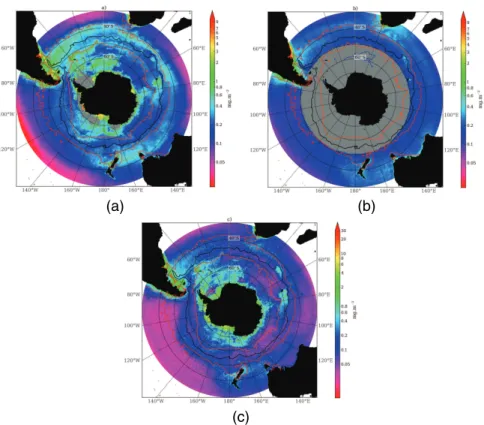
reflect a zonal (annular) character of variability such as observed between frontal and pelagic zones as well as remarkable regional contrasts between the Atlantic and Pa-cific Oceans (Fig. 1a). These spatial zones also display important seasonal contrasts and inter-annual variability (Fig. 1a–c). While technically an estimate of pigment con-centrations, we use SeaWiFS surface chlorophyll as a proxy for phytoplankton biomass

10

(Sullivan et al., 1993; Comiso et al., 1993; Moore et al., 1999; Moore and Abbott, 2000, 2002). Satellite surface chlorophyll concentrations do not however take into account deep chlorophyll maxima or changes in the carbon to chlorophyll ratio (C : Chl-a) with depth. Although typical deep chlorophyll maxima in the subtropics may result in un-derestimated satellite derived chlorophyll, typical chlorophyll profiles in the Southern

15

Ocean are uniform in the upper mixed layer and decreases exponentially at greater depths (Arrigo et al., 2008). The lack of depth integrated chlorophyll distribution is thus unlikely to significantly e_ffect satellite derived chlorophyll concentrations in the Southern Ocean. Changes in C : Chl-a are associated with physiological responses to changing light, temperature and nutrient conditions and are lowest at high

temper-20

atures (25–30◦_{C), low irradiances (}_<_{20 µmol photons m}−2_S−1_{) and nutrient replete} conditions and increase at high irradiances, low temperature and nutrient limiting con-ditions (Taylor et al., 1997). Although seasonal variability in C : Chl-aratios is significant at lower latitudes, the variations are relatively minor at higher latitudes when compared with the much larger seasonal range in chlorophyll concentration (Taylor et al., 1997).

25

(10)

sur-BGD

8, 4763–4804, 2011

Southern Ocean

Title Page

Tables Figures

◭ ◮

Back Close

Full Screen / Esc

Discussion

P

a

per

|

Dis

cussion

P

a

per

|

Discussion

P

a

per

|

Discussio

n

P

a

per

face chlorophyll measurements as a proxy for biomass, existing data suggest that these intra-cellular C : Chl-a ratios do not play a significant role in the seasonal cycle in the Southern Ocean (Taylor et al., 1997). In addition, standard ocean colour algorithms typically underestimate chlorophyll in the Southern Ocean by 2–3 times compared to in situ measurements (Kahru and Mitchell, 2010). Underestimated chlorophyll

concentra-5

tions are however unlikely to impact the characterisation of the patterns of the seasonal cycle which forms the primary focus of this paper.

In the subtropics, surface chlorophyll concentrations are low year round, except for a band of increased chlorophyll between 30◦ _{and 40}◦_{S in winter when nutrients are} replenished (Fig. 1b). Surface chlorophyll concentrations in the Southern Ocean are

10

low during the austral winter when light levels are low (Fig. 1b) (Mitchell et al., 1991; Veth et al., 1997; Lancelot et al., 2000; Smith et al., 2000; Boyd et al., 2001). Given the importance of Fe for photo-adaptation, Fe-light co-limitation is also likely (Sunda and Huntsman, 1997; Smith et al., 2000; Boyd et al., 2001). With the onset of a higher irradiance-mixing regime in spring, chlorophyll concentrations increase rapidly forming

15

blooms (Fig. 1a). Basin-scale differences are also evident with chlorophyll concentra-tions in the Pacific being noticeably lower than the Atlantic and Indian, in particular in the zonal band of 40–50◦_{S which disrupts the almost symmetrical distribution around} Antarctica. This band shows very little seasonal difference between summer and winter chlorophyll concentrations (Fig. 1a and b).

20

Lowest summer chlorophyll concentrations are associated with the pelagic waters north of the sea ice zone (Fig. 1a) where production rates are limited by deep mixing of the upper mixed layer and trace metal limitation (Mitchell and Holm-Hansen, 1991; Boyd et al., 2000; Sokolov and Rintoul, 2007a). An exception to these low production waters is found at oceanic frontal zones (Fig. 1a). Enhanced chlorophyll

concentra-25

(11)

BGD

8, 4763–4804, 2011

Southern Ocean

Title Page

Tables Figures

◭ ◮

Back Close

Full Screen / Esc

Discussion

P

a

per

|

Dis

cussion

P

a

per

|

Discussion

P

a

per

|

Discussio

n

P

a

per

|

(e.g., Lutjerharms et al., 1985; Perissinotto et al., 1992; Pollard and Regier et al., 1992; Laubscher et al., 1993; De Baar et al., 1995; Moore et al., 1999; Moore and Abbott, 2002). Although traditionally, enhanced chlorophyll concentrations have been associ-ated with mesoscale activities at the position of the fronts, Sokolov and Rintoul (2007b) more recently revealed that multiple frontal branches delimit regions with similar

el-5

evated chlorophyll concentrations and seasonality rather than the fronts themselves being associated with enhanced productivity, at least where fronts are distant from topography.

Another exception to low production Southern Ocean waters is found over regions of shallow bathymetry; around and downstream of subantarctic islands, over mid-ocean

10

ridges and large plateaus (Fig. 1a). In these regions of shallow bathymetry, current flow through relative vorticity (Hogg and Blundell, 2006; Moore et al., 1999) and/or bottom pressure torque (Sokolov and Rintoul, 2007a) is thought to increases the flux of Fe into surface waters (Korb and Whitehouse, 2004; Park et al., 2010; Venables and Mered-ith, 2010; Venables and Moore, 2010) accounting for the generally inverse correlation

15

between depth and chlorophyll in the Southern Ocean (Comiso et al., 1993). Highest chlorophyll concentrations are generally associated with the marginal ice zone (MIZ) and the continental shelf (Fig. 1a) (Smith and Gordon, 1997; Moore and Abbott, 2000; Arrigo and Van Dijken, 2004), through enhanced irradiance from increased vertical stratification when ice melts (Smith and Nelson, 1986), through Fe input from melting

20

ice (Sedwick and DiTullio, 1997; Gao et al., 2003; Grotti et al., 2005) and mixing of Fe rich sediments along the continental shelf (Schoemann et al., 1998; Johnson et al., 1999).

3.2 The seasonal cycle of chlorophyll in the Southern Ocean

The characteristics of the seasonal cycle of phytoplankton biomass in the Southern

25

(12)

BGD

8, 4763–4804, 2011

Southern Ocean

Title Page

Tables Figures

◭ ◮

Back Close

Full Screen / Esc

Discussion

P

a

per

|

Dis

cussion

P

a

per

|

Discussion

P

a

per

|

Discussio

n

P

a

per

is subsequently defined to four zonal regions. The subtropical zone (STZ), the transi-tion zone (TZ), the Antarctic circumpolar zone (ACZ) and the marginal ice zone (MIZ). The following section will describe the foundation for these zonal definitions based on seasonal characteristics rather than the distribution of chlorophyll concentrations, which has generally been the case in previous Southern Ocean studies. Defining the

5

Southern Ocean according to the characteristics of its seasonal cycle provides a more dynamic understanding of the characterisation of production based on underlying phys-ical drivers rather than climatologphys-ical biomass.

The chlorophyll bloom is considered a key phase in the seasonal cycle of phyto-plankton biomass. The circumpolar mean bloom initiation dates are depicted in Fig. 2.

10

Unlike in the Arctic, where significant trends towards earlier blooms were detected in 11 % of the area of the Arctic Ocean (Kahru et al., 2010), no homogenous regions showing distinct trends in either earlier or later bloom initiation dates were detected in the Southern Ocean, thus justifying the use of a 9 yr mean. In this study, the bloom initiation date has been associated with high biomass standing stocks and classified

15

statistically according to an increase in chlorophyll concentration relative to the an-nual median (Henson and Thomas, 2007; Follows and Dutkiewicz, 2002; Siegel et al., 2002). This classification of a phytoplankton bloom is different to that of a recent study by Behrenfeld (2010), which classifies the bloom initiation according to the time when phytoplankton population net growth rate becomes positive (see also Boss and

Behren-20

feld, 2010). Their results, based on chlorophyll concentrations in the North Atlantic, found that bloom initiation occurred in mid-winter when light levels are minimal and near-surface mixing is deepest. Behrenfeld’s dilution-recoupling hypothesis challenges Sverdrup’s Critical Depth Hypothesis (Sverdrup, 1953) by de-emphasizing the role of light and instead suggests a much greater role for the balance between

phytoplank-25

(13)

BGD

8, 4763–4804, 2011

Southern Ocean

Title Page

Tables Figures

◭ ◮

Back Close

Full Screen / Esc

Discussion

P

a

per

|

Dis

cussion

P

a

per

|

Discussion

P

a

per

|

Discussio

n

P

a

per

|

in phytoplankton productivity, CO₂uptake and carbon export, all of which are products of phytoplankton biomass and specific growth rates (Boss and Behrenfeld, 2010). The annual cycles of phytoplankton biomass in our results emphasize the role of bottom-up controls (light and nutrients) on increases in phytoplankton specific growth rates for determining bloom initiation (Sverdrup, 1953). The lack of information on growth

5

rates does not allow us to quantify the role of grazing. In this study, we do not assume that the role of grazing is negligible, but rather that statistically significant seasonal in-creases in biomass can only occur when specific growth rates exceed loss terms and net population growth remains positive, despite potential increases in grazing pressure associated with increased encounter rates when the seasonal mixed layer shallows.

10

According to Fig. 2, bloom initiation in the STZ (∼30–40◦S), is characterized by an

onset taking place in autumn (April–June) when macro-nutrients are replenished with the deepening of the seasonal mixed layer. This STZ is well defined in its latitudinal extent. North of∼30◦S, insufficient heat loss in winter limits the breakdown of

stratifi-cation and deep winter overturning to below the nutricline preventing winter increases

15

in chlorophyll biomass. South of∼40◦S, low winter PAR limits net primary productivity,

preventing concomitant increases in winter chlorophyll concentrations, forcing phyto-plankton populations towards spring bloom initiations (September–November). The transition between autumn and spring bloom initiations is remarkably abrupt (with the exception of the central and eastern Pacific where the transition is extended in latitude).

20

The abrupt transition is indicative of a rapid shift from one seasonal regime to another, rather than a monotonic progression in the timing of the bloom initiation with increasing latitude. Further south is the MIZ where bloom initiation dates are in summer (Decem-ber to February), reflecting the delay in seasonal PAR availability as well as the time it takes for phytoplankton blooms to fully respond to the newly created ice-free waters

25

associated with the region (Arrigo et al., 2008).

(14)

BGD

8, 4763–4804, 2011

Southern Ocean

Title Page

Tables Figures

◭ ◮

Back Close

Full Screen / Esc

Discussion

P

a

per

|

Dis

cussion

P

a

per

|

Discussion

P

a

per

|

Discussio

n

P

a

per

of Tasmania, ∼42◦S, 147◦E). The transition between zonally comparable regions of

early and late bloom onset can be relatively abrupt: for example the region of early (September, 100–140◦_{E) and late (December, 130–170}◦_{E) bloom development found} south of Australia (50–55◦_{S) and the region of early onset evident north east of Crozet} where the spring bloom starts particularly early in the year (May).

5

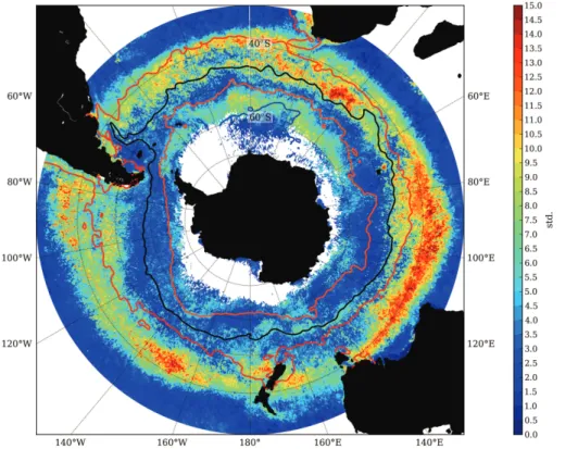
Regions with high inter-annual variability (std. dev. 10–16) in bloom initiation date (Fig. 3) correspond to transition regions between di_fferent seasonal regimes. In par-ticular the transition between autumn and spring bloom initiation around∼40◦S. The

boundaries of this region of high variability in bloom initiation define what we term the TZ. The remaining region of spring bloom initiation between the TZ and MIZ is what

10

we term the ACZ. Other regions of high variability in bloom initiation similarly coin-cide with transition regions between different seasonal regimes, e.g. the region of late bloom initiation south of Australia (130–170◦_{E) and the transition between spring and} summer bloom initiation at the confluence of the ACZ and MIZ which is particularly extended in the Atlantic and the western Indian Ocean sector (20◦_W–60◦_{E). Although}

15

the shift in mean bloom initiation date appears abrupt (Fig. 2), the TZ of high variability in bloom initiation dates is extended in latitude highlighting the discrepancy between climatological (Fig. 2) and annual time series (Fig. 3).

The percentage of the variance explained by the mean seasonal cycle (Fig. 4) de-fines how well the mean climatological seasonal cycle (from 9 yr) represents the

evolu-20

tion of chlorophyll over each year. Immediately apparent from this figure are the sharp gradients between strongly contrasting regions where the seasonal cycle for each year is coherent with the 9 yr mean (i.e. high seasonality; >70 %) compared to regions where there is large variability from year to year in the timing and amplitude of the bloom and only a low percentage of the variance is explained by the mean seasonal

25

cycle (i.e. low seasonality;<30 %) (Fig. 4).

Despite the amplitude of the seasonal cycle in the STZ being weak (∼0 to

(15)

BGD

8, 4763–4804, 2011

Southern Ocean

Title Page

Tables Figures

◭ ◮

Back Close

Full Screen / Esc

Discussion

P

a

per

|

Dis

cussion

P

a

per

|

Discussion

P

a

per

|

Discussio

n

P

a

per

|

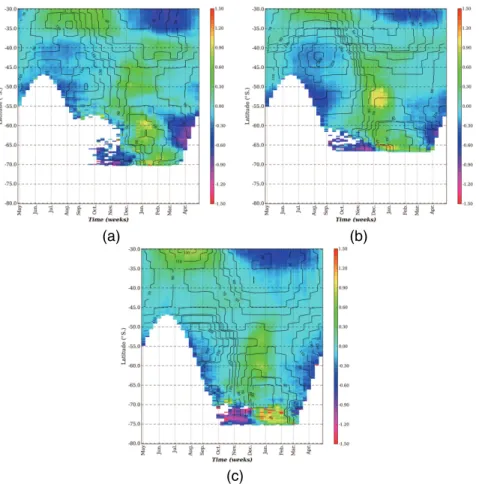
cycle (>70 % of variance explained) (Fig. 4). An example of the time series of chloro-phyll compared to the climatological mean seasonal in the STZ is shown in Fig. 5a. In this nutrient limited region, phytoplankton blooms occur in a predictable manner (std. dev. <4, Fig. 3; R2₌91, Fig. 5a) when seasonal net heat loss and overturning in late autumn/early winter deepens the mixed layer to below the nutricline, relieving

nu-5

trient stress in surface waters and allowing phytoplankton production and biomass to increase. This finding agrees well with Dandonneau et al. (2004), who found low ratios of inter-annual to total variance from monthly SeaWiFS chlorophyll concentrations in the subtropical band between 1998 and 2001.

In the ACZ and MIZ, large regions of relatively high seasonality are also found, e.g.

10

in the Pacific south of 50◦_{S (}

∼50 %), east of Kerguellen (∼49◦S, 70◦E) (60–80 %) and

a finer scale banded structure associated with the SAF zone and PF zone in the east-ern Atlantic (50–70◦_{S, 0–10}◦_{E) (Fig. 4). In regions with a high degree of seasonality} (e.g. Fig. 5b and c;R2₌66 and 64, respectively) one would expect that intra-seasonal forcing does not play a significant role in the phytoplankton seasonal cycle and that

15

the annual time series would be almost entirely explained by the seasonal forcing of light, heat flux and seasonal MLD (as in the subtropics, e.g. Fig. 5a). This does not mean that Fe or light is not limiting but merely that it does not vary sufficiently on an intra-seasonal time scale to influence the inter-annual variability of the phytoplank-ton seasonal expression. In such instances one would expect there to be sufficient

20

winter preconditioning of the water column with limiting nutrients (notably Fe) to allow a bloom initiation when the seasonal PAR threshold for increased primary production and biomass accumulation is met in spring. The amplitude of the seasonal bloom would depend on the supply of Fe via physical forcing mechanisms that include a) the seasonal re-supply of Fe through winter overturning, b) the depth of the summer

25

(16)

BGD

8, 4763–4804, 2011

Southern Ocean

Title Page

Tables Figures

◭ ◮

Back Close

Full Screen / Esc

Discussion

P

a

per

|

Dis

cussion

P

a

per

|

Discussion

P

a

per

|

Discussio

n

P

a

per

blooms, respectively). In these instances, the intra-seasonal re-supply of Fe to surface waters through wind mixing or mesoscale variability plays a less significant role in pro-moting phytoplankton growth, hence the low degree of intra-seasonal and inter-annual variability (R2₌66 andR2₌66, Fig. 5b and c, respectively).

Regions of low seasonality (Fig. 4) generally correspond to regions of high

variabil-5

ity in the phasing of the bloom initiation (Fig. 3). The zone of low variance explained by the mean seasonal cycle (<20 %) marks the TZ (∼40◦S). This region is

partic-ularly extensive in the Pacific (∼40–50◦S), where chlorophyll concentrations are so

low that the seasonal cycle is indistinguishable from intra-seasonal noise (e.g. Fig. 5d; R2₌27). The transition between spring and summer bloom initiation at the ACZ and

10

MIZ confluence also marks a region of low seasonality. At a smaller scale, transitions between regions of contrasting bloom initiation dates within the ACZ are also charac-terized by weak seasonality e.g. the region of low variance explained by the seasonal cycle corresponding to the region of late bloom initiation south of Australia.

Low seasonality related to the transition between regions of different bloom initiation

15

is potentially related to the diversity of conditions encountered at the confluence be-tween contrasting seasonal regimes. Transition regions of low seasonality are thought to be driven by a combination of multiple limiting factors and forcing mechanisms from both seasonal regimes. If there are too many factors simultaneously limiting phyto-plankton production (e.g. nutrients and light), phytophyto-plankton are not able to optimise to

20

their environment, restricting the ability of the system to build up biomass. The expres-sion of this will manifest as low annual chlorophyll concentrations with high inter-annual and intra-seasonal variability in bloom characteristics such as are found at the TZ in the Pacific (Figs. 4 and 5d).

Low seasonality (Fig. 4) does not however necessarily coincide with low

chloro-25

phyll concentrations (Fig. 1a). The TZ of low seasonality in the Atlantic and Indian has relatively high summer chlorophyll concentrations (e.g. Fig. 5e; R2₌44; chloro-phyll max=∼1 mg m−3). Likewise, low seasonality regions surrounding the

(17)

BGD

8, 4763–4804, 2011

Southern Ocean

Title Page

Tables Figures

◭ ◮

Back Close

Full Screen / Esc

Discussion

P

a

per

|

Dis

cussion

P

a

per

|

Discussion

P

a

per

|

Discussio

n

P

a

per

|

concentrations (Fig. 1a). If our hypothesis for the low chlorophyll concentrations in the Pacific TZ holds true then there has to be a reduction in the number of factors simul-taneously limiting production in regions of low seasonality but high chlorophyll. We propose that in these regions intra-seasonal physical forcing mechanisms are sequen-tially relieving light and/or nutrients at a frequency that is long enough to allow

phyto-5

plankton blooms to fully develop. At the latitudes of the continental margins of Africa and America for example, nutrients rather than light are considered the dominant lim-iting factor in summer. The upwelling of nutrients, particularly on eastern boundaries, through periodic wind events relieves nutrient stress on a sub-seasonal time scale. The period of sub-seasonal forcing must optimise growth in biomass at rates that

ex-10

ceed losses to account for the high integrated summer chlorophyll concentrations found here. The sub-seasonal wind events responsible for the upwelling and mixing of nutri-ents are likely to be responsible for the high intra-seasonal and inter-annual variability expressed as low seasonality. Along the continental margins of Antarctica on the other hand, elevated Fe associated with the continental shelf and ice melt (Fitch and Moore,

15

2007) makes light the dominant limiting factor. Intra-seasonal forcing of the interac-tion between a deepening of the MLD through wind mixing and the re-establishment of stratification through fresh water buoyancy, at adequate time scales, similarly accounts for the high chlorophyll concentrations but low seasonality found in this region.

The Supplement accompanying Figs. S1–4 elaborates on intra-seasonal and

inter-20

annual variability (that result in either high or low seasonality) and complements the zonal characterisation of the Southern Ocean’s seasonal cycle. Inter-annual and intra-seasonal variability in the STZ is low and consistent with a high degree of intra-seasonality (Fig. 4), whereas in the TZ, inter-annual and intra-seasonal variability is particularly high and seasonality consequently weak. A well defined but short lived bloom is found

25

(18)

BGD

8, 4763–4804, 2011

Southern Ocean

Title Page

Tables Figures

◭ ◮

Back Close

Full Screen / Esc

Discussion

P

a

per

|

Dis

cussion

P

a

per

|

Discussion

P

a

per

|

Discussio

n

P

a

per

Although the fronts of the STF and ACC clearly influence the regional characterisa-tion of the seasonal cycle of chlorophyll in the Southern Ocean (Figs. 1a, 2, 4), the physical forcing mechanisms responsible for enhanced chlorophyll (large scale flow versus small scale instabilities) are still unclear and need to be investigated further. Sokolov and Rintoul (2007) propose that mean chlorophyll distribution (and seasonal

5

cycle) is best explained by upwelling where the ACC interacts with topography, fol-lowed by downstream advection where flow-topography interactions drive upwelling of nutrients, independent of mesoscale instabilities. Fronts however are known to provide a source of buoyancy through mesoscale and sub-mesoscale instabilities which influ-ence phytoplankton production through nutrient supply (upwelling) and light availability

10

(stratification) (Swart and Speich, 2010; Kahru et al., 2007) as well as being zones of seasonal convergence. High resolution satellite imagery and model simulations now show that incorrect representation of sub-mesoscale frontogenesis can result in er-rors of up to 50 % in primary production estimates (Levy et al., 2001; Glover et al., 2008). Despite the significant contribution of fronts to characterising both the spatial

15

and seasonal distribution of chlorophyll in the Southern Ocean, the contrasting view points in the literature highlights the indeterminate role of the fronts in controlling phy-toplankton production. These differences seem to depend on the light/Fe co-limitation regime that they are superimposed upon which in effect determines the physical forcing mechanism that is ultimately responsible for the observed variability in the chlorophyll

20

seasonal cycle.

3.3 Mixed layer depth, irradiance and the phytoplankton seasonal cycle

As expected, mean MLD’s for winter (August) are deeper than in summer (February) and present large spatial variability (Fig. 6a and b). In the Atlantic (∼20◦E–20◦W)

and eastern Indian Ocean (∼60–180◦E), MLD’s of >200 and >300 m respectively 25

are found between∼40 and 50◦S in winter (Fig. 6a). Whereas in the Pacific in

win-ter, (∼150–70◦W) MLD’s of >400 m are found further south between∼50 and 60◦S.

In the 40–50◦_{S latitudinal band, MLD’s are relatively shallow (}

(19)

BGD

8, 4763–4804, 2011

Southern Ocean

Title Page

Tables Figures

◭ ◮

Back Close

Full Screen / Esc

Discussion

P

a

per

|

Dis

cussion

P

a

per

|

Discussion

P

a

per

|

Discussio

n

P

a

per

|

compared to similar latitudes in the Atlantic and Indian (Fig. 6a). MLD’s in summer present a more zonally coherent distribution, with MLD’s shallower than ∼50 m

ob-served north of 40◦_{S and south of 60}◦_{S, with MLD’s of 80–120 m in between (Fig. 6b).} The chlorophyll concentration at the sea surface generally responds to the seasonal cycle of solar radiation which strongly impacts vertical stability through net heat flux,

in-5

fluencing vertical nutrient supply and the timing and intensity of phytoplankton blooms (Dandonneau et al., 2004). A first order estimate of the large-scale relationship be-tween the seasonal cycles of MLD and chlorophyll (Fig. 7) can therefore be used to improve our understanding of the transition between different seasonal regimes.

Consistent with our understanding of the subtropics as a nutrient-limited regime, the

10

correlation in the STZ is uniformly positive (>0.8), with increased chlorophyll associ-ated with of the deepest winter MLD’s. High chlorophyll concentrations coinciding with deep MLD’s in the subtropics are likely enhanced by photoadaptation of light limited cells in the deep winter mixed layer (Letelier et al., 1993).

The transition between a positive and negative correlation (Fig. 7) corresponds

re-15

markably well to the transition between winter and summer centred seasonal cycles (Fig. 2) reflecting the sharp climatological change in physical control mechanisms. Negative correlations are evident in the ACZ and MIZ, consistent with a light lim-ited regime where increased chlorophyll concentrations coincide with shallow MLD’s. A shoaling of the MLD provides the required light environment for phytoplankton

pro-20

duction favouring increases in specific growth rates that exceeds export and losses through grazing and results in biomass accumulation (Sverdrup, 1953; Mitchell et al., 1991a; Comiso et al., 1993). However, in these high latitudes, low light (PAR) envi-ronments, the relationship is more convoluted than in the subtropics, with areas of low and in some instances slightly positive correlations (e.g., Crozet) interspersed among

25

(20)

BGD

8, 4763–4804, 2011

Southern Ocean

Title Page

Tables Figures

◭ ◮

Back Close

Full Screen / Esc

Discussion

P

a

per

|

Dis

cussion

P

a

per

|

Discussion

P

a

per

|

Discussio

n

P

a

per

dynamics in the Southern Ocean are more varied and complex, as are the require-ments to promote phytoplankton growth. Although the prevailing negative correlation between MLD and surface chlorophyll suggests that light is more important in limit-ing production in the subantarctic (relative to the subtropics), the Southern Ocean is also nutrient limited, in particular with regards to Fe and Si (Boyd et al., 2002). The

5

prolonged persistence of a shallow mixed layer can in some cases lead to nutrient limi-tation of primary production such that a periodic intra-seasonal deepening of the mixed layer (allowing Fe re-supply), at time scales of the same order as the phytoplankton growth rate, is necessary to maintain production rates at high levels throughout the summer season (Pasquero et al., 2005). In such instances, phytoplankton population

10

growth rates are able to exceed their losses resulting in a well defined seasonal phyto-plankton bloom (the integrated effect of localised sub-seasonal blooms) that does not coincide with the shallowest MLD’s.

Changes in the mixed layer result from the interaction of turbulent mixing, through wind stress, and buoyancy forcing, through air/sea heat fluxes, fresh water fluxes,

en-15

trainment and advection (geostrophic and Ekman). These two drivers (turbulent mixing and buoyancy forcing) compete to either strengthen stratification or destroy it. We propose that the complex nature of the controls on stratification and production in the Southern Ocean plays an instrumental role in the expression of seasonal, sub-seasonal and regional variability in chlorophyll concentrations and the sub-seasonal cycle.

20

3.4 Basin scale meridional controls of the seasonal cycle

The zonally asymmetric nature of the seasonal cycle of chlorophyll in the Southern Ocean provides the impetus for basin scale comparisons in addition to zonal charac-terisation. This asymmetry was similarly noted in the response of the MLD to the SAM by Salle et al. (2009). From a heat budget of the mixed layer they conclude that

merid-25

(21)

BGD

8, 4763–4804, 2011

Southern Ocean

Title Page

Tables Figures

◭ ◮

Back Close

Full Screen / Esc

Discussion

P

a

per

|

Dis

cussion

P

a

per

|

Discussion

P

a

per

|

Discussio

n

P

a

per

|

to more accurately characterise regional differences in the phasing of the chlorophyll bloom with respect to MLD’s. The seasonal progression of chlorophyll anomalies with respect to the annual mean were plotted with mean MLD’s for three transects, one in each of the ocean basins (Fig. 8a–c).

For each of the three transects a similar latitudinal progression in seasonal

char-5

acteristics of the chlorophyll bloom is evident (Fig. 8a–c). In the STZ to the north maximum chlorophyll concentrations are in winter spanning August to October in the Atlantic (Fig. 8a), July to September in the Indian (Fig. 8b) and June to September in the Pacific (Fig. 8c), coincident with maximum winter MLD’s (50–30 m). Minimum chloro-phyll concentrations occur in late summer (January to March) when MLD’s are shallow

10

(20–50 m). There is a southward extension of the STZ in the Pacific (∼30–40◦S)

rel-ative the Atlantic and Indian (∼30–35◦S). Further south, in the ACZ, the phasing of

the chlorophyll bloom switches to one in which maximum concentrations are centred around the summer months (November to January), following the shoaling of the winter mixed layer (<70 m). In the MIZ bloom initiation occurs one month later (Fig. 2) with

15

maximum concentrations extend into autumn (March) coinciding with shallowest MLD’s (30–40 m). The presence of the Weddell Gyre in the Atlantic transect (Fig. 8a) broad-ens the latitudinal extent of the MIZ (∼57–70◦S) compared to the Indian (∼60–65◦S)

and Pacific (∼70–75◦S) (Fig. 8b and c).

Besides the comparable characteristics in latitudinal progression of the seasonal

cy-20

cle, inter-ocean basin differences are also evident. The Atlantic and Indian transects (Fig. 8a and b) are characterised by a relatively rapid TZ (∼35–40◦S), the northern

boundary of the summer bloom region of the ACZ occurring at ∼37◦S and ∼43◦S,

respectively. In the Pacific transect (Fig. 8c); the TZ between winter and summer cen-tred seasonal regimes is extended in latitude to∼10 degrees (40–50◦S), with distinct 25

(22)

BGD

8, 4763–4804, 2011

Southern Ocean

Title Page

Tables Figures

◭ ◮

Back Close

Full Screen / Esc

Discussion

P

a

per

|

Dis

cussion

P

a

per

|

Discussion

P

a

per

|

Discussio

n

P

a

per

winter mixed layer in the 40–50◦_{S latitudinal band in the Pacific (90–100 m) is unclear} (see also Fig. 6a), it is likely that an additional sustained input of buoyancy (e.g. ad-ditional heat source from southward penetrations of subtropical water) prevents the deepening of the mixed layer in winter to depths comparable to those of the Atlantic and Indian (130 and 250 m, respectively).

5

Intuitively, the Pacific, when compared to the Atlantic and Indian, has a potentially lower Fe supply to surface waters through the lack of continental or subantarctic island and sub-ocean land mass and lower mesoscale eddy activity from a lack of bathymetry to interact with the mean flow. Increased eddy kinetic energy associated with such fea-tures, enhances the sub-surface flux of Fe into surface waters, potentially enhancing

10

phytoplankton growth (Hense et al., 2000; Moore et al., 1999; Sokolov and Rintoul, 2007a; Park et al., 2010). If the main source of Fe to the surface waters (73–99 %) of the Southern Ocean is through upwelling (Johnson et al., 1997; Lefevre and Watson, 1999; Archer and Johnson, 2000), one can deduce that in the Pacific, where Fe sup-ply to surface waters through deep water entrainment is limited, shallow winter mixed

15

layers are unlikely to be deep enough to entrain sufficient Fe into the surface waters for stimulating and maintaining high production rates through the summer. Hence, the extended (35–49◦_{S) low chlorophyll TZ in the Pacific, with high variability and low} sea-sonality likely results from Fe limitation.

4 Synthesis

20

Characterising the Southern Ocean according to the variability of the seasonal cy-cle provides a more dynamic understanding of the spatial heterogeneity of production based on underlying physical drivers rather than mean climatological biomass. Based on our analysis of the timing, variability and seasonality of seasonal chlorophyll distri-butions, we defined the spatial distribution of the seasonal cycle into four zonal regions:

25

(1) the STZ (∼30–35 or 40◦S), characterised by an autumn bloom initiation (Fig. 2),

(23)

BGD

8, 4763–4804, 2011

Southern Ocean

Title Page

Tables Figures

◭ ◮

Back Close

Full Screen / Esc

Discussion

P

a

per

|

Dis

cussion

P

a

per

|

Discussion

P

a

per

|

Discussio

n

P

a

per

|

of high variability in bloom initiation dates (centred around∼40◦S) (Fig. 3), where

inter-annual and intra-seasonal variability is also high and seasonality consequently weak (Fig. 4); (3) The ACZ (south of the TZ) where bloom initiations are generally in spring (Fig. 2), inter-annual variability in bloom initiation dates is low (Fig. 3) and large areas of both high and low seasonality are found (Fig. 4), and (4) The (MIZ) where bloom

5

initiations are in summer (Fig. 2), variability in bloom initiation dates is low (Fig. 3) but inter-annual and intra-seasonal variability in the chlorophyll seasonal cycle is high, leading to low seasonality (Fig. 4).

This zonal classification effectively characterises the variability of the seasonal cycle in the Southern Ocean. However, when the response of the biology to the underlying

10

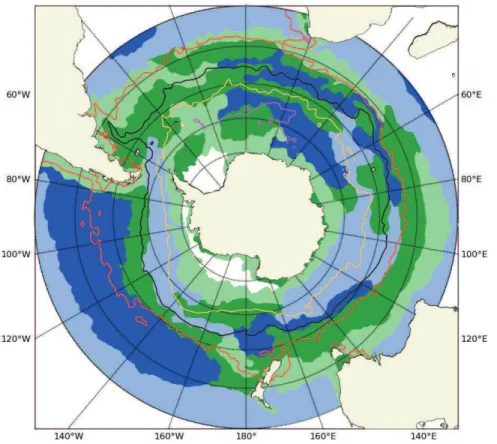
physics of the different seasonal regimes was taken into consideration (i.e. low versus high seasonal chlorophyll maxima), an additional classification system was required. In order to summarise the varying responses of the phytoplankton community to the different seasonal regimes, we created a schematic that divides the Southern Ocean into a montage of four regions in addition to the four seasonal zones (Fig. 9). This

15

schematic is created from a composite of the mean summer chlorophyll concentration from November to January (1998–2007) and the variance explained by the seasonal cycle (Fig. 4). The four regions result from a combination of high or low chlorophyll concentration and high or low seasonality. No allowance has been made for interme-diate chlorophyll concentrations or seasonality, and as a consequence the boundaries

20

between regions are not definitive. This needs to be taken into consideration when interpreting this figure which is intended as a support to a conceptual framework on the nature of the controls of variability in the phytoplankton seasonal cycle.

Region A is representative of a nutrient limited regime with low chlorophyll concen-trations but high seasonality. In Region A, in the STZ (30–40◦_{S), nutrients (in particular}

25

(24)

BGD

8, 4763–4804, 2011

Southern Ocean

Title Page

Tables Figures

◭ ◮

Back Close

Full Screen / Esc

Discussion

P

a

per

|

Dis

cussion

P

a

per

|

Discussion

P

a

per

|

Discussio

n

P

a

per

topographic features) is also nutrient limited. Winter overturning re-supplies limiting surface nutrients (in particular Fe) to support an increase in phytoplankton growth, but only in spring when light levels are sufficient. In these regions, the available nutrients are rapidly used up by the phytoplankton community and the bloom subsequently de-clines when community losses outweigh growth rates. Despite the amplitude of the

5

seasonal cycle in these regions being weak, the overall variability of the chlorophyll signal is strongly phase-locked to the annual seasonal cycle. In these regions, no sub-seasonal forcing of the mixed layer to below the nutricline is replenishing surface nutrients on intra-seasonal time scales, which accounts for the low intra-seasonal and inter-annual variability and a predictable seasonal cycle (high seasonality).

10

The second region with low chlorophyll concentrations (Region B) is also charac-terised by low Fe concentrations but this region displays low seasonality. This region is particularly extensive in the Pacific where increased positive buoyancy forcing po-tentially prevents the deepening of the winter mixed layer to below the ferricline, thus failing to re-set the seasonal Fe supply. If the winter re-supply of Fe to surface waters

15

is insufficient and/or the depth of the ferricline is below the deepest summer MLD’s then phytoplankton lack the potential to significantly increase their biomass during the summer season through Fe limitation. These regions are characterised by chlorophyll concentrations that are so low and intra-seasonal variability so high that the seasonal cycle is indistinguishable from intra-seasonal noise.

20

The last two regions refer to areas of high chlorophyll but with either a low (Region C) or high (Region D) seasonality. Regions of high chlorophyll in the Southern Ocean result from integrated seasonal primary production that exceeds community losses and according to the literature results from the relief of Fe stress at ocean fronts, over shallow bathymetry, along continental margins and in the MIZ (e.g., Boyd et al., 2002).

25

The different seasonal expressions of high and low seasonality, however implies distinct physical supply mechanisms of Fe and light to the surface waters.

(25)

BGD

8, 4763–4804, 2011

Southern Ocean

Title Page

Tables Figures

◭ ◮

Back Close

Full Screen / Esc

Discussion

P

a

per

|

Dis

cussion

P

a

per

|

Discussion

P

a

per

|

Discussio

n

P

a

per

|

summer chlorophyll. In these regions, the annual time series is almost entirely ex-plained by the seasonal forcing of light, heat flux and seasonal MLD (as in the subtrop-ics). This is not to say that Fe or light is not a limiting factor but merely that it does not vary sufficiently on an intra-seasonal time scale to influence the inter-annual variability of the phytoplankton seasonal expression. In such instances sufficient winter

precon-5

ditioning of the water column with limiting nutrients is required in order to allow a spring bloom initiation. The integrated seasonal amplitude of the bloom would depend on the amount of Fe made available through winter overturning, the depth of the summer mixed layer relative to the nutricline, lateral advection of Fe into surface waters and upwelling at fronts.

10

In regions of high chlorophyll but low seasonality (Region D), the seasonal character-istics of high inter-annual and intra-seasonal variability are controlled by sub-seasonal forcing of the nutrient and light supply. In these regions, we hypothesize that high integrated summer chlorophyll concentrations are a direct consequence of high intra-seasonal physical forcing of the MLD at appropriate time scales (Pasquero et al., 2005).

15

In these regions, shallow MLD’s likely lead to short term depletions of surface nutrients such that a periodic deepening of the ML (to below the nutricline) is necessary for phy-toplankton population growth to occur. This high intra-seasonal variability culminates from a combination of high wind stress variability at appropriate time scales and upper water column stabilisation through positive buoyancy forcing via mesoscale dynamics

20

and fresh water (ice melt) fluxes.

Although the fronts of the STF and ACC clearly influence the regional characterisa-tion of the seasonal cycle of chlorophyll in the Southern Ocean, the physical forcing mechanisms responsible for enhanced chlorophyll (large scale flow versus small scale instabilities) are still unclear and need to be investigated further.

25

(26)

BGD

8, 4763–4804, 2011

Southern Ocean

Title Page

Tables Figures

◭ ◮

Back Close

Full Screen / Esc

Discussion

P

a

per

|

Dis

cussion

P

a

per

|

Discussion

P

a

per

|

Discussio

n

P

a

per

through changes in the characteristics of the seasonal cycle. A better understanding of the regional sensitivities of the Southern Oceans biological pump to climate change will allow us to make more robust predictions of long term trends.

Supplementary material related to this article is available online at: http://www.biogeosciences-discuss.net/8/4763/2011/

5

bgd-8-4763-2011-supplement.pdf.

Acknowledgements. This work was undertaken and supported through the Southern Ocean Carbon – Climate Observatory (SOCCO) Programme. S. J. Thomalla and S. Swart were supported through SOCCO post doctoral fellowships funded by ACCESS and NRF/SANAP. P. M. S. Monteiro and N. Fauchereau were supported by CSIR’s Parliamentary Grant.

10

References

Archer, D. E. and Johnson, K.: A model of the iron cycle in the ocean, Global Biogeochem. Cy., 14, 269–279, 2000.

Arrigo, K. R. and van Dijken, G. L.: Annual changes in sea-ice, chlorophyll a, and primary production in the Ross Sea, Antarctica, Deep-Sea Res. Pt. II, 51, 117–138, 2004.

15

Arrigo, K. R., van Dijken, G. L., and Bushinsky, S.: Primary production in the Southern Ocean, 1997–2006, J. Geophys. Res., 113, C08004, doi:10.1029/2007JC004551, 2008.

Banse, K.: Low seasonality of low concentrations of surface chlorophyll in the Subantarctic water ring: underwater irradiance, iron or grazing?, Prog. Oceanogr., 37, 241–91, 1996. Behrenfeld, M. J.: Abandoning Sverdrup’s critical depth hypothesis, Ecology, 91, 977–989,

20

doi:10.1890/09-1207.1, 2010.

Blain, S., Queguiner, B., Armand, L., Belviso, S., Bombled, B., Bopp, L., Bowie, A., Brunet, C., Brussaard, C., Carlotti, F., Christaki, U., Corbiere, A., Durand, I., Ebersbach, F., Fuda, J., Gar-cia, N., Gerringa, L., Griffiths, B., Guigue, C., Guillerm, C., Jacquet, S., Jeandel, C., Laan, P., Lefevre, D., Lo Monaco, C., Malits, A., Mosseri, J., Obernosterer, I., Park, Y., Picheral, M.,

25

(27)

Vin-BGD

8, 4763–4804, 2011

Southern Ocean

Title Page

Tables Figures

◭ ◮

Back Close

Full Screen / Esc

Discussion

P

a

per

|

Dis

cussion

P

a

per

|

Discussion

P

a

per

|

Discussio

n

P

a

per

|

cent, D., Viollier, E., Vong, L., and Wagener, T.: Effect of natural iron fertilization on carbon sequestration in the Southern Ocean, Nature, 446, 1070–1074, 2007.

B ¨oning, C. W., Dispert, A., Visbeck, M., Rintoul, S. R., and Schwarzkopf, F.: The response of the Antarctic Circumpolar Current to recent climate change, Nat. Geosci., 1, 864–869, 2008. Boss, E. and Behernfeld, M.: In situ evaluation of the initiation of the North Atlantic

phytoplank-5

ton bloom, Geophys. Res. Lett., 37, L18603, doi:10.1029/2010GL044174, 2010.

Boyd, P. W.: Environmental factors controlling phytoplankton processes in the Southern Ocean, J. Phycol., 38, 844–861, 2002.

Boyd, P. W., Watson, A., Law, C. S., Abraham, E., Trull, T., Murdoch, R., Bakker, D. C. E., Bowie, A. R., Charette, M., Croot, P., Downing, K., Frew, R., Gall, M., Hadfield, M., Hall, J.,

10

Harvey, M., Jameson, G., La Roche, J., Liddicoat, M., Ling, R., Maldonado, M., McKay, R. M., Nodder, S., Pickmere, S., Pridmore, R., Rintoul, S., Safi, K., Sutton, P., Strzepek, R., Tan-neberger, K., Turner, S., Waite, A., and Zeldis, J.: A mesoscale phytoplankton bloom in the polar Southern Ocean stimulated by iron fertilization, Nature, 407, 695–702, 2000.

Boyd, P. W., Crossley, A. C., DiTullio, G. R., Griffiths, F. B., Hutchins, D. A., Queguiner, B.,

15

Sedwick, P. N., and Trull., T. W.: Effects of iron supply and irradiance on phytoplankton processes in subantarctic waters south of Australia, J. Geophys. Res., 106, 31573–31584, 2001.

de Boyer Mont ´egut, C., Madec, G., Fischer, A. S., Lazar, A., and Iudicone, D.: Mixed layer depth over the global ocean: an examination of profile data and a profile-based climatology,

20

J. Geophys. Res., 109, C12003, doi:10.1029/2004JC002378, 2004.

Caldeira, K. and Duffy P. B.: The role of the Southern Ocean in uptake and storage of anthro-pogenic carbon dioxide, Science, 87, 620–622, doi:10.1126/Science. 287.5453.620, 2000. Campbell, J. W.: The lognormal distribution as a model for bio-optical variability in the sea, J.

Geophys. Res., 100, 13237–13254, 1995.

25

Campbell, J. W. and Aarup, T.: Photosynthetically available radiation at high latitudes, Limnol. Oceanogr., 34, 1490–1499, 1989.

Comiso, J. C., McClain, C. R., Sullivan, C. W., Ryan, J. P., and Leonard, C. L.: Coastal zone color scanner pigment concentrations in the Southern Ocean and relationships to geophysi-cal surface features, J. Geophys. Res., 98, 2419–2451, 1993.

30

Cullen, J. J.: Hypotheses to explain high-nutrient conditions in the open sea, Limnol. Oceanogr., 36, 1578–1599, 1991.