www.biogeosciences.net/8/2849/2011/ doi:10.5194/bg-8-2849-2011
© Author(s) 2011. CC Attribution 3.0 License.
Biogeosciences
Regional scale characteristics of the seasonal cycle
of chlorophyll in the Southern Ocean
S. J. Thomalla1,2, N. Fauchereau1, S. Swart1,2, and P. M. S. Monteiro1
1Ocean Systems and Climate Group, CSIR, P.O. Box 320, Stellenbosch, 7599, South Africa 2Department of Oceanography, UCT, Private Bag, Rondebosch, 7700, South Africa Received: 2 February 2011 – Published in Biogeosciences Discuss.: 13 May 2011
Revised: 15 September 2011 – Accepted: 15 September 2011 – Published: 7 October 2011
Abstract. In the Ocean, the seasonal cycle is the mode that
couples climate forcing to ecosystem response in production, diversity and carbon export. A better characterisation of the ecosystem’s seasonal cycle therefore addresses an important gap in our ability to estimate the sensitivity of the biological pump to climate change. In this study, the regional charac-teristics of the seasonal cycle of phytoplankton biomass in the Southern Ocean are examined in terms of the timing of the bloom initiation, its amplitude, regional scale variabil-ity and the importance of the climatological seasonal cycle in explaining the overall variance. The seasonal cycle was consequently defined into four broad zonal regions; the sub-tropical zone (STZ), the transition zone (TZ), the Antarctic circumpolar zone (ACZ) and the marginal ice zone (MIZ). Defining the Southern Ocean according to the characteristics of its seasonal cycle provides a more dynamic understanding of ocean productivity based on underlying physical drivers rather than climatological biomass. The response of the biol-ogy to the underlying physics of the different seasonal zones resulted in an additional classification of four regions based on the extent of inter-annual seasonal phase locking and the magnitude of the integrated seasonal biomass. This regional-isation contributes towards an improved understanding of the regional differences in the sensitivity of the Southern Oceans ecosystem to climate forcing, potentially allowing more ro-bust predictions of the effects of long term climate trends.
1 Introduction
Biological production and carbon export to the deep ocean, “the biological pump” is considered a major contributor to the Southern Ocean CO2sink removing an estimated 3 PgC
Correspondence to:S. J. Thomalla (sandy.thomalla@gmail.com)
(1 PgC = 1015g of carbon) from surface waters south of 30◦S
each year (33 % of the global organic carbon flux) (Schlitzer, 2002). The Southern Ocean biological pump also plays an important role in regulating the supply of nutrients to ther-mocline waters (Subantarctic Mode Water and Intermediate Water) of the entire Southern Hemisphere and North Atlantic (Sarmiento et al., 2004), which in turn drives low latitude productivity (Sigman and Boyle, 2000). Climate models and decadal data sets suggest an increase in mixed layer stratifi-cation of the Southern Ocean through increased freshening and an increase in atmosphere to ocean heat fluxes. Model simulations suggest that greater stratification may reduce the vertical supply of nutrients and hinder phytoplankton growth (e.g. Bopp et al., 2005). A trend towards more positive phases of the Southern Annular Mode (SAM) on the other hand is related to an intensification and southward shift of the westerly winds, which has been diagnosed and is ex-pected to continue in the next decades. While it has been suggested that this trend will reduce the Southern Ocean CO2 sink through modification of the solubility pump (B¨oning et al., 2008; Gille, 2008; Le Quer´e et al., 2009), its impact on the biology is still unclear. Lovenduski and Gruber (2005) suggest that a positive SAM is on average related to an in-crease in primary production south of the Polar Front. These uncertainties highlight gaps in our understanding of the re-gional characteristics of the sensitivity of biological produc-tion in the Southern Ocean to changes in spatial and temporal atmospheric forcing scales (Sarmiento et al., 1998; Caldeira and Duffy, 2000; Russell et al., 2006).
1993; Arrigo et al., 2008). Numerous studies in the literature have addressed the factors governing phytoplankton distribu-tion, diversity, biomass and production. These include both bottom-up controls of the physiological response of phyto-plankton assemblages to physical and biogeochemical forc-ing (e.g. Martin et al., 1990; De Baar et al., 1995; Boyd, 2002) as well as top-down controls of grazing (e.g. Smetacek et al., 2004; Behrenfeld, 2010). While low temperatures are known to limit phytoplankton growth (Raven and Geider, 1988) and photosynthesis (e.g. review by Davidson, 1991), it is largely accepted that the key factors exerting bottom up control of phytoplankton production in this, the largest “high nitrate-low chlorophyll (HNLC)” region in the world ocean (Minas and Minas, 1992) is the availability of light, iron (Fe) and silicic acid (Boyd, 2002; Arrigo et al., 2008). The spatial variability and seasonal succession of bottom-up controls is however still poorly understood. Part of the lack of understanding of the links between upper ocean physics and biological processes controlling production in the South-ern Ocean is due to the operational limitations in resolving them at the required in situ spatial and temporal scales. This has necessitated the use of remotely sensed and modelling techniques to further our understanding of this complex en-vironment. Although a current weakness in remotely sensed data is its inability to directly link ocean colour with carbon export, it has the added advantage of being able to address the temporal and spatial scale gaps in our knowledge of a hitherto under sampled ocean (e.g. Moore and Abbott, 2000; Park et al., 2010).
The spatial distribution of surface chlorophyll blooms in the Southern Ocean in summer is thought to be consistent with an Fe limited regime, and this argument has been well documented (De Baar et al., 1995; Boyd et al., 2000; Blain et al., 2007; Pollard et al., 2009). However, what has not been well understood are the physical control mechanisms responsible for supplying surface waters with Fe and mod-ulating light that are ultimately responsible for controlling variability in the phytoplankton seasonal cycle and spatial distribution. The intricate spatial and seasonal distribution of chlorophyll reflects the complex nature of the factors con-trolling production in the Southern Ocean, including sensi-tivity to mesoscale forcing as well as remarkable regional and basin scale differences. Understanding regional charac-teristics of variability in bloom dynamics and the associated physical drivers is necessary to understand the sensitivity of the response of ocean productivity to climate change.
The seasonal cycle is the mode through which the physi-cal mechanisms of climate forcing are coupled to ecosystem responses such as productivity, diversity and ultimately car-bon export (Rodgers et al., 2008). The regional characteris-tics of the seasonal cycle in the Southern Ocean are however not well understood. In this study we aim to examine the regional scale characteristics of the seasonal cycle of phyto-plankton biomass and propose a hypothesis that relates the observed variability in biological response to variability in
the physical drivers. Although this study is based exclusively on satellite data in a locale where ocean colour algorithms have well-known deficiencies, we anticipate that our results and hypotheses may guide future studies aimed at these gaps. The aim of this paper is not to investigate further the numer-ous controls of production in the Southern Ocean but rather to use remote sensing data at appropriate temporal and spa-tial scales to characterise regional differences in the Southern Oceans seasonal cycle.
2 Material and methods
2.1 Satellite-derived surface chlorophyll concentrations
Ocean colour data are used to examine seasonal, intra-seasonal and inter-annual dynamics of phytoplankton blooms in the Southern Ocean. SeaWiFS (Sea-viewing Wide Field of view Sensor; McClain et al., 1998) data used in this study cover the period from January 1998 to December 2007. 8 day mean level 3 standard mapped images of chloro-phyll (mg Chl m−3)on a global 9 km equidistant cylindrical
grid from SeaWiFS were obtained from the Goddard Space Flight Centre (http://oceancolor.gsfc.nasa.gov). The SeaW-iFS chlorophyll estimates for Case-1 waters came from the OC4V4 processing algorithm from the NASA, Level 3 prod-uct (binned and mapped). The Southern Ocean domain south of 30◦S was extracted and interpolated onto a regular 1/4
de-gree grid. Chlorophyll concentrations in the ocean tend to be log normally distributed (Campbell, 1995). When computing parametric statistical analyses on the original 8 day compos-ite dataset, the natural logarithm of chlorophyll concentra-tion was used. Note that in all cases, the comparison with raw time-series does not lead to any substantial differences in the interpretation. When computing averages, a criteria of at least 1/4 of the maximum possible number of observations available was used. Grid-points where this criteria was not satisfied (i.e. more than 3/4 of the data is missing) were dis-carded and appear in grey in the figures. See the Supplement for available data used to calculate averages in July (Fig. S5a) and January (Fig. S5b).
2.2 Maps of Absolute Dynamic Topography (MADT)
the sum of the sea level anomaly data and a mean dynamic topography (Rio05-Combined Mean Dynamic Topography, from Rio and Hernandez, 2004). The original weekly maps have been linearly interpolated in time to match the 8 day composite calendar on which the SeaWiFS datasets are pro-vided.
2.3 Bloom initiation date
We use “bloom” to refer to events of elevated chlorophyll concentration, without reference to a global concentration threshold. The initiation of the bloom (or the date of bloom onset) is understood here as the period of the year registering a relative increase in chlorophyll concentration, irrelevant of the actual value. The chlorophyll bloom is defined statisti-cally, as in other studies (Henson and Thomas, 2007; Fol-lows and Dutkiewicz, 2002; Siegel et al., 2002). Given the presence of missing values and the large degree of variability in some areas, extra care should be taken to allow the algo-rithm to accommodate for “aberrant” cases and avoid false detections of the bloom initiation date. An assessment of how missing data affects the ability to accurately determine the bloom initiation appears in the Supplement.
The mean bloom initiation dates were obtained for each pixel (on the 1/4 degree grid) as follows:
1. The time-series running from the 1st week of May 1998 to the last week of April 2007 is extracted.
2. The aberrant values (isolated spikes over the 99th per-centile) are masked and discarded in the subsequent cal-culations.
3. The mean seasonal cycle is computed over the 9 yr anal-ysed.
4. A 1-D Gaussian filter (with sigma = 1) is applied, effec-tively reducing the degree of intra-seasonal variability. 5. The median is calculated.
6. The filtered mean seasonal cycle is repeated and wrapped around itself. The bloom initiation date is sub-sequently constrained to fall between the seasonal min-ima’s.
7. The date of the bloom initiation is determined as the first week of the year where the chlorophyll concentra-tion reaches +5 % above the median and stays above this value for at least 2 consecutive weeks.
The bloom initiation dates for each year (from 1998/99 to 2006/07) have also been calculated. In this case steps 3 and 6 are not applied. It has been verified that the bloom initiation date obtained from the average of the 9 yr is generally com-parable to the one obtained from the mean seasonal cycle, albeit presenting a more noisy field given the sensitivity of the mean to extreme values and the short period considered.
Inter-annual variability in the bloom initiation date was calculated as the standard deviation of the bloom initiation date time series. One must however bear in mind the short data record (9 yr) when interpreting this figure, as the pres-ence of some extremes may lead to high standard deviations.
2.4 Variance explained by the seasonal cycle
The part of the overall variance that is explained by the sea-sonal cycle was computed as the variance explained by the regression of log(chlorophyll) onto a repetition of the clima-tological mean seasonal cycle (calculated over the 9 available years) smoothed by a Gaussian filter ofσ=1. A value of 1 (100 %) indicates that the time-series is a perfect repetition of the climatological mean seasonal cycle (i.e. there is no intra-seasonal or inter-annual variability) while a value of 0 means that there is no yearly cyclic component in the overall vari-ability or no annually reproducible mean seasonal cycle. The seasonal cycle was defined as a simple repetition of itself, i.e. the seasonal cycle (averaged over the period available) is neither amplitude nor phase-modulated. We are aware that there have been alternative definitions for the seasonal cycle that allow for phase and amplitude modulation (e.g. Vantre-potte and Melin, 2009; VantreVantre-potte et al., 2011). However, this definition was chosen in order to illustrate how repro-ducible (or “predictable”) the evolution of chlorophyll is and to delineate different regions based on this property.
2.5 Mixed Layer Depth (MLD)
MLD’s have been taken from the monthly climatology devel-oped by De Boyer-Mont´egut et al. (2004). This global grid-ded product at 2◦ resolution is based on 4 490 571
individ-ual temperature profiles obtained from the National Oceano-graphic Data Centre and the WOCE sections datasets, over the period 1941–2002. As the spatial and seasonal distribu-tion of temperature profiles in the Southern Ocean is better than salinity profiles (De Boyer-Montegut et al., 2004) the MLD’s were defined according to the optimal temperature criterion as a difference of 0.2 degrees with the temperature at 10 m.
2.6 Photosynthetically Active Radiation (PAR)
PAR is defined as the quantum energy flux from the sun in the spectral range 400 to 700 nm. PAR is expressed in Ein-stein m−2day−1. We used here the PAR generated by
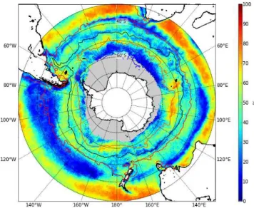
Fig. 1.Spatial distribution of mean chlorophyll concentrations for the Southern Ocean south of 30◦S for(a)summer–January and(b)winter–
July. Mean July and mean January (1998–2007) frontal positions calculated from MADT contours are shown for the STF (red), the SAF (black), the PF (orange) and the SACCF (blue).
at 40◦N to 23 % at 70◦N. During the summer months
how-ever, the zenith angle has little effect on the amount of sur-face reflectance which is generally between 4 and 7 % at all latitudes (40–70◦) and under all atmospheric and wind
con-ditions (Campbell and Aarup, 1989).
3 Results and discussion
3.1 Zonal characterization of seasonal biomass
variability
Remote sensing derived chlorophyll distributions in the Southern Ocean south of 30◦S reflect a zonal (annular)
char-acter of variability such as observed between frontal and pelagic zones as well as remarkable regional contrasts be-tween the Atlantic and Pacific Oceans (Fig. 1a). These spatial zones also display important seasonal contrasts (Fig. 1a, b). While technically an estimate of pigment concentrations, we use SeaWiFS surface chlorophyll as a proxy for phy-toplankton biomass (Sullivan et al., 1993; Comiso et al., 1993; Moore and Abbott, 2002). Satellite surface chloro-phyll concentrations do not however take into account deep chlorophyll maxima or changes in the carbon to chloro-phyll ratio (C:Chl-a) with depth. Although typical deep chlorophyll maxima in the subtropics may result in under-estimated satellite derived chlorophyll, chlorophyll profiles at higher latitudes (>40◦S) are typically uniform in the
upper mixed layer and decreases exponentially at greater depths (Arrigo et al., 2008). The lack of depth integrated chlorophyll distribution is thus unlikely to significantly effect satellite derived chlorophyll concentrations south of 40◦S.
Changes in C:Chl-a are associated with physiological re-sponses to changing light, temperature and nutrient
condi-tions and are lowest at high temperatures (25–30◦C), low
irradiances (<20 µmol photons m−2s−1and nutrient replete conditions and increase at high irradiances, low temperature and nutrient limiting conditions (Taylor et al., 1997). Al-though seasonal variability in C:Chl-aratios is significant at lower latitudes, the variations are relatively minor at higher latitudes when compared with the much larger seasonal range in chlorophyll concentration (Taylor et al., 1997). Although changes in C:Chl-a ratios need to be considered when us-ing satellite surface chlorophyll measurements as a proxy for biomass, existing data suggest that these intra-cellular C:Chl-aratios do not play a significant role in the seasonal cycle in the Southern Ocean (Taylor et al., 1997). In addition, stan-dard ocean colour algorithms typically underestimate chloro-phyll in the Southern Ocean by 2–3 times compared to in situ measurements (Kahru and Mitchell, 2010). Underes-timated chlorophyll concentrations are however unlikely to impact the characterisation of the patterns of the seasonal cy-cle which forms the primary focus of this paper.
In the subtropics, surface chlorophyll concentrations are low year round, except for a band of increased chlorophyll between 30◦and 40◦S in winter when nutrients are
replen-ished (Fig. 1b). Surface chlorophyll concentrations south of 40◦S are low during the austral winter when light levels are
around Antarctica. This band in the Pacific shows very little seasonal difference between summer and winter chlorophyll concentrations (Fig. 1a, b).
Lowest summer chlorophyll concentrations are associated with the pelagic waters north of the sea ice zone (Fig. 1a) where production rates are limited by deep mixing of the upper mixed layer and trace metal limitation (Mitchell and Holm-Hansen, 1991; Boyd et al., 2000; Sokolov and Rintoul, 2007a). An exception to these low production waters is found at oceanic frontal zones (Fig. 1a). Enhanced chlorophyll con-centrations associated with the major fronts of the ACC have been well documented and attributed to a number of pro-cesses that include cross-frontal mixing of macronutrients, an improved light environment through enhanced stratifica-tion and increased Fe concentrastratifica-tions through upwelling and interaction of the fronts with shallow topography (e.g. Lutjer-harms et al., 1985; Laubscher et al., 1993; Moore and Abbott, 2002). Although traditionally, enhanced chlorophyll concen-trations have been associated with mesoscale activities at the position of the fronts, Sokolov and Rintoul (2007b) more re-cently revealed that multiple frontal branches delimit regions with similar elevated chlorophyll concentrations and season-ality rather than the fronts themselves being associated with enhanced productivity, at least where fronts are distant from topography.
Another exception to low production Southern Ocean wa-ters is found over regions of shallow bathymetry; around and downstream of subantarctic islands, the continental shelf, over mid-ocean ridges and large plateaus (Fig. 1a). In these regions of shallow bathymetry, current flow through rela-tive vorticity (Hogg and Blundell, 2006; Moore et al., 1999) and/or bottom pressure torque (Sokolov and Rintoul, 2007a) is thought to increases the flux of Fe into surface waters (Park et al., 2010; Venables and Moore, 2010) accounting for the generally inverse correlation between depth and chloro-phyll in the Southern Ocean (Comiso et al., 1993). Highest chlorophyll concentrations are generally associated with the marginal ice zone (MIZ) (Fig. 1a) (Arrigo and van Dijken, 2004), through enhanced irradiance from increased vertical stratification when ice melts (Smith Jr. and Nelson, 1986), through Fe input from melting ice (Sedwick and DiTullio, 1997; Gao et al., 2003; Grotti et al., 2005) and mixing of Fe rich sediments along the continental shelf (Schoemann et al., 1998; Johnson et al., 1999). Atmospheric dust deposition downwind of dry continental areas (e.g. Patagonia, south and south west of Australia, New Zealand and Africa) is also con-sidered a dominant Fe source fertilising primary production in the Southern Ocean (e.g. Cassar et al., 2007).
3.2 The Seasonal cycle of chlorophyll in the Southern
Ocean
The characteristics of the seasonal cycle of phytoplank-ton biomass in the Southern Ocean are examined in terms of the timing of the bloom initiation, its amplitude,
inter-120°W 100°W 80°W
60°W 60°E
80°E
100°E
120°E
180° 160°W
140°W 160°E 140°E
40oS
60oS
Jan. Feb. Mar. Apr. May Jun. Jul. Aug. Sep. Oct. Nov. Dec.
date
Fig. 2. Date of the phytoplankton bloom initiation in the South-ern Ocean south of 30◦S. Mean (1998–2007) frontal positions
cal-culated from MADT contours shown for the STF (red), the SAF (black), the PF (orange) and the SACCF (blue).
annual variability (variability in the seasonal cycle from year to year) and intra-seasonal variability (variability of phyto-plankton biomass within a season) and the importance of the climatological seasonal cycle in explaining the overall vari-ance. The spatial distribution of the seasonal cycle is subse-quently defined to four zonal regions. The subtropical zone (STZ), the transition zone (TZ), the Antarctic circumpolar zone (ACZ) and the marginal ice zone (MIZ). The following section will describe the foundation for these zonal defini-tions based on seasonal characteristics rather than the dis-tribution of chlorophyll concentrations, which has generally been the case in previous Southern Ocean studies.
mixing is deepest. Behrenfeld’s dilution-recoupling hypoth-esis (Behrenfeld, 2010) challenges Sverdrup’s Critical Depth Hypothesis (Sverdrup, 1953) by de-emphasizing the role of light and instead suggesting a much greater role for the bal-ance between phytoplankton growth and losses through graz-ing. Although net population growth may increase in mid-winter, it is worth noting that chlorophyll concentrations and specific growth rates are at their seasonal minimum. Our definition of the chlorophyll bloom on the other hand coin-cides with peaks in phytoplankton productivity, CO2uptake and carbon export, all of which are products of phytoplank-ton biomass and specific growth rates (Boss and Behrenfeld, 2010). The annual cycles of phytoplankton biomass in our results emphasize the role of bottom-up controls (light and nutrients) on increases in phytoplankton specific growth rates for determining bloom initiation (Sverdrup, 1953). The lack of information on growth rates does not allow us to quantify the role of grazing. In this study, we do not assume that the role of grazing is negligible, but rather that statistically sig-nificant seasonal increases in biomass can only occur when specific growth rates exceed loss terms and net population growth remains positive, despite potential increases in graz-ing pressure associated with increased encounter rates when the seasonal mixed layer shallows.
According to Fig. 2, bloom initiation in the STZ (∼30– 40◦S), is characterized by an onset taking place in autumn
(April–June) when macro-nutrients are replenished with the deepening of the seasonal mixed layer. This STZ is well de-fined in its latitudinal extent. North of∼30◦S, insufficient
heat loss in winter limits the breakdown of stratification and deep winter overturning to below the nutricline preventing winter increases in chlorophyll biomass. South of∼40◦S, low winter PAR limits net primary productivity, preventing concomitant increases in winter chlorophyll concentrations, forcing phytoplankton populations towards spring bloom ini-tiations (September–November). With the exception of the central and eastern Pacific, the transition between autumn and spring bloom initiations is remarkably abrupt and indi-cates a rapid shift from one seasonal regime to another, rather than a monotonic progression in the timing of the bloom ini-tiation with increasing latitude. Further south is the MIZ where bloom initiation dates are in summer (December to February), reflecting the delay in seasonal PAR availability as well as the time it takes for phytoplankton blooms to fully respond to the newly created ice-free waters associated with the region (Arrigo et al., 2008). This was similarly shown to be the case in the Arctic where phytoplankton blooms took ∼20 days to respond to sea-ice melt (Perrete et al., 2011).
While the bloom onset in the STZ is spatially homoge-neous, waters south of 40◦S are characterized by large
spa-tial variability with bloom initiation dates that can occur as early as May (e.g. Crozet,∼45◦S, 50◦E) or as late as
Jan-uary (south of Tasmania,∼42◦S, 147◦E). The transition
be-tween zonally comparable regions of early and late bloom onset can be relatively abrupt: for example the region of early
120°W
100°W
80°W
60°W
60°E
80°E
100°E
120°E
180°
160°W
140°W
160°E
140°E
40oS
60oS
0 1 2 3 4 5 6 7 8 9 10 11 12 13 14 15
Standard Deviation (8-days composites)
Fig. 3. Inter-annual variability (standard deviation over the 9 yr) in phytoplankton bloom initiation dates (units in 8-day composites) for the Southern Ocean south of 30◦S.
(September, 100–140◦E) and late (December, 130–170◦E)
bloom development found south of Australia (50–55◦S) and
the region of early onset evident north east of Crozet where the spring bloom starts particularly early in the year (May).
Regions with high inter-annual variability (std. Dev. 10–16 units in 8-day composites) in bloom initiation dates (Fig. 3) generally correspond to regions of transition between differ-ent seasonal regimes. In particular the transition between autumn and spring bloom initiation centred around∼40◦S. The boundaries of this region of high variability in bloom initiation define what we term the TZ. Similar high variabil-ity in bloom initiation dates was found in the transition zone separating regions of winter bloom initiation in the subtrop-ical North Atlantic from May bloom initiations in the sub-polar North Atlantic (Henson et al., 2009). The remaining region of spring bloom initiation between the TZ and MIZ is what we term the ACZ. Other regions of high variabil-ity in bloom initiation similarly coincide with transition re-gions between different seasonal regimes, e.g. the region of late bloom initiation south of Australia (130–170◦E) and the
transition between spring and summer bloom initiation at the confluence of the ACZ and MIZ which is particularly ex-tended in the Atlantic and the western Indian Ocean sector (20◦W–60◦E). Although the shift in mean bloom initiation
Fig. 4. Percentage (from 0 to 1) of the overall variance explained by the mean seasonal cycle for the Southern Ocean south of 30◦S.
Masked grid-points in white correspond to areas where more than half of the weekly values are missing. Mean (1998–2007) frontal positions are shown for the STF (red), the SAF (black), the PF (green) and the SACCF (blue).
The percentage of the variance explained by the mean sea-sonal cycle (Fig. 4) defines how well the mean climatolog-ical seasonal cycle (from 9 yr) represents the evolution of chlorophyll over each year. Areas where the seasonal cycle for each year is coherent with the 9 yr mean (R2>0.4) are defined as having high seasonal cycle reproducibility. Re-gions where there is large variability from year to year in the timing and amplitude of the bloom, and only a low percent-age of the variance can be explained by the mean seasonal cycle (R2<0.4) are defined as having low seasonal cycle reproducibility. Immediately apparent from figure 4 is the sharp gradients between strongly contrasting regions of high (>70 %) and low (<30 %) seasonal cycle reproducibility.
Despite the weak amplitude of the seasonal cycle in the STZ (∼0 to 0.5 mg m−3)between summer minima and win-ter maxima, (Fig. 1a, b) (see also Allison et al., 2010) the overall variance of the chlorophyll signal is strongly phase locked to the mean seasonal cycle (>70 % of variance ex-plained) (Fig. 4). An example of the time series of chloro-phyll compared to the climatological mean seasonal in the STZ is shown in Fig. 5a. In this nutrient limited region, the phytoplankton seasonal cycle occurs in a predictable manner (R2=0.91, Fig. 5a) when seasonal net heat loss and over-turning in late autumn/early winter deepens the mixed layer to below the nutricline, relieving nutrient stress in surface waters and allowing phytoplankton production and biomass to increase. This finding agrees well with Dandonneau et al. (2004), who found low ratios of inter-annual to total vari-ance from monthly SeaWiFS chlorophyll concentrations in
the subtropical band between 1998 and 2001. Barton et al. (2010) developed a large-scale ocean model to investigate phytoplankton diversity across the global ocean and found that temporal variability of the environment played a signif-icant role on the ecological control of phytoplankton diver-sity. Regions with relatively steady environmental conditions and high seasonal cycle reproducibility, such as the subtrop-ics, enable the coexistence of multiple phytoplankton species and enhanced diversity (Barton et al., 2010).
In the ACZ and MIZ, the amplitude of the seasonal sig-nal is much higher (see also Allison et al., 2010) and large regions of relatively high seasonal cycle reproducibility are found, e.g. in the Pacific south of 50◦S (∼50 %), east of
Ker-guellen (∼49◦S, 70◦E) (60–80 %) and a finer scale banded
structure associated with the SAF zone and PF zone in the eastern Atlantic (50–70◦S, 0–10◦E) (Fig. 4). In
re-gions with a high degree of seasonal cycle reproducibility (e.g. Fig. 5b, c;R2=0.66 and 0.64, respectively) one would expect that intra-seasonal forcing does not play a significant role in the phytoplankton seasonal cycle and that the annual time series would be almost entirely explained by the sea-sonal forcing of light, heat flux and seasea-sonal MLD (as in the subtropics, e.g. Fig. 5a). This does not mean that Fe or light is not limiting but merely that it does not vary sufficiently on an intra-seasonal time scale to influence the inter-annual variability of the phytoplankton seasonal expression. In such instances one would expect there to be sufficient winter pre-conditioning of the water column with limiting nutrients (no-tably Fe) to allow a bloom initiation when the seasonal PAR threshold for increased primary production and biomass ac-cumulation is met in spring. The amplitude of the seasonal bloom would depend on the supply of Fe via mechanisms that include (a) the seasonal re-supply of Fe through winter overturning (wintertime convective mixing sets the available nutrients for new production; Dutkiewicz et al., 2001), (b) the depth of the summer mixed layer relative to the ferricline (deeper MLD’s having higher Fe reserves), (c) the amount of lateral advection of Fe into surface waters (e.g. downstream advection from continents and subantarctic islands), (d) the amount of Fe supplied by upwelling at fronts and (e) the de-livery of soluble iron by aerosol deposition (e.g. Fig. 5b and c for low [∼0.25 mg m−3] versus high [∼1 mg m−3] summer blooms, respectively). In these instances, the intra-seasonal re-supply of Fe to surface waters through wind mixing or mesoscale variability plays a less significant role in promot-ing phytoplankton growth, hence the low degree of intra-seasonal and inter-annual variability (Fig. 5b, c).
Regions of low seasonal cycle reproducibility (Fig. 4) gen-erally correspond to regions of high variability in the phasing of the bloom initiation (Fig. 3). The zone of low variance ex-plained by the mean seasonal cycle (<20 %) marks the TZ (∼40◦S). This region is particularly extensive in the Pacific
(∼40–50◦S), where chlorophyll concentrations are so low
1998 1999 2000 2001 2002 2003 2004 2005 2006 2007 0.05
0.10 0.15 0.20 0.25
Ch
lor
op
hy
ll-a
(m
g.m
−
3)
a) R2 = 0.91
1998 1999 2000 2001 2002 2003 2004 2005 2006 2007 0.10
0.15 0.20 0.25 0.30
Ch
lor
op
hy
ll-a
(m
g.m
−
3)
b) R2 = 0.66
1998 1999 2000 2001 2002 2003 2004 2005 2006 2007 0.2
0.4 0.6 0.8 1.0 1.2 1.4 1.6
Ch
lor
op
hy
ll-a
(m
g.m
−
3)
c) R2 = 0.64
1998 1999 2000 2001 2002 2003 2004 2005 2006 2007 0.08
0.10 0.12 0.14 0.16 0.18 0.20
Ch
lor
op
hy
ll-a
(m
g.m
−
3)
d) R2 = 0.27
1998 1999 2000 2001 2002 2003 2004 2005 2006 2007 0.5
1.0 1.5 2.0
Ch
lor
op
hy
ll-a
(m
g.m
−
3)
e) R2 = 0.44
Fig. 5.Time series of chlorophyll concentrations from 1998 to 2007 (in red) compared to the climatological mean seasonal cycle (calculated over the 9 yr) (in blue) for 5×5 degree blocks in(a)a region of high seasonal cycle reproducibility in the low chlorophyll STZ (30–35◦S,
0–5◦W),(b)a region of high seasonal cycle reproducibility in the low chlorophyll ACZ west of Kerguellen (50–55◦S, 55–60◦E),(c)a
region of high seasonal cycle reproducibility and high chlorophyll in the ACZ, downstream of Kerguellen (50–55◦S, 70–75◦E),(d)a region
of low seasonal cycle reproducibility and low chlorophyll in the TZ of the Pacific (40–45◦S, 95–100◦W) and(e)a region of low seasonal
cycle reproducibility and high chlorophyll in the TZ off the east coast of South America (40–45◦S, 50–55◦W). The percentage of variance
(e.g. Fig. 5d;R2=0.27). The transition between spring and summer bloom initiation at the ACZ and MIZ confluence also marks a region of low seasonal cycle reproducibility. At a smaller scale, transitions between regions of contrast-ing bloom initiation dates within the ACZ are also character-ized by weak seasonal cycle reproducibility e.g. the region of low variance explained by the seasonal cycle corresponding to the region of late bloom initiation south of Australia.
We hypothesize that low seasonal cycle reproducibility re-lated to the transition between regions of different bloom initiation is potentially related to the diversity of conditions encountered at the confluence between contrasting seasonal regimes. Transition regions of low seasonal cycle repro-ducibility are thought to be driven by a combination of mul-tiple limiting factors and forcing mechanisms from both sea-sonal regimes (e.g. nutrient and light limitation, see also Dutkiewicz et al., 2001 and Henson et al., 2009). If there are too many factors simultaneously limiting phytoplankton pro-duction (e.g. nutrients and light), phytoplankton are not able to optimise to their environment, restricting the ability of the system to build up biomass. The expression of this will mani-fest as low annual chlorophyll concentrations with high inter-annual and intra-seasonal variability in bloom characteristics such as are found at the TZ in the Pacific (Figs. 4, 5d).
Low seasonal cycle reproducibility (Fig. 4) does not how-ever necessarily coincide with low chlorophyll concentra-tions (Fig. 1a). The TZ of low seasonal cycle reproducibil-ity in the Atlantic and Indian has relatively high summer chlorophyll concentrations (e.g. Fig. 5e;R2=0.44; chloro-phyll max= ∼1 mg m−3). Likewise, low seasonal cycle re-producibility regions surrounding the continental margins of Antarctica, America and Africa (Fig. 4) reflect high summer chlorophyll concentrations (Fig. 1a). If our hypothesis for the low chlorophyll concentrations in the Pacific TZ holds true then there has to be a reduction in the number of factors simultaneously limiting production in regions of low sea-sonal cycle reproducibility but high chlorophyll. We propose that in these regions intra-seasonal physical forcing mech-anisms are sequentially relieving light and/or nutrients at a frequency that is long enough to allow phytoplankton blooms to fully develop. At the latitudes of the continental mar-gins of Africa and America for example, nutrients rather than light are considered the dominant limiting factor in summer. The upwelling of nutrients, particularly on eastern bound-aries, through periodic wind events relieves nutrient stress on a sub-seasonal time scale. The period of sub-seasonal forcing must optimise growth in biomass at rates that exceed losses to account for the high integrated summer chlorophyll concentrations found here (Pasquero et al., 2005). The sub-seasonal wind events responsible for the upwelling and mix-ing of nutrients are likely to be responsible for the high intra-seasonal and inter-annual variability expressed as low sea-sonal cycle reproducibility. Along the continental margins of Antarctica on the other hand, elevated Fe associated with the continental shelf and ice melt (Fitch and Moore, 2007)
makes light a potentially dominant limiting factor. Intra-seasonal forcing of the interaction between a deepening of the MLD through wind mixing and the re-establishment of stratification through fresh water buoyancy, at adequate time scales, similarly accounts for the high chlorophyll concen-trations but low seasonal cycle reproducibility found in this region. In regions such as these, where there is a low degree of seasonal cycle reproducibility, environmental variability (through changes in the MLD which regulates light and nu-trient availability) may lead to competitive exclusion and a reduction in phytoplankton diversity (Barton et al., 2010).
The supplementary discussion accompanying Figs. S1–S4 elaborates on intra-seasonal and inter-annual variability (that result in either high or low seasonal cycle reproducibility) and complements the zonal characterisation of the South-ern Ocean’s seasonal cycle. Inter-annual and intra-seasonal variability in the STZ is low and consistent with a high de-gree of seasonal cycle reproducibility (Fig. 4), whereas in the TZ, inter-annual and intra-seasonal variability is partic-ularly high and seasonal cycle reproducibility consequently weak. A well defined but short lived bloom is found in the ACZ, and although there is low variability in bloom initiation dates, inter-annual variability in the amplitude of the bloom is high. In the MIZ, variability in bloom initiation dates is low but both inter-annual and intra-seasonal variability in the chlorophyll seasonal cycle is high, leading to low seasonal cycle reproducibility.
Fig. 6.Average MLD in(a)winter (August) and(b)summer (February) in the Southern Ocean from the De Boyer Mont´egut et al. (2004) dataset.
is ultimately responsible for the observed variability in the chlorophyll seasonal cycle.
3.3 Mixed layer depth, irradiance and the
phytoplankton seasonal cycle
As expected, mean MLD’s for winter (August) are deeper than in summer (February) and present large spatial variabil-ity (Fig. 6a, b). In the Atlantic (∼20◦E–20◦W) and eastern
Indian Ocean (∼60–180◦E), MLD’s of >200 and >300 m
respectively are found between ∼40 and 50◦S in winter (Fig. 6a). Whereas in the Pacific in winter, (∼150–70◦W) MLD’s of>400 m are found further south between∼50 and 60◦S. In the 40–50◦S latitudinal band, MLD’s are relatively
shallow (∼80–140 m) in winter compared to similar latitudes in the Atlantic and Indian (Fig. 6a). In summer, MLD’s present a more zonally coherent distribution, with MLD’s shallower than∼50 m observed north of 40◦S and south of
60◦S, with MLD’s of 80–120 m in between (Fig. 6b).
The chlorophyll concentration at the sea surface gener-ally responds to the seasonal cycle of solar radiation which strongly impacts vertical stability through net heat flux, in-fluencing vertical nutrient supply and the timing and inten-sity of phytoplankton blooms (Dandonneau et al., 2004). A first order estimate of the large-scale relationship between the seasonal cycles of MLD and chlorophyll (Fig. 7) can there-fore be used to improve our understanding of the transition between different seasonal regimes.
Consistent with our understanding of the subtropics as a nutrient-limited regime, the correlation in the STZ is uni-formly positive (>0.8), with increased chlorophyll coincid-ing with deep winter MLD’s and associated nutrient replen-ishment. These findings are supported by a study in the sub-tropical North Atlantic where anomalously strong convective
120°W 100°W 80°W
60°W 60°E
80°E
100°E
120°E
180° 160°W
140°W 160°E 140°E
40oS
60oS
-1.0 -0.9 -0.8 -0.7 -0.6 -0.5 -0.4 -0.3 -0.2 -0.1 0.0 0.1 0.2 0.3 0.4 0.5 0.6 0.7 0.8 0.9 1.0
Pearson's R
Fig. 7.Pearson’s correlation coefficient between seasonal cycles of monthly MLD from the De Boyer Mont´egut et al. (2004) dataset and chlorophyll. Masked grid-points in grey correspond to ar-eas where more than half the monthly values were missing in the chlorophyll time series. Correlations are statistically significant at the 99 % confidence level.
mixing was shown to result in enhanced chlorophyll trations (Dutkiewicz et al., 2001). High chlorophyll concen-trations coinciding with deep MLD’s in the subtropics are likely enhanced by adjustments in community composition and photoadaptation of light limited cells in the deep winter mixed layer (Letelier et al., 1993).
reflecting the sharp climatological change in the response of the biology to the underlying physical control mechanisms. Negative correlations are evident in the ACZ and MIZ, con-sistent with a light limited regime where increased chloro-phyll concentrations coincide with shallow MLD’s (see also the subpolar regions of the North Altantic where deep mix-ing leads to lower phytoplankton abundances (Dutkiewicz et al., 2001). A shoaling of the MLD provides the required light environment for phytoplankton production favouring increases in specific growth rates that exceeds export and losses through grazing and results in biomass accumulation (Sverdrup, 1953; Mitchell et al., 1991; Comiso et al., 1993). However, in these high latitudes, low light (PAR) environ-ments, the relationship is more convoluted than in the sub-tropics, with areas of low and in some instances slightly posi-tive correlations (e.g. Crozet) interspersed among the general trend of a negative correlation. This “patchy” appearance is indicative of maximum seasonal chlorophyll concentrations that are not uniformly phased with the timing of minimum MLD’s. Unlike in the subtropics, where a simple overturning threshold (net heat loss in winter) initiates the seasonal cycle, the physical forcing mechanisms of the mixed layer dynam-ics south of 40◦S are more varied and complex, as are the
requirements to promote phytoplankton growth. Although the prevailing negative correlation between MLD and surface chlorophyll suggests that light is more important in limiting production in the subantarctic (relative to the subtropics), the Southern Ocean is also nutrient limited, in particular with regards to Fe and Si (Boyd et al., 2002). The prolonged per-sistence of a shallow mixed layer can in some cases lead to nutrient limitation of primary production such that a periodic intra-seasonal deepening of the mixed layer (allowing Fe re-supply), at time scales of the same order as the phytoplankton growth rate, is necessary to maintain production rates at high levels throughout the summer season (Pasquero et al., 2005). In such instances, phytoplankton population growth rates are able to exceed their losses resulting in a well defined seasonal phytoplankton bloom (the integrated effect of localised sub-seasonal blooms) that does not coincide with the shallowest MLD’s (see also Fauchereau et al., 2011).
Changes in the mixed layer result from the interaction of turbulent mixing, through wind stress, and buoyancy forcing, through air/sea heat fluxes, fresh water fluxes, entrainment and advection (geostrophic and Ekman). These two drivers (turbulent mixing and buoyancy forcing) compete to either strengthen stratification or destroy it. We propose that the complex nature of the controls on stratification and produc-tion in the Southern Ocean plays an instrumental role in the expression of seasonal, sub-seasonal and regional variability in chlorophyll concentrations and the seasonal cycle.
3.4 Basin scale meridional controls of the seasonal cycle
In addition to the broad zonality explored in the previous sec-tion, a large degree of zonal asymmetry exists in the
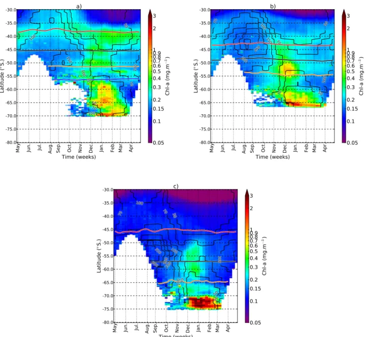
South-ern Ocean and provides the impetus for a comparison be-tween the main ocean basins. The zonally asymmetric nature of the seasonal cycle of chlorophyll in the Southern Ocean provides the impetus for basin scale comparisons in addi-tion to zonal characterisaaddi-tion. This asymmetry was similarly noted in the response of the MLD to the SAM by Sall´ee et al. (2010). From a heat budget of the mixed layer they con-clude that meridional winds associated with the departure of the SAM from zonal symmetry causes anomalies in heat flux and MLD which has consequences for biological productiv-ity. In the following section, particular emphasis is given to basin scale comparisons in order to more accurately charac-terise regional differences in the phasing of the chlorophyll bloom with respect to MLD’s. The seasonal progression of chlorophyll were plotted with mean MLD’s for three tran-sects, one in each of the ocean basins (Fig. 8a, b, c).
For each of the three transects a similar latitudinal pro-gression in seasonal characteristics of the chlorophyll bloom is evident (Fig. 8a, b, c). In the STZ to the north maximum chlorophyll concentrations are in winter, coincident with maximum winter MLD’s (50–130 m). Minimum chlorophyll concentrations occur in late summer, when MLD’s are shal-low (20–50 m). In the ACZ (south of the TZ), the phasing of the chlorophyll bloom switches to one in which maxi-mum concentrations are centred around the summer months (November to January), following the shoaling of the win-ter mixed layer (<70 m). In the MIZ bloom initiation oc-curs one month later (Fig. 2) with maximum concentrations extending into autumn (March) coinciding with shallowest MLD’s (30–40 m). The presence of the Weddell Gyre in the Atlantic transect (Fig. 8a) broadens the latitudinal extent of the MIZ (∼57–70◦S) compared to the Indian (∼60–65◦S) and Pacific (∼70–75◦S) (Fig. 8b, c).
Besides the comparable characteristics in latitudinal pro-gression of the seasonal cycle, inter-ocean basin differ-ences are also evident. The Atlantic and Indian transects (Fig. 8a, b) are characterised by a relatively rapid TZ (∼35– 40◦S). In the Pacific transect (Fig. 8c); the TZ between
win-ter and summer centred seasonal regimes is extended in lati-tude (35–49◦S), with distinct summer bloom characteristics
only evident south of 50◦S. The latitudinal transition to a
summer bloom regime coincides with the northernmost ex-pression of the deepest winter MLD’s i.e. 130 m in the At-lantic (42◦S), 300 m in the Indian (42◦S) and 300 m in the
Pacific (49◦S). Although the mechanism responsible for the
absence of a deep winter mixed layer in the 40–45◦S
lati-tudinal band in the Pacific (90–100 m) is unclear (see also Fig. 6a), it is likely that an additional sustained input of buoyancy (e.g. additional heat source from southward pen-etrations of subtropical water) prevents the deepening of the mixed layer in winter to depths comparable to those of the Atlantic and Indian (130 and 300 m, respectively).
May Jun. Jul. Aug. Sep. Oct. Nov. Dec. Jan. Feb. Mar. Apr.
Time (weeks)
-80.0 -75.0 -70.0 -65.0 -60.0 -55.0 -50.0 -45.0 -40.0 -35.0 -30.0
La
tit
ud
e (
o
S.)
a)
0.05
0.1
0.15
0.2
0.3
0.4
0.5
0.6
0.7
0.8
0.9
1
2
3
Ch
l-a
(m
g.m
−
3
)
May Jun. Jul. Aug. Sep. Oct. Nov. Dec. Jan. Feb. Mar. Apr.
Time (weeks)
-80.0 -75.0 -70.0 -65.0 -60.0 -55.0 -50.0 -45.0 -40.0 -35.0 -30.0
La
tit
ud
e (
o
S.)
b)
0.05
0.1
0.15
0.2
0.3
0.4
0.5
0.6
0.7
0.8
0.9
1
2
3
Ch
l-a
(m
g.m
−
3
)
May Jun. Jul. Aug. Sep. Oct. Nov. Dec. Jan. Feb. Mar. Apr.
Time (weeks)
-80.0 -75.0 -70.0 -65.0 -60.0 -55.0 -50.0 -45.0 -40.0 -35.0 -30.0
La
tit
ud
e (
o
S.)
c)
0.05
0.1
0.15
0.2
0.3
0.4
0.5
0.6
0.7
0.8
0.9
1
2
3
Ch
l-a
(m
g.m
−
3
)
Fig. 8.Mean seasonal cycles (May to April – x-axis) of chlorophyll (colour scale) and annual mean MLD in metres (contours) as a function of latitude (30–80◦S – y-axis) for a 10◦longitudinal transect in(a)the Atlantic (0–10◦E),(b)the Indian (85–95◦E) and(c)the Pacific
(110–100◦W) Oceans. Mean (1998–2007) frontal positions are shown for the STF (red), the SAF (black), the PF (orange) and the SACCF
(blue).
or subantarctic island and sub-ocean land mass and lower mesoscale eddy activity from a lack of bathymetry to inter-act with the mean flow. Increased eddy kinetic energy asso-ciated with such features, enhances the sub-surface flux of Fe into surface waters, potentially enhancing phytoplankton growth (Hense et al., 2000; Sokolov and Rintoul, 2007a; Park et al., 2010). If the main source of Fe to the surface waters of the Southern Ocean is through vertical mixing and upwelling 70–80 % (Archer and Johnson, 2000),>99 % (Lef`evre and Watson, 1999), one can deduce that in the Pacific, where Fe
supply to surface waters through deep water entrainment is limited, shallow winter mixed layers are unlikely to be deep enough to entrain sufficient Fe into the surface waters for stimulating and maintaining high production rates through the summer. This is consistent with a recent compilation of ∼13 000 dissolved iron measurements for the Southern Ocean (Tagliabue et al., 2011) which show comparatively low surface iron concentrations in the Pacific compared to the Indian and Atlantic. Hence, the extended (35–49◦S) low
seasonal cycle reproducibility, likely results from Fe limita-tion arising from a lack of adequate supply to the surface from the deep Fe pool.
4 Synthesis
Characterising the Southern Ocean according to the variabil-ity of the seasonal cycle provides a more dynamic under-standing of the spatial heterogeneity of production based on underlying physical drivers rather than mean climatological biomass. Based on our analysis of the timing, variability and seasonal cycle reproducibility of seasonal chlorophyll distributions, we defined the spatial distribution of the sea-sonal cycle into four zonal regions: (1) the STZ (∼30–35 or 40◦S), characterised by an autumn bloom initiation (Fig. 2),
low inter-annual and intra-seasonal variability and high sea-sonal cycle reproducibility (Fig. 4); (2) the TZ of high vari-ability in bloom initiation dates (centred around ∼40◦S) (Fig. 3), where inter-annual and intra-seasonal variability is also high and seasonal cycle reproducibility consequently weak (Fig. 4); (3) the ACZ (south of the TZ) where bloom initiations are generally in spring (Fig. 2), inter-annual vari-ability in bloom initiation dates is low (Fig. 3) and large ar-eas of both high and low sar-easonal cycle reproducibility are found (Fig. 4), and (4) the MIZ where bloom initiations are in summer (Fig. 2), variability in bloom initiation dates is low (Fig. 3) but inter-annual and intra-seasonal variability in the chlorophyll seasonal cycle is high, leading to low seasonal cycle reproducibility (Fig. 4).
This zonal classification effectively characterises the vari-ability of the seasonal cycle in the Southern Ocean. However, when the response of the biology to the underlying physics of the different seasonal regimes was taken into consideration (i.e. low versus high seasonal chlorophyll maxima), an addi-tional classification system was required. In order to sum-marise the varying responses of the phytoplankton commu-nity to the different seasonal regimes, we created a schematic that divides the Southern Ocean into a montage of four re-gions in addition to the four seasonal zones (Fig. 9). This schematic is created from a composite of the mean sum-mer chlorophyll concentration from November to February (1998–2007) and the variance explained by the seasonal cy-cle (Fig. 4). The four regions result from a combination of high (>0.25 mg m−3)or low (<0.25 mg m−3)chlorophyll concentration and high (R2>0.4) or low (R2<0.4) seasonal cycle reproducibility. This figure is intended as a support to a conceptual framework on the nature of the response of the phytoplankton seasonal cycle to variability in the physical control mechanisms.
Region A (light blue) is representative of a nutrient lim-ited regime with low chlorophyll concentrations but high sea-sonal cycle reproducibility. In Region A, in the STZ (30– 40◦S), nutrients (in particular NO
3)are limited throughout the summer months and it is only when the mixed layer
deepens in autumn that nutrient stress in surface waters is relieved, allowing phytoplankton production and biomass to increase. Similarly, Region A in the low chlorophyll pelagic waters of the Southern Ocean (north of the MIZ, away from fronts and shallow topographic features) is also nutrient lim-ited. Winter overturning re-supplies limiting surface nutri-ents (in particular Fe) to support an increase in phytoplank-ton growth, but only in spring when light levels are suffi-cient. In these regions, the available nutrients are rapidly used up by the phytoplankton community and the bloom sub-sequently declines when community losses outweigh growth rates. Despite the amplitude of the seasonal cycle in these regions being weak, the overall variability of the chlorophyll signal is strongly phase-locked to the annual seasonal cycle. In these regions, no sub-seasonal forcing of the mixed layer to below the nutricline is replenishing surface nutrients on seasonal time scales, which accounts for the low intra-seasonal and inter-annual variability and a predictable sea-sonal cycle (high seasea-sonal cycle reproducibility). According to ecological explanations for modelled diversity gradients, such stable environments are thought to favour multiple phy-toplankton with comparable fitness and subsequent high di-versity (Barton et al., 2010).
The second region with low chlorophyll concentrations (Region B, dark blue) is also characterised by low Fe con-centrations but this region displays low seasonal cycle repro-ducibility. This region is particularly extensive in the Pacific where increased positive buoyancy forcing potentially pre-vents the deepening of the winter mixed layer to below the ferricline, thus failing to re-set the seasonal Fe supply. If the winter re-supply of Fe to surface waters is insufficient and/or the depth of the ferricline is below the deepest summer MLD’s then phytoplankton lack the potential to significantly increase their biomass during the summer season through Fe limitation. These regions are characterised by chlorophyll concentrations that are so low and intra-seasonal variability so high that only a small percent of the variance (<20 %) can be explained by the mean seasonal cycle.
The last two regions refer to areas of high chlorophyll but with either a high (Region C, dark green) or low (Region D, light green) seasonal cycle reproducibility. Regions of high chlorophyll in the Southern Ocean result from integrated sea-sonal primary production that exceeds community losses and according to the literature results from the relief of Fe stress at ocean fronts, over shallow bathymetry, along continental margins, in the MIZ (e.g. Boyd, 2002) and downwind of dry continental areas (Cassar et al., 2007). The different seasonal expressions of high and low seasonal cycle reproducibility, however implies distinct physical supply mechanisms of Fe and light to the surface waters.
Fig. 9. A schematic summarising the response of phytoplankton biomass to the underlying physics of the different seasonal regimes. Regions in blue represent regions of low (<0.25 mg m−3)chlorophyll concentration with either high seasonal cycle reproducibility (R2> 0.4) (Region A, light blue) or low seasonal cycle reproducibility (R2<0.4) (Region B, dark blue). Regions in green represent regions of high chlorophyll concentration (>0.25 mg m−3)with either high seasonal cycle reproducibility (Region C, dark green) or low seasonal cycle reproducibility (Region D, light green). Mean (1998–2007) frontal positions are shown for the STF (red), the SAF (black), the PF (yellow) and the SACCF (pink).
is almost entirely explained by the seasonal forcing of light, heat flux and seasonal MLD (as in the subtropics). This is not to say that Fe or light are not limiting factors but merely that their influence does not vary sufficiently on intra-seasonal or inter-annual time scales to impact the high reproducibil-ity of the phytoplankton seasonal expression. In such in-stances sufficient winter preconditioning of the water column with limiting nutrients allows for a consistent bloom initia-tion when the seasonal PAR threshold is met in spring. The duration and integrated seasonal amplitude of the bloom de-pends on the amount of Fe made available through winter overturning, the depth of the summer mixed layer relative to the nutricline, lateral advection of Fe into surface waters, upwelling at fronts or dust deposition.
In regions of high chlorophyll but low seasonal cycle re-producibility (Region D, light green), the seasonal character-istics of high inter-annual and intra-seasonal variability are likely to be controlled by sub-seasonal forcing of the nutri-ent and light supply. In these regions, we hypothesize that high integrated summer chlorophyll concentrations are a di-rect consequence of high intra-seasonal physical forcing of the MLD at appropriate time scales (Pasquero et al., 2005). In these regions, shallow MLD’s likely lead to short term
de-pletions of surface nutrients such that a periodic deepening of the ML (to below the nutricline) is necessary for phytoplank-ton population growth to occur. This high intra-seasonal vari-ability likely culminates from a combination of high wind stress variability at appropriate time scales and upper water column stabilisation through positive buoyancy forcing via mesoscale dynamics and fresh water (ice melt) fluxes. In regions such as these, where the seasonal variability of the environment is high, competitive exclusion of phytoplankton with slower growth rates may lead to lower phytoplankton diversity (Barton et al., 2010).
the trajectory of primary production through the food web, influencing the proportion of biomass exported to the deep sea (Finkel et al., 2010). Looking to the future, the devel-opment of ecosystem appropriate functional type algorithms will allow us to use satellite remote sensing data to provide information on the response of phytoplankton community composition and physiology to physically distinct seasonal regimes and ultimately to climate change.
Although the fronts of the STF and ACC clearly influ-ence the regional characterisation of the seasonal cycle of chlorophyll in the Southern Ocean (Fig. 9), the physical forc-ing mechanisms responsible for enhanced chlorophyll (large scale flow versus small scale instabilities) are still unclear and need to be investigated further.
The seasonal cycle is the mode that couples the physi-cal mechanisms of climate forcing to ecosystem response in production, diversity and carbon export. Accordingly, long term trends in Southern Ocean productivity will be mediated through changes in the characteristics of the seasonal cycle and its interaction with the phenology of the ecosystem. Our regionalisation of the Southern Oceans seasonal cycle may therefore be important in assessing potential regional dif-ferences in the response of the biological pump to climate change. Future studies that better address the mechanisms governing this spatial variability will allow us to make more robust predictions of the Southern Oceans carbon cycle.
Appendix A
Acronyms.
Southern Annular Mode SAM
Subtropical Zone STZ
High Nitrate Low Chlorophyll HNLC
Iron Fe
Sea-viewing Wide Field of view Sensor SeaWiFS Maps of Absolute Dynamic Topography MADT Antarctic Circumpolar Current ACC
Subantarctic Front SAF
Polar Front PF
Southern Antarctic Circumpolar SACCF Current Front
Subtropical Front STF
Mixed Layer Depth MLD
Photosynthetically Active Radiation PAR
Subtropical Zone STZ
Transition Zone TZ
Antarctic Circumpolar Zone ACZ
Marginal Ice Zone MIZ
Supplementary material related to this article is available online at:
http://www.biogeosciences.net/8/2849/2011/
bg-8-2849-2011-supplement.pdf.
Acknowledgements. This work was undertaken and supported through the Southern Ocean Carbon and Climate Observatory
(SOCCO) Programme. In addition, this work was partially
funded by the European Commission 7th framework program through the GreenSeas Collaborative Project, FP7-ENV-2010 contract No. 265294. S. J. Thomalla and S. Swart were supported through SOCCO post doctoral fellowships funded by ACCESS and NRF/SANAP SNA2007051100001. P. M. S. Monteiro and N. Fauchereau were supported by CSIR’s Parliamentary Grant. We would like to thank our anonymous reviewers for their valuable contribution to the improvement of this manuscript.
Edited by: E. Boss
References
Allison, D. B., Stramski, D., and Mitchell, B. G.: Seasonal and interannual variability of particulate organic carbon within the Southern Ocean from satellite ocean colour observations, J. Geo-phys. Res., 115, C06002, doi:10.1029/2009JC005347, 2010. Archer, D. E. and Johnson, K.: A model of the iron cycle in the
ocean, Global Biogeochem. Cy., 14, 269–279, 2000.
Arrigo, K. R. and van Dijken, G. L.: Annual changes in sea-ice, chlorophyll a, and primary production in the Ross Sea, Antarc-tica, Deep-Sea Res. Pt. II, 51, 117–138, 2004.
Arrigo, K. R., van Dijken, G. L., and Bushinsky, S.: Primary pro-duction in the Southern Ocean, 1997–2006, J. Geophys. Res., 113, C08004, doi:10.1029/2007JC004551, 2008.
Barton, A. D., Dutkiewicz, S., Flierl, G., Bragg, J., and Follows, M.: Patterns of diversity in marine phytoplankton, Science, 327, 1509, doi:10.1126/science.1184961, 2010.
Behrenfeld, M. J.: Abandoning Sverdrup’s critical depth hypothe-sis, Ecology, 91, 977–989, doi:10.1890/09-1207.1, 2010. Blain, S., Queguiner, B., Armand, L., Belviso, S., Bombled, B.,
Bopp, L., Bowie, A., Brunet, C., Brussaard, C., Carlotti, F., Christaki, U., Corbiere, A., Durand, I., Ebersbach, F., Fuda, J., Garcia, N., Gerringa, L., Griffiths, B., Guigue, C., Guillerm, C., Jacquet, S., Jeandel, C., Laan, P., Lefevre, D., Lo Monaco, C., Malits, A., Mosseri, J., Obernosterer, I., Park, Y., Picheral, M., Pondaven, P., Remenyi, T., Sandroni, V., Sarthou, G., Savoye, N., Scouarnec, L., Souhaut, M., Thuiller, D., Timmermans, K., Trull, T., Uitz, J., van Beek, P., Veldhuis, M., Vincent, D., Viollier, E., Vong, L., and Wagener, T.: Effect of natural iron fertilization on carbon sequestration in the Southern Ocean, Nature, 446, 1070– 1074, 2007.
B¨oning, C. W., Dispert, A., Visbeck, M., Rintoul, S. R., and Schwarzkopf, F.: The response of the Antarctic Circumpolar Current to recent climate change, Nat. Geosci., 1, 864–869, 2008.
Boss, E. and Behrenfeld, M.: In situ evaluation of the initiation of the North Atlantic phytoplankton bloom, Geophys. Res. Lett., 37, L18603, doi:10.1029/2010GL044174, 2010.
Boyd, P. W.: Environmental factors controlling phytoplankton pro-cesses in the Southern Ocean, J. Phycol., 38, 844–861, 2002. Boyd, P. W., Watson, A., Law, C. S., Abraham, E., Trull, T.,
Mur-doch, R., Bakker, D. C. E., Bowie, A. R., Charette, M., Croot, P., Downing, K., Frew, R., Gall, M., Hadfield, M., Hall, J., Harvey, M., Jameson, G., La Roche, J., Liddicoat, M., Ling, R., Maldon-ado, M., McKay, R. M., Nodder, S., Pickmere, S., Pridmore, R., Rintoul, S., Safi, K., Sutton, P., Strzepek, R., Tanneberger, K., Turner, S., Waite, A., and Zeldis, J.: A mesoscale phytoplankton bloom in the polar Southern Ocean stimulated by iron fertiliza-tion, Nature, 407, 695–702, 2000.
Boyd, P. W., Crossley, A. C., DiTullio, G. R., Griffiths, F. B., Hutchins, D. A., Queguiner, B., Sedwick, P. N., and Trull, T. W.: Effects of iron supply and irradiance on phytoplankton processes in subantarctic waters south of Australia, J. Geophys. Res., 106, 573–584, 2001.
Cassar, N., Bender, M. L., Barnett, B. A., Songmiao, F., Moxim, W. J., Levy II, H., and Tilbrook, B.: The Southern Ocean biological response to Aeolian iron deposition, Science, 317, 1067–1070, 2007.
Caldeira, K. and Duffy, P. B.: The role of the Southern Ocean in uptake and storage of anthropogenic carbon dioxide, Science, 87, 620–622, doi:10.1126/Science.287.5453.620, 2000.
Campbell, J. W.: The lognormal distribution as a model for bio-optical variability in the sea, J. Geophys. Res., 100, 13237– 13254, 1995.
Campbell, J. W. and Aarup, T.: Photosynthetically available radia-tion at high latitudes, Limnol. Oceanogr., 34, 1490–1499, 1989. Comiso, J. C., McClain, C. R., Sullivan, C. W., Ryan, J. P., and
Leonard, C. L.: Coastal Zone Color Scanner pigment concen-trations in the Southern Ocean and relationships to geophysical surface features, J. Geophys. Res., 98, 2419–2451, 1993. Davidson, I. R.: Environmental effects on algal photosynthesis:
Temperature, J. Phycol., 27, 2–8, 1991.
De Baar, H. J. W., De Jong, J. T. M., Bakker, D. C. E., Loscher, B. M., Veth, C., Bathmann, U., and Smetacek, V.: Importance of iron for plankton blooms and carbon dioxide draw-down in the Southern Ocean, Nature, 373, 412–415, 1995.
De Boyer Mont´egut, C., Madec, G., Fischer, A. S., Lazar, A., and Iudicone, D.: Mixed layer depth over the global ocean: An ex-amination of profile data and a profile-based climatology, J. Geo-phys. Res., 109, C12003, doi:10.1029/2004JC002378, 2004. Dandonneau, Y., Deschamps, P. Y., Nicolas, J. M., Loisel, H.,
Blan-chot, J., Montel, Y., Thieuleux, F., and Becu, G.: Seasonal and interannual variability of ocean color and composition of phy-toplankton communities in the North Atlantic, equatorial Pacific and South Pacific, Deep-Sea Res. Pt. II, 51, 303–318, 2004. Dutkiewicz, S., Follows, M., Marshall, J., and Gregg, W. W.:
In-terannual variability of phytoplankton abundances in the North Atlantic, Deep-Sea Res. Pt. II, 48, 2323–2344, 2001.
Fauchereau, N., Tagliabue, A., Monteiro, P., and Bopp, L.: The response of phytoplankton biomass to transient mixiing events in the Southern Ocean, Geophys. Res. Lett., 38, L17601, doi:10.1029/2011GL04849, 2011.
Finkel, Z. V., Beardall, J., Flynn, K. J., Quigg, A., Rees, T. A. V., and Raven, J. A.: Phytoplankton in a changing world: cell
size and elemental stoichiometry, J. Plankton Res., 32, 119–137, 2010.
Fitch, D. T. and Moore, J. K.: Wind speed influence on phytoplank-ton bloom dynamics in the Southern Ocean Marginal Ice Zone, J. Geophys. Res., 112, C08006, doi:10.1029/2006JC004061, 2007. Follows, M. and Dutkiewicz, S.: Meteorological modulation of the North Atlantic spring bloom, Deep-Sea Res. Pt. II, 49, 321–344, 2002.
Gao, Y., Fan, S., and Sarmiento, J. L.: Aeolian iron input to the ocean through precipitation scavenging: A modeling perspective and its implication for natural iron fertilization in the ocean, J. Geophys. Res., 108, 4221, doi:10.1029/2002JD002420, 2003. Gille, S. T.: Decadal-scale temperature trends in the Southern
Hemisphere ocean, J. Climate, 21, 4749–4765, 2008.
Glover, D. M., Doneym, S. C., Nelsonm, N. B., and Wallis, A.: Sub-mesoscale anisotropy (fronts, eddies, and filaments) as observed near Bermuda with ocean color data, Presented at Ocean Science Meet., Orlando, 2008.
Grotti, M., Francesco, S., Carmela, I., and Roberto, F.: Trace met-als distributions in coastal sea ice of Terra Nova Bay, Ross Sea, Antarctica, Antarct. Sci., 17, 290–300, 2005.
Hense, I., Bathmann, U. V., and Timmermann, R.: Plankton dynam-ics in frontal systems of the Southern Ocean, J. Marine Syst., 27, 235–252, doi:10.1016/S0924-7963(00)00070-1, 2000.
Henson, S. A. and Thomas, A. C.: Interannual variability in timing of bloom initiation in the California Current System, J. Geophys. Res., 112, C08007, doi:10.1029/2006JC003960, 2007.
Henson, S. A., Dunne, J. P., and Sarmiento, J. L.: Decadal variabil-ity in North Atlantic phytoplankton blooms, J. Phys. Oceanogr., 114, C04013, doi:10.1029/2008JC005139, 2009.
Hogg, A. M. and Blundell, J. R.: Interdecadal variability of the Southern Ocean, J. Phys. Oceanogr., 36, 1626–1645, 2006. Johnson, K. S., Chavez, F. P., and Friederich, G. E.:
Continental-shelf sediment as a primary source of iron for coastal phytoplank-ton, Nature, 398, 697–700, 1999.
Kahru, M. and Mitchell, B. G.: Blending of ocean colour algorithms applied to the Southern Ocean, Remote Sensing Letters, 1, 119– 124, 2010.
Kahru, M., Mitchell, B. G., Gille, S. T., Hewes, C. D., and Holm-Hansen, O.: Eddies enhance biological production in the Weddell-Scotia Confluence of the Southern Ocean, Geophys. Res. Lett., 34, L14603, doi:10.1029/2007GL030430, 2007. Kahru, M., Brota, V., Manzano-Sarabia, M., and Mitchell, B. G.:
Are phytoplankton blooms occurring earlier in the Arctic? Glob. Change Biol., doi:10.1111/j.1365-2486.2010.02312.x, in press, 2011.
Laubscher, R. K., Perisinotto, R., and Mcquaid, C. D.: Phytoplank-ton production and biomass at frontal zones in the Atlantic sector of the Southern Ocean, Polar Biol., 13, 471–481, 1993. Lef`evre, N. and Watson, A. J.: Modeling the geochemical cycle of
iron in the oceans and its impact on atmospheric CO2 concentra-tions, Global Biogeochem. Cy., 13, 727–736, 1999.