46
Simulation of Equal Poloidal Magnetic Flux Surfaces by Surfer
Software in Tokomaks
Shervin Saadat1*, Azadeh Haghighatzadeh1, Simin Nazari2
1
Department of Physics, Ahvaz Branch, Islamic Azad University, Ahvaz, Iran
2
Department of chemistry, Susangerd Branch, Islamic Azad University, Susangerd, Iran
*Corresponding author: shervin.saadat@gmail.com
Abstract
The tomography has played a key role in tokamak researches, and various tomographic methods were developed and used in the last several decades. The plasma cross sections were obtained by using laser arrays, but in this manuscript we used from mirnov coils. Our analysis is based on numerical method and mirnov coils data by surfer software to estimate equal poloidal magnetic flux surfaces in tokomaks.
Keywords: Tokamak, Equal poloidal magnetic flux surfaces, Plasma simulation, natural network, surfer software.
I. Introduction
Tomography has played a key role in tokamaks, and various tomographic methods were developed and used in the last several decades. Three methods for high special resolution (Arhatari et al.,2006).
• minimum Fisher information(MFI) • fast maximum entropy method (MEM) • Phillips-Tikhonov method (PTM)
Tomographic inversion can be obtained by various methods. The reconstruction method employed in most experiments is based on the analysis reconstruction algorithm, including the Cormack technique and Bessel expansion. Cormack uses expansion polynomials like these:
f , ( p) = ∑∞ a sin[(m + 2l + 1) cos p] (1)
g , ( p) = ∑∞ ( m + 2 l + 1) a
R ( r) (2)
Where,
R ( r) = ∑ ( ) ( )!
!( ) !( )! ∞
(3)
are called the Zernicke polynomials (Wang et al., 1991). The Bessel expansion was used like this,
g (r ) = J ( r) (4)
47
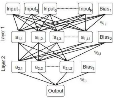
A Neural Network (NN) consists of simple processing units (neurons) connected amongst each other in a particular way. Typically, a NN is arranged in layers of neurons, where anyone neuron can have a connection to all other neurons on the previous layer.
Figure 1. A multilayer perceptron Neural Network, with 2 hidden layers. Each neuron is a function of all neurons on the previous layer and the bias. The bias neuron is independent of previous layers.
Each neuron has one activation function which can be any function of neurons from the previous layer(s). The activation function z used in this work is z = tan h(∑ w a )where a is the output from the neuron i of the previous layer and wi is the weight that neuron i has on the present neuron.
There are many types of NNs. In this work, a multi-layer perceptron was used. A NN must be trained in order to determine the weights. This training is done with an artificial input and output data set. For tomography, one generates a set of phantoms of expected spacial radiation distributions of the plasma and, using virtual sensors on this phantom, generates the corresponding sensor data. For this work, the phantoms generated were rings of different widths, radii and positions, because it makes sense that the H radiation is coming from the outer part of the plasma.
48
The considered methods are the Fourier-Bessel (Toussaint et al., 2006), and a neural-network (NN) method (Wang et al., 1991). In the fusion community, several tomography algorithms are used, the most common being the constrained regularization, also called pixel-based methods, Cormack based methods and Neural-Networks. The most common constrained regularization methods are the high Entropy and the Minimum Fisher, but other simpler regularizations exist. Expansion on the poloidal plane and an expansion in Zernicke polynomials in the radial direction. However, Zernicke polynomials have the inherent problem that they are non zero at the outer edge which can lead to completely unrealistic results. So a different type of functions must be used in the radial expansion and Wang (Wang et al., 1991) found that the first order Bessel functions are proper.
II. Spatial Interpolation Techniques
Interpolation refers to the process of estimating the unknown data values for specific locations using the known data values for other points. In many instances we may wish to model a feature as a continuous field like, 'surface', but we only have data values of points. It therefore becomes necessary to interpolate the values for the intervening points.
Interpolation methods may also be classified as exact or inexact. Using exact interpolation, the predicted values at the points for which the data values are known will be the known values; inexact interpolation methods remove this constraint (i.e. the observed data values and the interpolated values for a given point are not necessarily the same). Inexact interpolation may produce a smoother (and arguably more plausible) surface. Interpolation methods may be either deterministic or stochastic. Deterministic methods provide no indication of the extent of possible errors, whereas stochastic methods provide probabilistic estimates. Interpolation involves making estimates of the value of a quality variable at points for which we have no information using the data for a sample of points where we do have information. In general the more sample points we have the better. Likewise it is best to have a good spread of sample points across the study area. The general procedure is to identify a lattice of points for which data values are to be estimated. For each point, the procedure involves the following steps:
1. A search area (neighborhood) is defined around the point; 2. The sample points within the search area are identified;
3. A mathematical function is selected to model the local variation between these points: 4. The data value for the point is estimated from the function.
Different results will tend to arise depending upon the size of the search area and the type of mathematical function selected.
The value of a random variable Z at x is given as:
Z(x) = m( x) + ε,(x) + ε,,
where m( x) is a structural function describing the structural component,ε,(x) is the stochastic but spatially autocorrelated residuals from m( x) (i.e. the regionalized variable), and ε,, is random noise having a normal distribution with a mean of 0 and a variance σ .
49
E[Z( x)−Z( x + h) ] = 0
It is also assumed that the variance of the differences is a function of the distance between the points (i.e. they are spatially auto correlated, meaning that near points are more likely to have similar values, or smaller differences, than distant points) - i.e.
E[{Z( x)−Z(x + h) } ] = E[{ε,( x)− ε,(x + h) } ] = 2γ( h)
Where γ( h) is known as the semivariance. Under these two assumptions (i.e. stationarity of difference and stationarity in the variance of differences), the original model can be expressed as:
Z( x) = m( x) + γ(h) + ε,,
The semi variance can be estimated from the sample data using the formula:
γ ( h) =
{ ( ) ( )}
where n is the number of pairs of sample points separated by distanceh.
The semi variance can be calculated for different values of h. A plot of the calculated semivariance values against h is referred to as an experimental variogram.
III. Experimental details
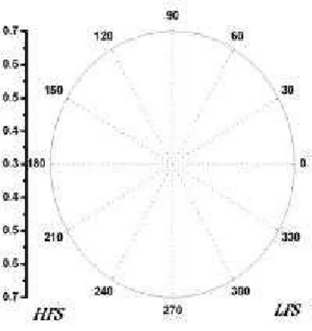
In this study, we used the data for mirnov coils IR-T1, a small tokamak with air core. The coils are located 120mm from the vacuum vessel center. The poloidal array formed by coils 1-12 (Figure2).
Figure 2. Mirnov coils geometry in IR-T1 tokamak.
50
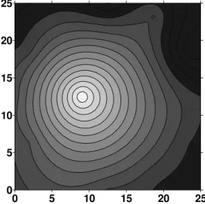
Although the investigator can choose between different types of kriging, kriging is less susceptible to arbitrary decisions taken by the investigator (e.g. search distance, number of sample points to use, location of break points, etc.). Kriging identifies the optimal interpolation weights and search radius. We use mirnov coils data and geometry of IR-T1 tokomak with local interpolation technique by surfer software and we determine equal poloidal magnetic flux surfaces at 17.5 ms shows in figure (3).
Figure 3. Equal poloidal magnetic flux surfaces at 17.5 ms.
The result shows Equal poloidal magnetic flux surfaces. The center of poloidal magnetic flux surfaces shifts to the left. The cross section of plasma shows plasma mode No. 3 and we can see the disruption and magnetic island in top of figure. Equal poloidal magnetic flux surfaces show clearly Grad-Shafranov (Bagerpour et al., 2015) shift and correct No. of plasma mode from the other techniques i.e. FFT, SVD and X-rays(Saadat et al., 2010,2011).The plasma cross sections obtained by using laser arrays, but in this method we use from mirnov coils.
IV. Results and discussion
One of the most practical problems of plasma tomography is the laser arrays instruments. This is a serious limitation for small tokamaks. In this work we have proposed a new method for determine equal poloidal magnetic flux surfaces of a small tokamak plasma using mirnov coils arrays. Our analysis is based on numerical method named kriging by surfer software. Surfer’s sophisticated interpolation engine transforms your XYZ data into publication-quality maps. Surfer provides more gridding methods and more control over gridding parameters, including customized variograms, than any other software package on the market. You can also use grid files obtained from other sources, such as USGS DEM files or ESRI grid files. Display your grid as outstanding contour, 3D surface, 3D wireframe, watershed, vector, image, shaded relief, and viewshed maps. Add base maps to show boundaries and imagery, post maps to show point locations, and combine map types to create the most informative display possible. Virtually all aspects of your maps can be customized to produce exactly the presentation you want. Generating publication quality maps has never been quicker or easier. Our 12 mirnov coils are modeled by a Gaussian process governed by prior covariance, as opposed to a piecewise-polynomial spline chosen to optimize smoothness of the fitted this values. The poloidal magnetic flux surfaces at 17.5 ms determined by this new method (Figure3).
0 5 10 15 20 25
51
V. Conclusions
The plasma cross sections obtained by using laser arrays, but in this method we use from mirnov coils that it is most useful for detect plasma cross section when there is not laser arrays. This simple method has been used extensively. This method uses the data of the mirnov coils arrays. The main difference here is those laser arrays used to measure the plasma magnetic flux surfaces, are complex and expensive instruments for small tokamaks and bigger, but the mirnov coils are accessible and applicable for all tokamaks. This method is most useful for the detect cross section and plasma mode number (Raju et al., 2000) .
References
i. Arhatari B D, Peele A G, Nugent K A and De Carlo F 2006 Quality of the reconstruction in x-ray phase contrast tomography Rev. Sci. Instrum. 77, 063709.
ii. Bagerpour M, AlinejadN and Sobhanian S 2015 Preliminary conceptual design of a medium sized tokamak Indian J. of Phys. 89 869.
iii. Raju D, Jha R, Kaw P K and Sexena Y C 2000 Mirnov coil data analysis for tokamak ADITYA
Pramana J. of Phys. 55 727.
iv. Saadat Sh, Salem M K, Ghoranneviss M and Khorshid P 2010 Mode analysis with autocorrelation method (single time series) in tokamak J. Fusion Energy 29 371.
v. Saadat Sh and Salem M K 2011 Comparison autocorrelation method and SVD method for plasma mode analysis in tokamaks J. Fusion Energy 30 342.
vi. Toussaint U V, Gori S and Dose V 2006 Invariance priors for Bayesian feed-forward neural network
Neural Networks 19 1550.