Revista Brasileira de Ensino de F´ısica,v. 30, n. 4, 4304 (2008) www.sbfisica.org.br
Strongly coupled overdamped pendulums
(Pˆendulos superamortecidos fortemente acoplados)R. De Luca
1Dipartimento di Matematica e Informatica, Universit`a degli Studi di Salerno, Fisciano, SA, Italy
Recebido em 12/5/2008; Aceito em 4/7/2008; Publicado em 27/2/2009
It is shown, by a first-order perturbation expansion, that the dimensionality of the dynamical equations for the angular variables of two strongly coupled identical overdamped pendulums can be reduced from two to one. The resulting dynamical equation is seen to be similar to the one of a single pendulum with an additional fictitious torque characterized by a second harmonic contribution.
Keywords: non-linear ordinary differential equations, coupled pendulums.
Mostra-se atrav´es de uma expans˜ao de perturba¸c˜ao de primeira ordem que a dimensionalidade das equa¸c˜oes dinˆamicas das vari´aveis angulares de dois idˆenticos e fortemente acoplados pˆendulos superamortecidos podem ser reduzida para apenas uma. A equa¸c˜ao dinˆamica resultante ´e similar `aquela de um pˆendulo simples com um torque fict´ıcio adicional caracterizado por uma contribui¸c˜ao de segundo harmˆonico.
Palavras-chave: equa¸c˜oes diferenciais n˜ao-lineares; pˆendulos acoplados.
1. Introduction
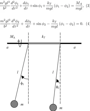
The angular variables φ1 and φ2 of two equal pendu-lums are shown in Fig. 1. The dynamics of this system is described by two coupled second-order non-linear dif-ferential equations in φ1 and φ2. The order of these equations can be reduced to one in the case of over-damped pendulums having small masses and moving in a viscous environment. Therefore, overdamped iden-tical strongly coupled pendulums can be described by a single differential equation for the average angular po-sitionφ= φ1+2φ2 of the two pendulums with respect to a common reference axis.
Indeed, one can solve for the difference between the two angular positionsψ= φ1−φ2
2 in terms ofφby means of a first order perturbation analysis, so that, upon sub-stitution of this solution in the time evolution equation forφ, one can obtain an effective one-dimensional model for the whole system. Analytic solution of this system provides an approximated solution to the system dy-namics.
The paper is organized as follows. In the next section, the equations for the two coupled pendulums are briefly derived and the perturbation solutions are found. In the third section the effective potential en-ergy for the system is found in terms of the average angular position φ and the time average of the angu-lar frequency is found in terms of a constant externally
applied torque. Finally, in the last section, conclusions are drawn and a brief discussion on the analogy of this system with a symmetric d. c. SQUID [1] is made.
2.
Dynamical equations and
perturba-tive expansion
Consider the mechanical system shown in Fig. 1, con-sisting of two identical pendulums of massmand length
l, coupled by a massless rod with torsional spring con-stantkT and freely rotating about the axisa−a. If a
torqueMA is applied on the system, the angular
devi-ations of the pendulums from their vertical equilibrium positions are indicated asφ1 andφ2, respectively. The mechanical system is immersed in a fluid with damp-ing constantb, so that the dynamical equations for the angular variablesφ1 andφ2 can be written as follows
MA−bdφ1
dt −mglsinφ1−kT(φ1−φ2) =ml 2d2φ1
dt2 , (1)
−bdφ2
dt −mglsinφ2+kT(φ1−φ2) =ml 2d2φ2
dt2 , (2) where we have assumed that the rigid rods, connect-ing the point mass of the pendulums and the rotatconnect-ing shaft, are massless. We now introduce the normalized
1E-mail: [email protected].
4304-2 De Luca
time τ = mglb t, so the system of equations (1a-b) be-comes
m2gl3 b2
d2φ1 dτ2 +
dφ1
dτ +sinφ1+ kT
mgl(φ1−φ2) = MA mgl, (3)
m2gl3 b2
d2φ 2 dτ2 +
dφ2
dτ + sinφ2− kT
mgl(φ1−φ2) = 0. (4)
f1
f2
m l
m l kT M
A
a a
Figure 1 - Two identical pendulums of massmand length
l, coupled by a massless rod with torsional spring constant
kT and freely rotating about the axisa−a. A torque MA
is applied on the system. The angular deviations of the pendulums from their vertical equilibrium positions are in-dicated asφ1 andφ2, respectively. The mechanical system
is immersed in a fluid with damping constantb.
In the overdamped case, we may set m2bgl23 <<1, so
that the above set of equations simplify to the following
dφ1
dτ + sinφ1+ kT
mgl(φ1−φ2) = MA
mgl, (5)
dφ2
dτ + sinφ2− kT
mgl(φ1−φ2) = 0. (6)
Let us now introduce the adimensional parame-ters β = mglk
T and mA = MA
kT , and the new variables φ= φ1+2φ2 and ψ= φ1−φ2
2 . By algebraic manipulation we can thus rewrite Eqs. (3a-b) in the following final form
dφ
dτ + sinφcosψ= mA
2β , (7)
dψ
dτ + cosφsinψ+
2ψ
β =
mA
2β . (8)
The above set of equations is not just rewritten in a different form, where the coupling has now represented by trigonometric functions rather than by linear func-tions as in Eqs. (3a-b). For small values of β, indeed,
we can try to solve Eq. (8) by means of a first-order perturbation analysis with respect to the same parame-terβ [2]. Assumingβ small, we thus set
ψ(τ) =mA
4 +βψ1(τ) +O
¡ β2¢
. (9)
Substituting Eq. (9) into Eq. (8), we obtain
ψ1(τ) =− 1
2cosφsin
³mA
4
´
. (10)
By having now solved forψ(τ) in terms of φ(τ) to first order in the parameterβ, we substitute the expres-sionψ(τ) =mA
4 − β 2sin
¡mA
4
¢
cosφinto Eq. (7) to get, consistently with the first order approximation in β
dφ dτ + cos
³mA
4
´
sinφ+β 4 sin
2¡mA 4
¢
sin 2φ=
mA
2β . (11)
The above equation, together with Eqs. (4) and (9), represents a reduced model for the prob-lem of two coupled overdamped identical pendulums. We notice that the dynamics is similar to that of a single pendulum, to which a fictitious normal-ized moment β4sin2¡mA
4
¢
sin 2φ is added. The term
β 4sin
2¡mA 4
¢
sin 2φ and the cosine term which appears as a factor of sinφ, are reminiscent of the interaction between the two pendulums. Notice also that, once Eq. (11) is solved for φ(τ), one can recover the time evolution ofψ(τ) from Eqs. (9) and (10).
3.
Effective potential
In the present section we shall derive an expression for the effective potential for the system in normalized units. We start by writing the dynamic equations for the variablesφ1and φ2 (Eqs. (3a-b)) as follows
dφ1 dτ =−
∂Uef f(φ1, φ2) ∂φ1
, (12)
dφ2 dτ =−
∂Uef f(φ1, φ2) ∂φ2
. (13)
So that, by Eqs. (3a-b) we obtain the effective po-tential in terms of the variablesφ1and φ2
Uef f(φ1, φ2) = 2−cosφ1−cosφ2+ (φ1−φ2)2
2β − mA
β φ1. (14)
In order to obtain the effective potential in terms of the only variable φ, we proceed as follows. We first write the dynamical equations in terms of φand ψ by means of a change of variables, so that
dφ dτ =−
1 2
µ∂U
ef f ∂φ1
+∂Uef f
∂φ2
=−1 2
∂Uef f
Strongly coupled overdamped pendulums 4304-3
dψ dτ =−
1 2
µ ∂Uef f
∂φ1
−∂Uef f ∂φ2
=−1 2
∂Uef f
∂ψ , (16)
where the potential is now expressed in terms of the variablesφandψ, so that
Uef f(φ, ψ) = 2−2 cosφcosψ+2ψ 2 β − mA
β (φ+ψ). (17)
In order to readily obtain the reduced potential
Ured(φ), we can either substitute the approximated solution for ψ, taking care of keeping only first order terms in β, or, integrating Eq. (15), taking into ac-count Eq. (11), we can immediately write
Ured(φ) = 2−2 cos³mA 4
´
cosφ−
β
4sin 2³mA
4
´
cos 2φ−mA
β φ, (18)
which is a washboard-like potential and the constant 2 is arbitrarily chosen. A plot of the reduced potential is given in Fig. 2 for mA= 0 (dotted line), mA = 0.075 (dashed line) andmA= 0.15 (full line). Notice that the constant normalized forcing torque not only tilts the initially periodic potential, which presents infinite de-generate equilibrium states, but also deforms the shape of the curve. In this way, we see that the system, ini-tially in its equilibrium position φ = 0 at mA = 0,
suffers an angular shift for nonzero values of the ap-plied torque. Up to a given maximum torque, however, the solution to the problem is static. When this max-imum value of the constant externally applied torque is overcome, the solution to Eq. (11) becomes time-dependent. The maximum values of the normalized applied torque can be calculated from Eq. (11), by setting dφdτ = 0, realizing that mmaxA must be of order
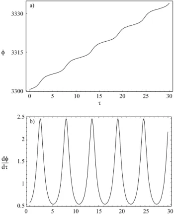
β. Therefore, by a first order solution inβ of the sta-tionary portion of Eq. (11), we find φmax = π2 and mmaxA ≈ 2β. Plots of the time evolution of the angu-lar variable φand its derivative, found by numerically integrating Eq. (11), are shown in Figs. 3a and 3b, respectively, for β = 0.1 andmA = 0.3> mmaxA ≈0.2.
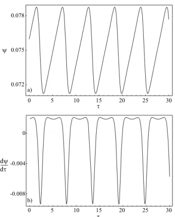
Plots of the time evolution of the angular variable ψ
and its derivative, found by evaluating Eq. (9), on the other hand, are shown in Figs. 4a and 4b, respectively, forβ = 0.1 andmA= 0.3> mmaxA ≈0.2.
We would now like to calculate the time-averaged valuehωiof the angular frequencyω= dφdτas a function of a constant normalized applied torque mA. We have
already noticed thathωi= 0 for−2β 6mA62β. For mA> mmaxA , we solve the differential equation (11) and
then set
U
red
f
15
10
5
0
-5
-10
-15
-10 -5 0 5 10
Figure 2 - Effective reduced potentialUredas a function of
the average angular positionφ forβ= 0.1 and formA= 0
(dotted line),mA= 0.075 (dashed line)andmA= 0.15(full
line).
f 3330
3315
3300
t
0 5 10 15 20 25 30
t
0 5 10 15 20 25 30
d d
f t
2.5
2
1.5
1
0.5 a)
b)
Figure 3 - Time evolution of the angular variableφ(a) and its derivative with respect to time dφ
dτ (b), forβ= 0.1 and
mA= 0.3.
hωi= mA 2β −cos
³mA
4
´
hsinφi −
β
4 sin 2³mA
4
´
hsin 2φi. (19)
In this way, we obtain the hωivs. mA curves
rep-resented in Fig. 5 for three values of the parameter
β (β = 0.05, 0.1, 0.2). We notice that the solution
mmax
4304-4 De Luca
0.078
0.075
0.072 y
t
0 5 10 15 20 25 30
t
0 5 10 15 20 25 30
d d
y t
0
-0.004
-0.008 a)
b)
Figure 4 - Time evolution of the angular variableψ(a) and its derivative with respect to time dψ
dτ (b), forβ= 0.1 and
mA= 0.3.
<
>
w
10
8
6
4
2
0
mA
0 0.2 0.4 0.6 0.8 1
Figure 5 - Time average hωi of the derivative ω = dφ dτ as
a function of the normalized applied torque mA for three
values of the parameter β (from top to bottom:β = 0.05,
β= 0.1andβ= 0.2).
4.
Conclusion
We have shown, by a first order perturbation expan-sion with respect to the parameter β = mglk
T , that the dimensionality of the dynamical equations for two over-damped identical pendulums of mass m and length l, coupled by a massless rod with torsional spring con-stant kT, can be reduced from two to one. Owing to
this reduction, the resulting dynamical equation is writ-ten in terms of the average angular variableφ=φ1+2φ2 and appears to be the same as that of a single pen-dulum with an additional second harmonic sine term. The reduced potential of this mechanical system is seen to be a washboard-like potential, like the one found for a single Josephson junction [1]. The two systems, the mechanical one and the one containing Josephson junc-tions, however, differ in what follows. The mechanical system is forced by an externally applied torque, and this forcing quantity appears as the argument of the cosine and of the sine terms, which are the pre-factors of the sinφand sin 2φterms in the dynamical equation, respectively. In the Josephson junction case, this role is played by an externally applied normalized magnetic flux Ψex, which appears as a second forcing term
be-sides the bias currentiB. In this way, in the case of a d.
c. SQUID, where the two Josephson junctions are cou-pled by an interaction having analogous expression as in the case of the two pendulums studied, the resulting effective dynamical equation is written as follows [3]
dφ
dτ + cos (πΨex) sinφ+ πβsin2(πΨ
ex) sin (2φ) = iB
2 . (20)
Clearly, the role played by the externally applied torque in Eq. (11) is here played, only partially, by the bias current appearing as a forcing quantity in the right hand side of Eq. (20). The magnetic field, on the other hand, plays a complementary role, being the only forc-ing term present in the left hand side of Eq. (20). A last difference can be noticed in the absence of the per-turbation parameterβ in the denominator of the right hand side forcing term in Eq. (20), as opposed to the presence of this parameter in the homologous position in Eq. (11).
Acknowledgments
The author would like to thank Dr. Francesco Romeo for having inspired the present work with his constant dedication to finding new ways of approaching solved and unsolved problems.
References
[1] A. Barone and G. Patern`o, Physics and Applications of the Josephson Effect (Wiley, New York, 1982).
[2] S.H. Strogatz, Nonlinear Dynamics and Chaos
(Perseus Publishing, Cambridge, 2000).