Claudio R. Lucinda
Resumo
Neste artigo, o objetivo é rever os testes empíricos existentes para o grau de competição no setor bancário brasileiro, assim como propor algumas alternativas. Após a descrição do ambiente institucional do sistema bancário brasileiro, os testes sobre a competição, presentes na literatura, foram revisados, começando com o proposto por Panzar e Rosse (1987). A principal conclusão que pode ser extraída desta análise é que o mercado não aparenta estar em equilíbrio de longo prazo, indicando que o mercado não é regido por condições de colusão perfeita. O passo seguinte foi tentar uma nova metodolodia aplicada por Moreno, Martínez e Ruiz (2006) para o mercado bancário espanhol. Nesta metodologia, em que a hipótese de igualdade dos parâmetros de conduta entre empresas e ao longo do tempo é relaxada, os resultados indicam que, para algumas empresas e em alguns instantes do tempo, uma conduta coo-perativa está presente.
Palavras-Chave competição bancária
Abstract
The aim of this paper is to review some of the existing tests for competition in Brazilian banking, as well as to propose an alternative. After the description of the institutional setting of the Brazilian Banking system on this period, the competition tests on the literature were reviewed, beginning with the test proposed by Panzar and Rosse (1987). The market does not seem to be in long-run equilibrium, implying only the market does not seem to find itself in collusive outcome. The next step was to try a new methodology, applied by Moreno, Martínez and Ruiz (2006) for the Spanish banking market. On this methodology, in which the assumption of equality of conduct parameters between firms and time periods is relaxed, the results indicate that, for some firms and in some time periods, a cooperative conduct in fact is present.
Keywords banking competition
JEL Classiication L13, L11
Faculdade de Economia, Administração e Contabilidade de Ribeirão Preto, Universidade de São Paulo (FEA-RP/USP). E-mail: [email protected].
1
Introduction
Since the Real Stabilization Plan of July 1994, one of the most important research questions facing the academic community is about the interest rate charged by the bakning system. As of March 2010, from an interest rate of about 8.75% per annum on Brazilian Treasury bonds, the lending interest rate reaches from 30.45% p.a. in the case of Working Capital Loans, to 161.05% p.a. in the case of overdraft accounts to individuals. Furthermore, the data also show the Brazilian economy is characterized by a low degree of financial intermadiation. According to Belaisch (2003), the Brazilian banking system is surprisingly small, compared to industria-lized economies. The importance of these styindustria-lized facts was not left unattended of the professional academic community in Brazil, the literature on this subject is growing steadily, and can be categorized on three strands. The first one emphasi-zes the role of institutional elements on the lending rates' spread over the risk-free rates. Some of the most important elements singled out for analysis are:
• The role the tax code currently plays on the intermediation spread between lending and borrowing. On this subject, Cardoso and Koyama (2000) report on taxes and contributions currently levied on the lending operations by banks, which were then responsible for approximately 17,1% of the lending rate on a two month lending operation for a company.
• The reduced creditor protection offered by Brazilian law, associated with the high levels of non-performing credits on the portfolios of banks. The same study of Cardoso and Koyama (2000) also indicates the high amount of non-perfor-ming loans increases significantly the spread, which can only be reduced by increased credit information and improvements on creditors' rights. This line of reasoning is also present on papers by Costa (2004) and Costa and Nakane (2004).
Finally, the last line of research enphasizes the role of competition on the deter-mination of spreads. On this subject, Belaisch (2003)used a panel database to conclude that the behavior of a sample of Brazilian banks is not consistent with a competitive market structure. Other important papers on the subject are Nakane (2001, 2004), and Petterini and Jorge Neto (2003), which use econometric te-chniques to determine if the behavior of Brazilian banks is consistent with some alternative competition structures.
Petterini and Jorge Neto (2003) use a version of the model by Jaumandreu and Lorences (2002), and conclude for the rejection of the collusive hypothesis on the Brazilian banking industry. A two step approach was used, in which are estimated demand equations in a first step in order to obtain the relevant own and cross price elasticities. Given those elasticities, the results corresponding to differing equilibria are computed and a model selection test statistic is used for selecting the behavior not rejected by the evidence presented by the data.
Nakane (2001) uses the methodology presented in Bresnahan (1982) and Lau (1982) to estimate the percentage response of the market supply of loans to a gi-ven percentage change on the loan supply of a gigi-ven bank. The estimated value by Nakane (2001) is significantly different from zero, indicating the rejection of the perfect competition hypothesis. However, the small magnitude of the coefficient, combined with the results of statistical tests, also point out to the rejection of the collusion hypothesis.
Using the Panzar and Rosse (1987) methodology, Belaisch (2003) finds evidence of a non-competitive market strutucture. Araújo et al. (2005) also use this metho-dology as a stepping stone on their analysis of the effects of market concentration on competition, and also report results consistent with Belaisch's (2003). All these results do have some similarities, for in all of them the hypotheses of a behavior consistent with either extreme of the taxonomy of market strutuctures – perfect competition or monopoly – is rejected by the data. Even though this result does shed some light on the matter, it still does not give evidence on how Brazilian banks compete.
2
History and Institutional Characteristics of the Brazilian Banking Sector
In order to better understand the characteristics of the Brazilian banking system one must begin by highlighting the effects of the high inflation environment that was a fixture of the Brazilian economy from the beginning of the eighties to the successful stabilization plan (Real Plan) in 1994.1 According to Loyola et al. (2003), the most important characteristics, were:
• Overbranching: the race for deposits in the period of high inflation entailed the opening of a large number of branches, many of which were not profitable after the Real Plan.
• Overbanking: the high inflation period also witnessed the opening of a large number of banking institutions, reaching 250 in 1993, from 121 in 1987.
• Collapse of the long-run credit market: given the high level and variability of the inflation rates, Brazilian banks refrained from their classical functions of channeling credit and financial intermediation.
• High level of investment of information technology and clearing of payments, given the need for a speedy clearing of outstanding inter-bank balances.
After the Real Plan, the sudden decrease on the inflation rates, by reducing the revenues associated with the management of the short-run deposits, exposed some of the operational problems of these institutions. The most affected group was composed of state owned banks, and specially the ones owned by subnational go-vernments, which were used as quasi monetary authorities by the state governors,2 as well as a source of political benefits for the incumbent political party. On the second half of the nineties, these practicies had to end, exposing the weak operatio -nal performance of such banks. This led to the restructuring of the sector, helped by a program designed by the Federal Government (PROES).3
1 One of the most interesting characteristics of the Brazilian inflationary process was the lack of an overt process of dollarization, as in the other Latin American countries during the same period. The agents responded to the high inflation environment by moving their resources to the banking system, which developed a large number of financial instruments intended to protect the real
value of money holdings. Despite being interesting, this will not be our aim on this paper, except
where it provides a backdrop for some institutional characteristics of the system.
2 Before the Stabilization Plan, the state governors used to finance their expenditures through
their banks, which regularly turned insolvent. However, the Federal Government usually ended up bailing out these banks, warranting their use as independent monetary authorities.
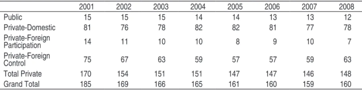
However, not only the state owned banks found themselves with difficulties after the decrease in inflation rates. For the private owned banks, the federal government also set up a program to ease the restructuring of such banks, denoted PROER.4 This program, which made available credit lines for the prospective buyers and allo-wed the break-up of the troubled banks into two parts,5 enabled a relatively quick turnover of the banks affected by the disinflation process. The following table gives some details on the structure and evolution of the banking system:
Table 1 – Brazilian Banking Industry – Selected Indicators
2001 2002 2003 2004 2005 2006 2007 2008 Public 15 15 15 14 14 13 13 12 Private-Domestic 81 76 78 82 82 81 77 78 Private-Foreign
Participation 14 11 10 10 8 9 10 7 Private-Foreign
Control 75 67 63 59 57 57 59 63 Total Private 170 154 151 151 147 147 146 148 Grand Total 185 169 166 165 161 160 159 160 Source: Central Bank of Brazil.
As regards prices of the services offered by the Brazilian Banking System, in January 2010, the spreads over the basic were about 120 to 140 percentage points in the case of overdraft accounts, to less than 40 percentage points for personal credit lines and 20 p.p. to auto credit. For businesses, the spreads seem to be more vola-tile, ranging from 50 p.p. in discounts of trade notes to less than 10 p.p. in vendor credit. The next step in the analysis is to investigate the nature of the competition on the Brazilian Banking System.
3
Competition on Brazilian Banking System
After discussing the institutional characteristics of the Brazilian Banking Sector on the previous one, the empirical evaluation of the behavior of the system is carried out. In order to carry out such a challenge, a database from quarterly balance sheet data from the first quarter of 2000 to the fourth quarter of 20056 was
assem-4 In Portuguese, Programa de Estímulo à Reestruturação e ao Fortalecimento do Sistema Financeiro Nacional.
5 The troubled banks were split into two parts. One included the non-performing assets, and was handed over to the Central Bank for recovery of such credits and repayment to the shareholders and some creditors. The second part, which included the portfolio of "good'' credits and the deposits, was to be auctioned off.
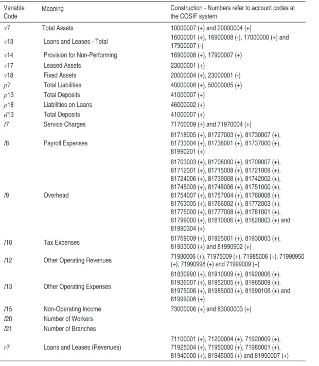
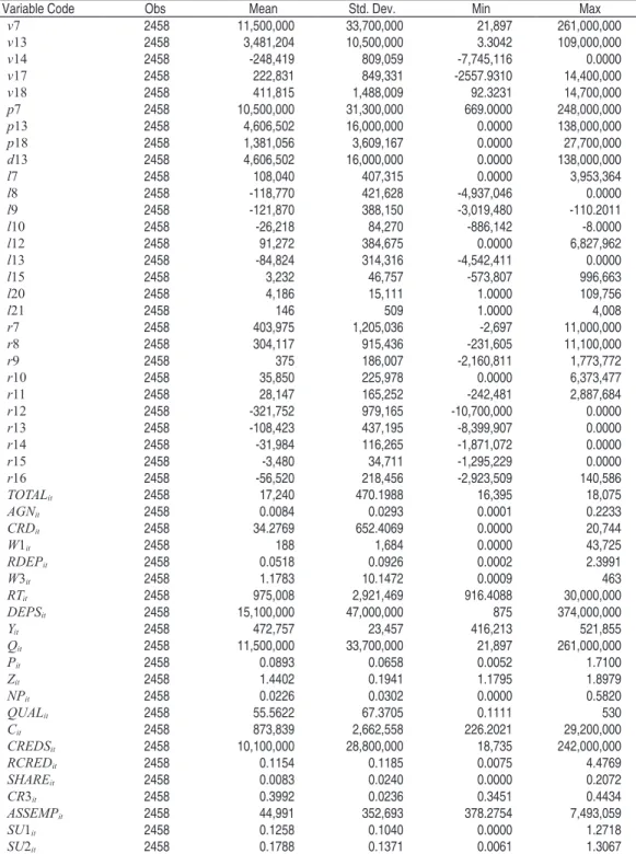
bled. For each of the banks, data on assets, liabilities and net profit statement was collected, and the relevant variables for the econometric analysis that follows are constructed. The definition of the variables is presented below, and the descriptive statistics are presented on the Appendix A.
Table 2 – Variable Deinitions
Variable Code
Meaning Construction - Numbers refer to account codes at the COSIF system
v7 Total Assets 10000007 (+) and 20000004 (+)
v13 Loans and Leases - Total 16000001 (+), 16900008 (-), 17000000 (+) and 17900007 (-)
v14 Provision for Non-Performing 16900008 (+), 17900007 (+)
v17 Leased Assets 23000001 (+)
v18 Fixed Assets 20000004 (+), 23000001 (-)
p7 Total Liabilities 40000008 (+), 50000005 (+)
p13 Total Deposits 41000007 (+)
p18 Liabilities on Loans 46000002 (+)
d13 Total Deposits 41000007 (+)
l7 Service Charges 71700009 (+) and 71970004 (+)
l8 Payroll Expenses
81718005 (+), 81727003 (+), 81730007 (+), 81733004 (+), 81736001 (+), 81737000 (+), 81990201 (+)
l9 Overhead
81703003 (+), 81706000 (+), 81709007 (+), 81712001 (+), 81715008 (+), 81721009 (+), 81724006 (+), 81739008 (+), 81742002 (+), 81745009 (+), 81748006 (+), 81751000 (+), 81754007 (+), 81757004 (+), 81760008 (+), 81763005 (+), 81766002 (+), 81772003 (+), 81775000 (+), 81777008 (+), 81781001 (+), 81799000 (+), 81810006 (+), 81820003 (+) and 81990304 (+)
l10 Tax Expenses 81769009 (+), 81925001 (+), 81930003 (+), 81933000 (+) and 81990902 (+)
l12 Other Operating Revenues 71930006 (+), 71975009 (+), 71985006 (+), 71990950 (+), 71990998 (+) and 71999009 (+)
l13 Other Operating Expenses
81830990 (+), 81910009 (+), 81920006 (+), 81936007 (+), 81952005 (+), 81965009 (+), 81975006 (+), 81985003 (+), 81990108 (+) and 81999006 (+)
l15 Non-Operating Income 73000006 (+) and 83000003 (+)
l20 Number of Workers
l21 Number of Branches
r7 Loans and Leases (Revenues)
Variable Code
Meaning Construction - Numbers refer to account codes at the COSIF system
r8 Repo-Resell (Revenues)
71400000 (+), 71500003 (+), 71580009 (-), 71940003 (+), 71945008 (+), 71947006 (+), 71990053 (+), 71990101 (+), 71990156 (+), 71990204 (+), 71990709 (+), 81500000 (+), 81550005 (-), 81830055 (+), 81830103 (+), 81830158 (+), 81830206 (+) and 81830701 (+)
r9 Derivative Financial Instruments (Revenues) 71580009 (+), 81550005 (+), 71990266 (+) and 81830268 (+)
r10 Foreign Exchange (Revenues) 71300007 (+) and 81400007 (+) (if positive)
r11 Required Deposits (Revenues) 71955005 (+), 71960007 (+), 71965002 (+), 71990125 (+) and 81830127 (+)
r12 Deposits, Acceptances and Repo-Repurchases
(Expenses) 81100008 (+) and 81980008 (+)
r13 Borrowing (Expenses) 81200001 (+) and 81960004 (+)
r14 Lease (Expenses) 71990503 (+), 81300004 (+), 81830505 (+) and 81830550 (+)
r15 Exchange Rate Operations (Expenses) 71300007 (+) and 81400007 (+) (if negative)
r16 Allowance for Bad Credits
71990307 (+), 71990352 (+), 71990400 (+), 71990606 (+), 81830309 (+), 81830354 (+), 81830402 (+) and 81830608 (+)
TOTALit Total Number of Branches in the System (Per Quarter)
AGNit Share of Total Number of Branches l21/TOTALit
CRDit Risk on Financial Intermediation v13/(d13 + p18)
W1it Payments to the Labor Force (-l8/l20)
RDEPit Remuneration to deposits ((-1)*(r12 + r13 + r14 + r15 + l13))/(p7 + p13)
W3it Remuneration fo Physical Capital (-l9)/(v17+v18)
RTit Total Revenue (r7+r8+r9+r10+r11+l7+l12+l15)
DEPSit Total Deposits (p7+p13)
Yit GDP at Market Prices (Source:IPEA)
Qit Total Assets v7
Pit Ratio of Annual Interest Income to Total Assets (r7+r8+r9+r10+r11)/v7
Zit Interbank Rate - Per Quarter (Source: IPEA and transformation to per quarter)
NPit Share of Non-Performing Assets (-1)*(v14/v7)
QUALit Measure of Quality of services l20/l21
Cit Total Costs
(-1)*(l8+l9 + l10 + l13 + r12 + r13 + r14 + r15+ r16)
CREDSit Total Credits v8 + v9 + v10 + v13 + v15
RCREDit Remuneration to credits (r7 + r8 + r9 + r10 + r11 + l7 + l12)/CREDSit
SHAREit Market Share in Credits
CR3it Sum of the three largest market shares
ASSEMPit Assets per Employee v7/l20
SU1it
Share of Remuneration of Employees in Total
Cost (-1)*(l8)/Cit
SU2it
Share of Remuneration of Physical Capital in
A definite conclusion on how Brazilian banks compete must require answers to some questions before any econometric test is carried out. One of the most impor-tant questions is about the definition of the relevant variables, since there is some disagreement on what consititute inputs and outputs of the banking activity. For instance, in some papers the deposits are considered as an input for the produc-tion of the output – as in the "Monti-Klein'' model of financial intermediaproduc-tion.7 In others, both credits and deposits are services to be considered as outputs to be offered in joint production. In order to consider all possibilities, we will adopt an ecletic approach, allowing both possibilities.8
As for the methodological approaches followed here, we chose options based on the estimation of conduct parameter – either directly or as a measure that can bem mapped in the conduct parameter such as Panzar and Rosse (1987) . Alternative approaches, such as of the non-nested hypothesis favored by Nevo (1998) are not possible because of the lack of avaliable data.
3.1 he Panzar-Rosse Methodology
For analyzing Brazilian banking competition, the first econometric test is based on the general methodology proposed by Panzar and Rosse (1987) for what they call "monopoly equilibrium''. On that paper, they start from the comparative statics of a firm's equilibrium under alternative competition assumptions. From that point on, they derive conclusions on the sum of the elasticities of the total revenue with respect to the prices of each of the productive factors, which they denote ψ and the following literature calls the "Statistic H of Panzar and Rosse''. The conclusions are stated as follows:
• Theorem 1 (Panzar and Rosse, 1987, p. 445): "The sum of the factor price elas-ticities of a monopolist's reduced form revenue equation9 must be nonpositive.'' (thus, ψ ≤ 0).
• Proposition 1 (Panzar and Rosse, 1987, p. 451): "In symmetric Chamberlinian equilibrium, the sum of the elasticities of firm's reduced form revenues with respect to factor prices is less than or equal to unity.'' (thus, ψ ≤ 1).
7 It is important to notice, though, the assumption of deposits as an independent product does not imply the deposits of an individual bank cannot be used to increase the supply of an individual bank. The deposits, even though they are considered a service provided to its customers, are used
to finance the interbank market which is the source of all loans. An useful reference is Freixas
and Rochet (1997), p. 55.
8 The financial institutions selected were both commercial banks, which were able to finance themselves by deposits and investment banks, which were not.
9 Reduced form revenue equation means the equation on which the total revenue is a function of
• Proposition 2 (Panzar and Rosse, 1987, p. 452): "For firms observed in long-run competitive equilibrium, the sum of the elasticities of reduced form revenues with respect to factor prices equals unity.'' (thus, ψ = 1).
The meaning of Proposition 2 could be interpreted as follows (SHAFFER, 2004): in an industry in the long-run competitive equilibrium, all firms are operating at the minimum efficient scale. In response to a given increase on input prices, and supposing the cost function to be homogeneous of degree one in factor prices, the average cost increase will be by the same percentage amount as the original increase in input prices. This change in the cost function will lead to entry or exit, giving way to a different equilibrium. On this new equilibrium, the quantity demanded is unchanged, but the price is not; since companies are producing at the minimum average cost on the new cost curve, this means the revenues have increased by the same amount. Thus, the effect of an increase in input prices is to bring about an increase in total revenue by the same percentage amount.
The Theorem 1 could be understand as follows: in a monopoly equilibrium, the quantity supplied is such to equate the marginal revenue to marginal cost. Supposing the marginal cost function homogeneous of degree one again, and the marginal cost curve to intersect the marginal revenue curve from below, the res-ponse of a monopolist to an increase in input prices is an increase in marginal cost by the same percentage amount as the increase in factor prices, and a decrease in quantities. Since marginal revenue is always non-negative in equilibrium, this means the total revenue must decrease, implying ψ ≤ 0.
The authors also try to investigate the behavior of this statistic under the assump-tion of a conjectural variaassump-tions oligopoly, but they find out the behavior of ψ on this case to be indeterminate. The only result these authors derive refers to the effect of factor prices on output.10
This methodology has been applied in many settings, besides the applications by Araújo et al. (2005) and Belaisch (2003) for the Brazilian banking. Mathisen and Buchs (2005) also apply it for the Ghanian financial system, Prasad and Ghosh (2005) do the same for the Indian Banking system, Bikker and Raaf (2002) for the the european banking sector, among many others.11 Cetorelli (1999) has a short survey of the most important methodologies.
10 They found out the sum of elasticites of factor prices on the reduced form output equation is to be negative
However, this methodology is not exempt of problems. The first one is that the results derived by Panzar and Rosse (1987) are found under conditions of long-run equilibrium only. If this condition is not verified in practice, the Panzar and Rosse statistic has its meaning changed. As Shaffer (1983) have pointed out, in the case of short-run equilibrium the test on the ψ statitsic reduces to an one tailed test in which a positive value rejects any form of imperfect competition, and a negative value is consistent with various possible competitive structures. This test of long-run competition is usually carried out by investigating the effects of changes in input prices on profits. Is these are zero, it is assumed the market is in long-run equilibrium.
The second problem is some test results might not discriminate between different market structures. As Panzar and Rosse (1987, p. 451) state after deriving the range of values consistent with the Chamberlinian oligopoly:
The range of permissible values for ψ – i.e., the values for the H
statistic consistent with Chamberlinian equilibrium – includes
that of ψ*– the values for the H statistic consistent with
Monopoly equilibrium – (i.e., the negative real line) plus the unit
interval. Thus the analyst can, in principle, observe data that are consistent with the hypothesis of monopolistic competition but
not with that of profit maximizing monopoly.
As Shaffer (1983, 2004) also points out, a value for ψ equal to one could be consistent with either a policy of fixed markups or a sales maximization under a break-even constant, or even in a market of local natural monopolies under contestability.
Another criticism comes from Bikker et al. (2006), which conclude the inclusion of scale variables as independent regressors in the Panzar-Rosse test equation tends to bias the ψˆ coefficient upward.
In any case, this methodolgy provides a useful starting point, since this methodolo-gy doees not require defining the relevant markets, and our application of the test is based upon the following regression:
ln(RTit) = β1ln(AGNit) + β2ln(CRDit) + β3ln(DEPSit) +
In which the term fi denotes the individual effect and the Panzar-Rosse H statistic
is β4 + β5 + β6. The AGNit variable, defined as in Araújo et al. (2005) as the share
of bank i in the systemwide number of branches, is related to the "too big to fail'' characteristic that some banks present. The CRDit variable, total loans over the sum
of total deposits and liabilities on loans, was intended as a proxy for intermediation risk; and DEPSit, total deposits, tries to capture scale economies.
The RDEPSit, W1it and W3it variables are the input prices in this case (deposits,
payments to the labor force and remuneration to physical capital), meaning we are implicitly adopting the view of the banking firm as of the "Monti-Klein'' model. The results are presented both for the full sample, as well as for sub-samples comprising only commercial banks, investment banks and sub groups sorted according to size (banks with average assets below 250 million Reais, those with assets between 250 and 5,000 and those with average assets above 5,000 million reais).12 Another interesting issue13 is that many mergers happened during this period. In order to face the effect of these mergers on the results, the estimates were also carried out using only the balanced sample, that is, banks which were present at all time periods in our sample.
12 The smaller group comprises banks associated with retailers, smaller brokerage firms and bran-ches of international groups. The medium sized institutions were banks associated with auto-makers (such as GM, Volkswagen) and former regional state owned banks. And finally, the largest group comprises the largest private banks, as well as Banco do Brasil and CEF, as well as some of the larger subnational state owned banks.
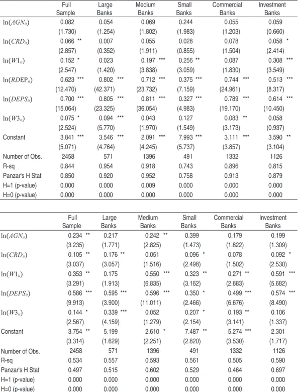
Table 3 – Regression Results – Deposits as an Input (Top)
Full Sample
Large Banks
Medium Banks
Small Banks
Commercial Banks
Investment Banks
ln(AGNit) 0.082 0.054 0.069 0.244 0.055 0.059
(1.730) (1.254) (1.802) (1.983) (1.203) (0.660)
ln(CRDit) 0.066 ** 0.007 0.055 0.028 0.078 0.058 *
(2.857) (0.352) (1.911) (0.855) (1.504) (2.414)
ln(W1it) 0.152 * 0.023 0.197 *** 0.256 ** 0.087 0.308 ***
(2.547) (1.420) (3.838) (3.059) (1.830) (3.549)
ln(RDEPit) 0.623 *** 0.802 *** 0.712 *** 0.375 *** 0.744 *** 0.513 ***
(12.470) (42.371) (23.732) (7.159) (24.961) (8.317)
ln(DEPSit) 0.700 *** 0.805 *** 0.811 *** 0.327 *** 0.789 *** 0.614 ***
(15.064) (23.325) (36.054) (4.983) (19.170) (10.450)
ln(W3it) 0.075 * 0.094 *** 0.043 0.127 0.083 ** 0.058
(2.524) (5.770) (1.970) (1.549) (3.173) (0.937) Constant 3.841 *** 3.546 *** 2.091 *** 7.993 *** 3.111 *** 3.590 **
(5.071) (4.764) (4.245) (5.737) (3.857) (3.104) Number of Obs. 2458 571 1396 491 1332 1126 R-sq 0.844 0.954 0.918 0.743 0.896 0.815 Panzar's H Stat 0.850 0.920 0.952 0.758 0.913 0.879 H=1 (p-value) 0.000 0.000 0.009 0.000 0.000 0.000 H=0 (p-value) 0.000 0.000 0.000 0.000 0.000 0.000
Full Sample
Large Banks
Medium Banks
Small Banks
Commercial Banks
Investment Banks
ln(AGNit) 0.234 ** 0.217 0.242 ** 0.399 0.179 0.199
(3.235) (1.771) (2.825) (1.473) (1.822) (1.309)
ln(CRDit) 0.105 ** 0.176 ** 0.051 0.096 * 0.078 0.092 *
(3.037) (3.057) (1.516) (2.498) (1.502) (2.530)
ln(W1it) 0.353 ** 0.175 0.550 *** 0.323 ** 0.271 ** 0.591 ***
(3.291) (1.913) (6.835) (3.162) (2.683) (5.682)
ln(DEPSit) 0.586 *** 0.595 *** 0.596 *** 0.350 * 0.499 *** 0.574 ***
(9.913) (3.900) (11.011) (2.466) (6.676) (8.490)
ln(W3it) 0.144 * 0.339 *** 0.052 0.207 * 0.193 ** 0.106
(2.567) (4.159) (1.279) (2.154) (3.141) (1.337) Constant 3.754 ** 5.199 2.610 * 7.487 ** 5.274 *** 2.301 (3.314) (1.629) (2.251) (2.820) (3.530) (1.717) Number of Obs. 2458 571 1396 491 1332 1126 R-sq 0.534 0.557 0.593 0.561 0.505 0.590 Panzar's H Stat 0.497 0.515 0.602 0.529 0.464 0.697 H=1 (p-value) 0.000 0.000 0.000 0.000 0.000 0.000 H=0 (p-value) 0.000 0.000 0.000 0.000 0.000 0.000
The robust standard errors are in parentheses, and the table points out some in-teresting results. The first one is all variables are highly significant and the model does present a high explanatory power. And finally, the results for the test of competitive structure point out to a Panzar-Rosse H Statistic of 0.8, and both hy-potheses of ψ = 0 and ψ = 1 are rejected, which should point out to a competitive structure of Chamberlinian oligopoly, if the market is shown to be in long-run equilibrium. The results are qualitatively similar for each subsample, in which both hypotheses ψ = 0 and ψ = 1 are rejected.
Two other alternatives were tried, in order to face the criticisms posed by Bikker
et al. (2006) about the inclusion of scale variables as explanatory variables. In one
alternative, the ln(DEPSit) variable was dropped from the estimating equations and in the other alternative both ln(DEPSit) and ln(AGNit) were dropped. In both alter-natives the estimated ψ statistics were higher than at the previous table, at odds to the expected bias described by Bikker et al. (2006); furthermore, the resulting decrease in explanatory power, in some cases, led us to not reject the perfect com -petition hypothesis.
The test was also carried out assuming deposits are not inputs to the banking firm, and the results – which also point out to a rejection of both hypotheses of perfect competition and monopoly – are presented on the bottom panel of Table 3.
Since the results do not seem to be driven by the behavior of any subgroup in our sample neither by scale effects bias such as pointed out by Bikker et al. (2006), the next step was to investigate of the markets can be considered in Long-Run equi -librium. The usual test for this hypothesis, as discussed before, involves the sum of elasticities of factor prices with respect to companies' profits. This test will be carried out by using the following specification
ln(RTit – Cit) = β1ln(AGNit) + β2ln(CRDit) + β3ln(DEPSit) +
+ β4ln(W1it) + β5ln(RDEPSit) + β6ln(W3it) + fi + εit
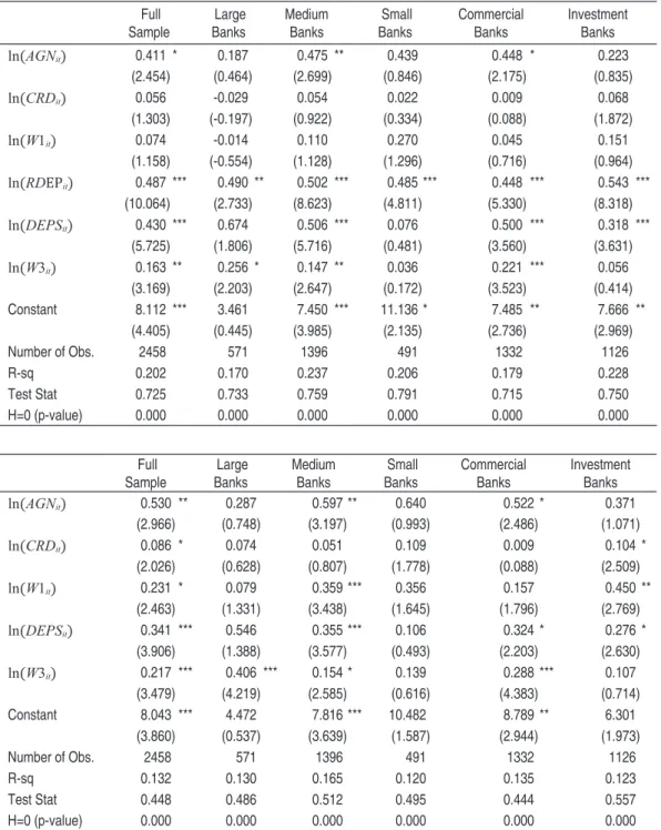
This profit tests for the complete sample and the subsamples discussed previously are on the following table. Alternative specifications without the ln(DEPSit) and
Table 4 – Proit Test – Deposits as an Input (Top)
Full Sample
Large Banks
Medium Banks
Small Banks
Commercial Banks
Investment Banks
ln(AGNit) 0.411 * 0.187 0.475 ** 0.439 0.448 * 0.223
(2.454) (0.464) (2.699) (0.846) (2.175) (0.835)
ln(CRDit) 0.056 -0.029 0.054 0.022 0.009 0.068
(1.303) (-0.197) (0.922) (0.334) (0.088) (1.872)
ln(W1it) 0.074 -0.014 0.110 0.270 0.045 0.151
(1.158) (-0.554) (1.128) (1.296) (0.716) (0.964)
ln(RDEPit) 0.487 *** 0.490 ** 0.502 *** 0.485 *** 0.448 *** 0.543 ***
(10.064) (2.733) (8.623) (4.811) (5.330) (8.318)
ln(DEPSit) 0.430 *** 0.674 0.506 *** 0.076 0.500 *** 0.318 ***
(5.725) (1.806) (5.716) (0.481) (3.560) (3.631)
ln(W3it) 0.163 ** 0.256 * 0.147 ** 0.036 0.221 *** 0.056
(3.169) (2.203) (2.647) (0.172) (3.523) (0.414) Constant 8.112 *** 3.461 7.450 *** 11.136 * 7.485 ** 7.666 **
(4.405) (0.445) (3.985) (2.135) (2.736) (2.969) Number of Obs. 2458 571 1396 491 1332 1126 R-sq 0.202 0.170 0.237 0.206 0.179 0.228 Test Stat 0.725 0.733 0.759 0.791 0.715 0.750 H=0 (p-value) 0.000 0.000 0.000 0.000 0.000 0.000
Full Sample
Large Banks
Medium Banks
Small Banks
Commercial Banks
Investment Banks
ln(AGNit) 0.530 ** 0.287 0.597 ** 0.640 0.522 * 0.371
(2.966) (0.748) (3.197) (0.993) (2.486) (1.071)
ln(CRDit) 0.086 * 0.074 0.051 0.109 0.009 0.104 *
(2.026) (0.628) (0.807) (1.778) (0.088) (2.509)
ln(W1it) 0.231 * 0.079 0.359 *** 0.356 0.157 0.450 **
(2.463) (1.331) (3.438) (1.645) (1.796) (2.769)
ln(DEPSit) 0.341 *** 0.546 0.355 *** 0.106 0.324 * 0.276 *
(3.906) (1.388) (3.577) (0.493) (2.203) (2.630)
ln(W3it) 0.217 *** 0.406 *** 0.154 * 0.139 0.288 *** 0.107
(3.479) (4.219) (2.585) (0.616) (4.383) (0.714) Constant 8.043 *** 4.472 7.816 *** 10.482 8.789 ** 6.301 (3.860) (0.537) (3.639) (1.587) (2.944) (1.973) Number of Obs. 2458 571 1396 491 1332 1126 R-sq 0.132 0.130 0.165 0.120 0.135 0.123 Test Stat 0.448 0.486 0.512 0.495 0.444 0.557 H=0 (p-value) 0.000 0.000 0.000 0.000 0.000 0.000 Obs: Asymptotic t Stats in Parentheses. Codes: P-value<0.01 ***, P-value<0.05 ** and value<0.1.
the rather restrictive assumptions required for the usage of Panzar-Rosse statistic as a competition test are soundly rejected. For the balanced sample, the results were qualitatively similar, pointing out to the rejection of the underlying assumptions of the Panzar-Rosse test. This conclusion also obtained when the scale variables are removed from the test equation for a comparison with the test in accordance to the conclusions of Bikker et al. (2006).
The importance of this fact must not be underestimated, since all previous tests using the Panzar-Rosse methodology did not present the results of the long run equilibrium test, putting in check the conslusions raised by both Araújo et al.
(2005) and Belaisch (2003) concerning the competitive structure of this industry. As for the constructive conclusions of the tests above, one is only able to reject the hypothesis of a joint profit maximizing oligopoly (that is, cartel behavior) by Brazilian banks. However, for more specific conclusions regarding the characteri-zation of competition, a different approach must be tried, the theme of the next section.
3.2 he conjectural variations approach
On this section, an alternative approach is explored to identify the competitive conduct, in which the relevant parameters are understood to reflect the firms' "expectations'' about the reaction of their competitors to increased output. More specifically, the version of Gollop and Roberts (1979) presented in the analysis of Spanish banking by Moreno, Martínez and Ruiz (2006) was developed here.
Their model begins by posing an inverse demand function for loans:
Rt = D(∑iCREDSit)
In which D'(⋅)<0, and indicates the market opportunity cost of credit – Rtat the
time period t – is a decreasing function of the aggregate volume of loans, the sum of CREDSit14 at time period t over all banks denoted i. The lending rate for an
in-dividual bank could be expressed as the sum of the opportunity cost of funds, Rt,
and a bank specific variable which collects the differences in service quality. In a sense, the vit variable could be understood as capturing the product differentiation
aspects of the banking services. Thus, the loan rate charged by each bank could be written as:
RCREDit = Rt + vit
RCREDit = D(∑iCREDSit) + vit
The cost function, on the other hand, could be separated on the following way:
Cit = Zit × CREDSit + c(CREDSit, DEPSit, W1it, W3it)
On the previous equation, Zit is defined as the interbank rate under which additional
funds could also be borrowed in order to increase lending. The c(⋅) function repre-sent the operating costs, depending on factor prices (labor and capital), as well as on scale of loans and deposits. From the definition of economic profit, substitution of the cost function defined previously leads to:
Πi = (RCREDit – Zit) × CREDSit – c(DEPSit, W1it, W3it)
Assuming the strategic variable for banks is the volume of loans, differentiation of the profit function with respect to CREDSit leads to, after reorganization:
1 1
it it it it kt it
k i
it it it
RCRED Z CMg S CREDS v
RCRED D ≠ CREDS RCRED
− − = + ∂ −
ε
∑
∂ In which Sit is the market share of bank i on time period t, εD is the price elasticity
of demand with respect to credit rate –
( )
it
t i
it t
i
CREDS R
CREDS R
∂ ×
∂
∑
∑
. The termkt k i
it
CREDS CREDS ≠
∂ ∂
∑
15 is also known as the conjectural variation expected by bank i (that is, the sum of expected changes on the quantity supplied by the firms' competitors in response to a change on its own quantity).16 Usually not enough degrees of fre-edom for estimating each conjectural variation were available, and it is proposed here a technique to reduce the number of coefficients to be estimated.17 It is im-portant to emphasize, though, that despite the different name, this conjectural variation is the same thing as the conduct parameter discussed above.The technique proposed involves rewriting the summation above in terms of s di-fferent groups, defined by their size (less than 250 milllion BRL in assets, between
15 An important result in the analysis is kt k i kt k i
it it
CREDS CREDS
CREDS CREDS
≠ ≠
∂
∂ =
∂
∑
∂∑
16 Recent criticisms of the concept of conduct parameter include Corts (1998), which indicate any structural change in demand and supply variables would make the identification assumptions suspect. Furthermore, Wolfram (1999), Corts (1998) and Puller (2007) conclude the test might only be used to discriminate between competition, collusion and Cournot Equilibrium. Even so, this diminished interpretation of the conduct parameter is an improvement over the results of the previous section.
250 and 5,000 million and above 5,000 million in assets) leading to the following equation:
(
,)
1
1 s k h k i kt 1
it it it it it
h
it D it it
CREDS
RCRED Z CMg S v
RCRED CREDS RCRED
∈ ≠ = ∂ − − = + −
ε ∂
∑
∑
This equation expressing the conjectural variation can be rewritten in relative terms:
(
)
(
,)
1 ,
ln
1 s k h k i kt 1
it it it it it
kt h k h k i
it D it it
CREDS
RCRED Z CMg S v
CREDS
RCRED CREDS RCRED
∈ ≠ = ∈ ≠ ∂ − − = + −
ε ∂
∑
∑ ∑
The term ln
(
k h k i, kt)
it CREDS CREDS ∈ ≠ ∂ ∂
∑
would be the relative conjectural variation, the expec-ted percentage response to an one million BRL in credit supply by bank i. However, the imposition of a same conjecture for every firm in each category implies that banks closer to each other, but belonging to different groups might possess very different conjectures (GOLLOP; ROBERTS, 1979, p. 316). The solution presented by Gollop and Roberts (1979) and adopted by Moreno, Martínez and Ruiz (2006) was to select some firms as benchmarks. The conjectural variation of each firm with respect to each group will be a weighted average of the conjectural variations for each of the benchmarks.
Thus, the term ln
(
k h k i, kt)
it CREDS CREDS ∈ ≠ ∂ ∂∑
is a parameter to be estimated, jh
β , in which j is
an array composed of two elements – Top or Bottom and the group number. The h is the group to which the reaction refers, so the term 1
1
T
β means the response of the largest firm on the first group to changes in the CREDS variable of the compa-nies in the first group.
For a firm i located between the benchmarks j-1 and j, the
β = β + − β
ihw
i Lih(1
w
i)
Tih , in which Lih
β and Ti h
β are the conjectures of the smallest and largest firms in which bank i is classified. The Wi, on the other hand, is a measure of the distance between
i firm and the smallest firm in the group. Thus, the previous equation can be rewritten as:
(
)
(
)
(
1 1 , (1 ))
1s Lk Tk
it it it it it
kt k h k h
h k h k i
it D it
RCRED Z CMg S v
CREDS w w
RCRED = ∈ ≠ RCRED
− − = + β + − β −
In order to estimate this model, two other points must be addressed. The first one relates to the fact the market shares – the Sit variable – and margins are
simulta-neously determined. This problem was faced by specifying a reduced form equation for the market share of bank i, presented below:
Sit = ψ0+ ψ1CR3SHAREit + ψ2Yit + ψ3ASSEM Pit (2)
The other problem is the marginal cost usually is not directly observed (studies such as of Wolfram (1999)which had quite reliable independent estimates of mar-ginal costs are quite rare). Even considering accounting data, one of the most im-portant characteristics of the New Empirical Industrial Organization models is that marginal cost is not an observable quantity. The cost side of the firms was modeled using a translog specification combined with the input relations derived from Shepard's Lemma. Considering a view of the banking firm in which it provides two services – deposits and credits – and demanding two factors, labor and physical capital, the following system of equations is the cost side of the model:
0 1 2 3
2 2
4 5 1 2
2 2
3 4 5
1 2
ln ln ln ln ln
0.5 (ln ) 0.5 (ln ) ln( 1 ) ln( 3 )
ln( 1 ) ln( 3 ) 0.5 (ln( 1)) 0.5 (ln( 3 ))
ln( ) ln( 1 ) ln(
it it it it it
it it it it
it it it
it it it
C CREDS DEPS CREDS DEPS
CREDS DEPS W W
W W W W
CREDS W CREDS
= α + α + α + α × +
+ α + α + γ + γ +
+γ × + γ + γ +
+δ × +δ 3
4
) ln( 3 ) ln( ) ln( 1 )
ln( ) ln( 3 )
it it it
it it
W DEPS W
DEPS W
× +δ × +
+δ ×
(3)
1 4 3 1 3
1it ln( 1 )it ln( 3 )it ln( it) ln( it)
SU = γ + γ W + γ W +δ CREDS +δ DEPS (4)
2 5 3 2 4
3it ln( 3 )it ln( 1 )it ln( it) ln( it)
SU = γ + γ W + γ W +δ CREDS +δ DEPS (5)
The system of equations (3)-(5), which the SU1 and SU2 variables are the shares of labor and physical capital in total costs, imply the marginal cost of credits as being:
(
1 3ln 4ln( ) 1ln( 1 ) 2ln( 3 ))
it
it it it it it
it
C
CMg DEPS CREDS W W
CREDS
= α + α + α +δ +δ (6)
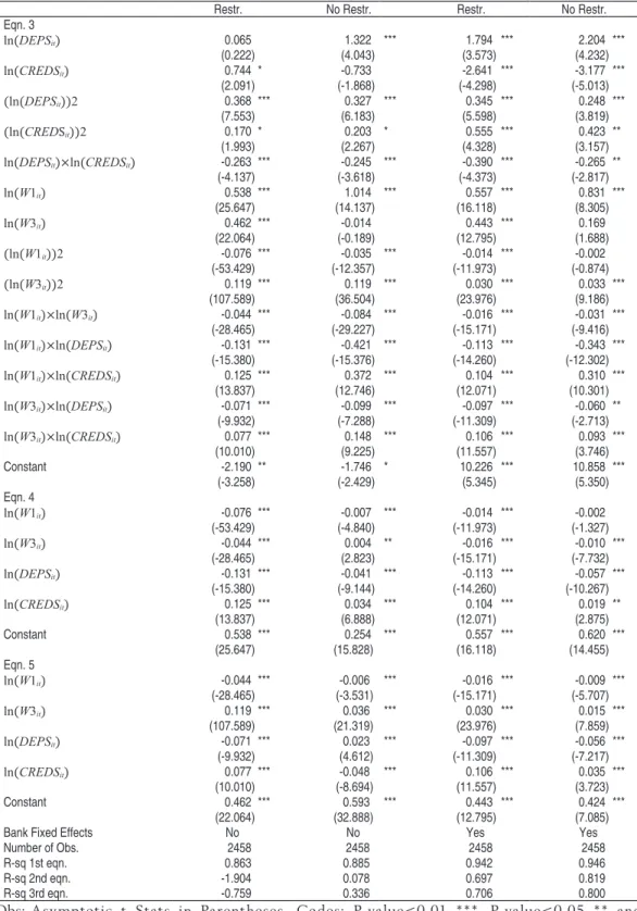
The empirical analysis was carried out in two steps; on the first one the system of equations 3-5 was estimated, and with the coefficients the predicted marginal costs were computed using equation (6). With the predicted marginal costs, the system 1-2 was estimated.18 The estimation method used was the Seemingly Unrelated Regressions system, and the results are on the following tables:
18 The equation (1) was estimated by expanding the parentheses and the vitvariable was approxi
Table 5 – System of Equations (3)-(5)
Restr. No Restr. Restr. No Restr.
Eqn. 3
ln(DEPSit) 0.065 1.322 *** 1.794 *** 2.204 ***
(0.222) (4.043) (3.573) (4.232)
ln(CREDSit) 0.744 * -0.733 -2.641 *** -3.177 ***
(2.091) (-1.868) (-4.298) (-5.013)
(ln(DEPSit))2 0.368 *** 0.327 *** 0.345 *** 0.248 ***
(7.553) (6.183) (5.598) (3.819)
(ln(CREDSit))2 0.170 * 0.203 * 0.555 *** 0.423 **
(1.993) (2.267) (4.328) (3.157)
ln(DEPSit)×ln(CREDSit) -0.263 *** -0.245 *** -0.390 *** -0.265 **
(-4.137) (-3.618) (-4.373) (-2.817)
ln(W1it) 0.538 *** 1.014 *** 0.557 *** 0.831 ***
(25.647) (14.137) (16.118) (8.305)
ln(W3it) 0.462 *** -0.014 0.443 *** 0.169
(22.064) (-0.189) (12.795) (1.688)
(ln(W1it))2 -0.076 *** -0.035 *** -0.014 *** -0.002
(-53.429) (-12.357) (-11.973) (-0.874)
(ln(W3it))2 0.119 *** 0.119 *** 0.030 *** 0.033 ***
(107.589) (36.504) (23.976) (9.186)
ln(W1it)×ln(W3it) -0.044 *** -0.084 *** -0.016 *** -0.031 ***
(-28.465) (-29.227) (-15.171) (-9.416)
ln(W1it)×ln(DEPSit) -0.131 *** -0.421 *** -0.113 *** -0.343 ***
(-15.380) (-15.376) (-14.260) (-12.302)
ln(W1it)×ln(CREDSit) 0.125 *** 0.372 *** 0.104 *** 0.310 ***
(13.837) (12.746) (12.071) (10.301)
ln(W3it)×ln(DEPSit) -0.071 *** -0.099 *** -0.097 *** -0.060 **
(-9.932) (-7.288) (-11.309) (-2.713)
ln(W3it)×ln(CREDSit) 0.077 *** 0.148 *** 0.106 *** 0.093 ***
(10.010) (9.225) (11.557) (3.746) Constant -2.190 ** -1.746 * 10.226 *** 10.858 ***
(-3.258) (-2.429) (5.345) (5.350)
Eqn. 4
ln(W1it) -0.076 *** -0.007 *** -0.014 *** -0.002
(-53.429) (-4.840) (-11.973) (-1.327)
ln(W3it) -0.044 *** 0.004 ** -0.016 *** -0.010 ***
(-28.465) (2.823) (-15.171) (-7.732)
ln(DEPSit) -0.131 *** -0.041 *** -0.113 *** -0.057 ***
(-15.380) (-9.144) (-14.260) (-10.267)
ln(CREDSit) 0.125 *** 0.034 *** 0.104 *** 0.019 **
(13.837) (6.888) (12.071) (2.875) Constant 0.538 *** 0.254 *** 0.557 *** 0.620 ***
(25.647) (15.828) (16.118) (14.455)
Eqn. 5
ln(W1it) -0.044 *** -0.006 *** -0.016 *** -0.009 ***
(-28.465) (-3.531) (-15.171) (-5.707)
ln(W3it) 0.119 *** 0.036 *** 0.030 *** 0.015 ***
(107.589) (21.319) (23.976) (7.859)
ln(DEPSit) -0.071 *** 0.023 *** -0.097 *** -0.056 ***
(-9.932) (4.612) (-11.309) (-7.217)
ln(CREDSit) 0.077 *** -0.048 *** 0.106 *** 0.035 ***
(10.010) (-8.694) (11.557) (3.723) Constant 0.462 *** 0.593 *** 0.443 *** 0.424 ***
(22.064) (32.888) (12.795) (7.085) Bank Fixed Effects No No Yes Yes Number of Obs. 2458 2458 2458 2458 R-sq 1st eqn. 0.863 0.885 0.942 0.946 R-sq 2nd eqn. -1.904 0.078 0.697 0.819 R-sq 3rd eqn. -0.759 0.336 0.706 0.800
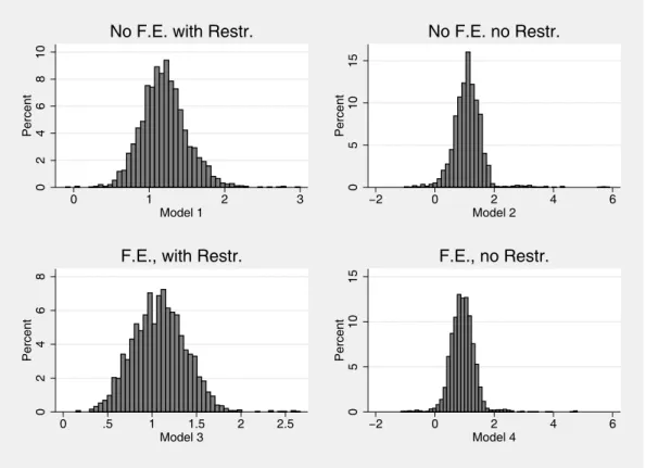
The cost side equation was estimated in four different ways, depending if the cross-equation restrictions were imposed19 and whether firm specific effects were tried, leading to the four versions presented in the previous page. As a further check on the economic plausibility of the results, the implied markups over marginal costs were computed and the distribution is as follows:20
0 2 4 6 8 1 0 Pe rce n t
0 1 2 3
Model 1 No F.E. with Restr.
0 5 1 0 1 5 Pe rce n t
−2 0 2 4 6
Model 2 No F.E. no Restr.
0 2 4 6 8 Pe rce n t
0 .5 1 1.5 2 2.5
Model 3 F.E., with Restr.
0 5 1 0 1 5 Pe rce n t
−2 0 2 4 6
Model 4 F.E., no Restr.
Figure 1 – Distribution of Markups
19 The homogeneity and symmetry restrictions, δ = 0, γ3+ γ4+ γ5= 0 and γ1 + γ2 = 1, were imposed in all alternatives.
20 An important point is related to the estimation of the price elasticity of demand. The approach pursued here was based on Shaffer (1993) and starts by posing the following demand function for banking services – understood as banking assets:
0 1 2 3 4 5
6 7 8 9
10
it it it it it it it
it it it it it it it it it it dit
Q a a P a Y a QUAL a Z a P Y
a P Z a P QUAL a Y Z a Y QUAL
a Z QUAL
= + + + + + × +
+ × + × + × + × +
+ × + ε
(7)
In this demand function, Zit is considered a measure of price of substitutes – since we are
con-sidering the sole output of the banking firm as their assets, this should be analugous to the op-portunity cost of internally generated funds for the firm which demands credits. On the other hand both Yit(proxy for income) and QUALit(proxy for quality of services) are demand shifters.
The estimated markups obtained after imposing the symmetry and homogeneity tended to present similar averages to the estimates without such restrictions, and lower variance of markups.21 Given the estimates of the marginal costs, the pricing side of the model could be estimated. Due to problems of multicollinearity, the conduct parameters were estimated in a way only the expected responses of the largest firm on the sample were estimated directly and the other responses were computed as differences:
Table 6 – System of Equations 1-2
Model 1 Model 2 Model 3 Model 4 Eqn. 1
1 1 1 1 L T
β − β -1.835 -1.817 -1.909 -1.862
(-1.717) (-1.695) (-1.782) (-1.729)
1 1 T
β 1.926 ** 1.910 ** 1.969 ** 1.939 ** (2.853) (2.821) (2.912) (2.850)
1 2 1 1 T T
β + β -1.899 ** -1.883 ** -1.942 ** -1.911 **
(-2.813) (-2.781) (-2.871) (-2.810)
1 3 1 1 T T
β + β -1.926 ** -1.911 ** -1.970 ** -1.939 **
(-2.854) (-2.822) (-2.912) (-2.851)
1 1 2 2 L T
β − β 0.030 0.030 0.030 0.030
(1.609) (1.594) (1.593) (1.572)
1 2
T
β -0.028 * -0.028 * -0.028 * -0.028 * (-2.522) (-2.506) (-2.485) (-2.466)
1 2
2 2
T T
β + β 0.028 * 0.027 * 0.027 * 0.027 *
(2.482) (2.466) (2.446) (2.426)
1 3
2 2
T T
β + β 0.028 * 0.028 * 0.027 * 0.027 *
(2.503) (2.488) (2.467) (2.447)
1 1
3 3
L T
β − β 0.002 0.002 0.002 0.002
(0.487) (0.479) (0.536) (0.511)
1 3
T
β -0.005 * -0.005 * -0.005 * -0.005 * (-2.059) (-2.039) (-2.104) (-2.065)
1 2
3 3
T T
+
β β 0.004 * 0.004 * 0.005 * 0.005 * (2.015) (1.994) (2.059) (2.020)
1 3
3 3
T + T
β β 0.005 * 0.005 * 0.005 * 0.005 * (2.054) (2.033) (2.099) (2.060)
2 2
1 1
L T
β − β -0.051 *** -0.051 *** -0.052 *** -0.052 ***
(-3.765) (-3.760) (-3.780) (-3.774)
2 2
2 2
L T
β − β 0.000 0.000 0.000 0.000
(1.383) (1.406) (1.331) (1.357)
2 2
3 3
L T
β − β 0.000 *** 0.000 *** 0.000 *** 0.000 ***
(3.536) (3.491) (3.619) (3.569)
3 3
1 1
L T
β − β 0.003 0.003 0.003 0.003
(1.698) (1.716) (1.760) (1.773)
3 3
2 2
L T
β − β 0.000 0.000 0.000 0.000
(0.147) (0.167) (0.169) (0.183)
3 3
3 3
L T
β − β 0.000 0.000 0.000 0.000
(0.766) (0.738) (0.750) (0.725) Eqn. 2
CR3SHAREit 0.046 * 0.046 * 0.046 * 0.046 * (2.175) (2.177) (2.169) (2.168)
Yit -0.000 -0.000 -0.000 -0.000 (-1.189) (-1.170) (-1.151) (-1.143)
ASSEMPit -0.000 -0.000 -0.000 -0.000 (-0.480) (-0.448) (-0.489) (-0.459) Constant 0.004 0.003 0.003 0.003
(0.241) (0.227) (0.213) (0.210) Number of Obs. 2458 2458 2458 2458 R-sq 1st eqn. 0.395 0.395 0.401 0.400 R-sq 2nd eqn. -0.002 -0.002 -0.002 -0.002
Obs: Asymptotic t Stats in Parentheses. Codes: P-value<0.01 ***, P-value<0.05 ** and P-value<0.1 *.
For the Model 1, without fixed effects and restrictions, the estimated conduct parameters for a given quarter and their confidence intervals are presented on the following figure:22
0.091 1.926
0.002
−0.028 −0.003−0.005
0
.5
1
1
.5
2
C
o
n
d
.
Pa
ra
me
te
r
1 2 3
L T L T L T
Banks Group 1
−3.876−3.825
0.056 0.056 0.056 0.056
−4
−3
−2
−1
0
C
o
n
d
.
Pa
ra
me
te
r
1 2 3
L T L T L T
Banks Group 2
−3.850−3.852
0.056 0.056
−3.852−3.852
−4
−3
−2
−1
0
C
o
n
d
.
Pa
ra
me
te
r
1 2 3
L T L T L T
Banks Group 3
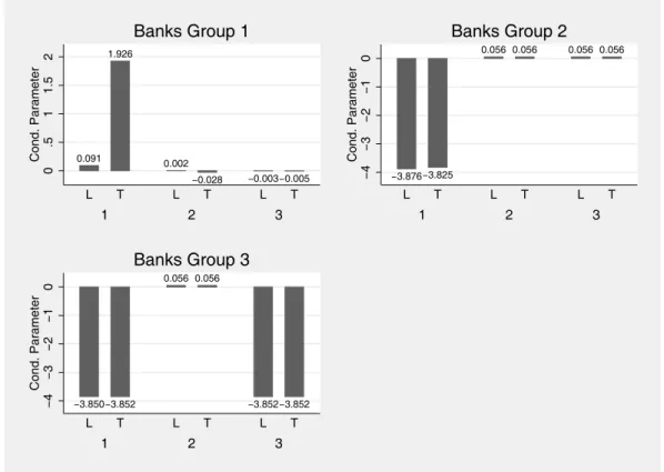
Figure 2 – Estimated Conduct Parameter – 2005/4
Some interesting results in this figure can be inferred. The first one is that there is a great difference between the observed conjectural variations – and by virtue of its definition, also their conduct parameters – for each group. Each of the graphs in the previous table present the response of the reference banks (smallest (L) and largest (T)) with respect to increases in loans by banks in each group.
The resulys in the table point out to firms in group 1 expect an aggressive response by banks in their own group, with their competitors in this group increasing their loan output in response to an increased output, further depressing loan rates. On the other hand, banks in groups 2 and 3 expect a more cooperative response of banks in group 1 to increases in their own output. Banks in group 1 will decrease
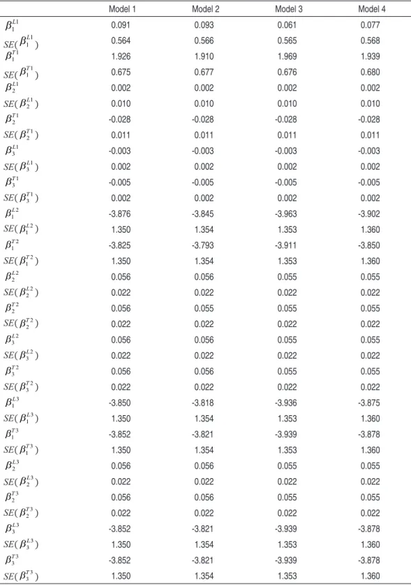
22 Results for the other models – quite similar to the ones presented here – are presented on the
their output in response to increases in loan output by banks in groups 2 and 3, kee-ping the loan rate to decrease further. And finally, in the largest group of banks, the companies expect a cooperative response of their competitors in the same group, reducing their loans after an increase of output by one of them. This also keeps the loan rate from falling.
The estimated conduct parameters, on the other hand, do not lend themselves to an easy mapping to any of the static oligopoly solutions known on the literature. For instance, the standard Cournot oligopoly result would imply firms to react ac-cording to changes in market supply but not acac-cording to the source of the change. This implies firms of different sizes have same expectations of relative responses of rivals – according to Gollop and Roberts (1979), p. 322 –, or all β to be the same and equal to zero, which inspection of the figure above indicates is not the case.
The adequacy of the standard conduct parameter – the approaches of Bresnahan (1982) and Lau (1982) – can also be tested, by the hypothesis all β to be equal, though not necessarily zero, which is also rejected.
Even though the exact competitive assumptions are not revealed by these results, they also point out to another weakness of the Panzar-Rosse (1987) result, which relies on the equality of conduct parameters between firms.
4
Conclusion
In this paper, we tried to review existing tests for competition in the Brazilian banking system and propose some alternatives. The first step in the analysis was to describe the institutional changes after the decrease in inflation rates brought about by the Real Plan in 1994. After the description of the institutional setting of the Brazilian Banking system on this period, the competition tests on the literature were reviewed, beginning with the test proposed by Panzar and Rosse (1987). The market did not seem to be in long-run equilibrium, allowing us to conclude nothing else but the market does not seem to find itself in a collusive outcome. This result proved quite robust to different samples, different specifications and definition of inputs of the banking firm.
the input-output structure of the banking firm. The results indicate that, for some firms and in some time periods, a cooperative conduct in fact is present.
All these results point out to a rather limited applicability of the Panzar-Rosse sta-tistic in the Brazilian banking sector, both because of the equilibrium assumptions – which were not verified – as well as the noted heterogeneity of the expected com -petitive responses by firms in this market. Both results cast doubt in the eventual lack of competition found in the sector.
References
BELAISCH, Agnes. Do Brazilian banks compete? Washington: International Monetary
Fund, 2003. (IMF Working Papers, 03/113).
BIKKER, Jacob A.; HAAF, Katharina. Competition, concentration and their
rela-tionship: An empirical analysis of the banking industry. Journal of Banking &
Finance, v. 26, n. 11, p. 2191-2214, 2002.
BIKKER, Jacob; SPIERDIJK, Laura; FINNIE, Paul. Misspecifiation of the
Panzar-Rosse Model: assessing competition in the banking industry. Amsterdam: Nether-lands Central Bank, Research Department, 2006. (DNB Working Papers).
BRESNAHAN, Timothy F. The oligopoly solution concept is identified. Economics
Letters, v. 10, n. 1-2, p. 87-92, 1982.
CARDOSO, Renato Fragelli; KOYAMA, Sergio Mikio. A cunha fiscal sobre a
inter-mediação financeira.In: Juros e spread bancário no Brasil. BCB/DEPEP, 2000.
Appendix.
CETORELLI, Nicola. Competitive analysis in banking: appraisal of the
methodolo-gies. Economic Perspectives, 1(Q I), p. 2-15, 1999.
CORTS, Kenneth S. Conduct parameters and the measurement of market power. Journal of Econometrics, v. 88, n. 2, p. 227-250, 1998.
COSTA, Ana Carla Abrão. Sistemas Legais de Insolvência, Incentivos e Mercado de Crédito: Uma Abordagem Institucional. In: ENCONTRO NACIONAL DE
ECONOMIA, 32, 2004, João Pessoa. Anais.... [Proceedings... ]. João Pessoa:
ANPEC - Associação Nacional dos Centros de Pósgraduação em Economia [Brazilian Association of Graduate Programs in Economics], 2004.
COSTA, Ana Carla Abrão; NAKANE, Marcio Issao. Revisitando a metodologia de de-composição do spread bancário no Brasil. In: MEETING OF THE BRAZILIAN
ASSOCIATION OF ECONOMETRICS, 26, 2004, João Pessoa. Annals…,
João Pessoa: SBE, 2004.
FREIXAS, Xavier; ROCHET, Jean-Charles. Microeconomics of banking. Boulder:
GENESOVE, David; MULLIN, Wallace P. Testing Static Oligopoly Models: conduct
and cost in the sugar industry, 1890-1914. RAND Journal of Economics, v. 29,
n. 2, p. 355-377, 1998.
GOLLOP, Frank M.; ROBERTS, Mark J. Firm interdependence in oligopolistic
markets. Journal of Econometrics, v. 10, n. 3, p. 313-331, 1979.
LOYOLA, Gustavo; OLIVEIRA, Gesner; GUEDES, Ernesto M.; MüLLER, Bianca. Aspectos concorrenciais no setor bancário brasileiro. Tendências Consultoria Integrada, 2003. (Relatório).
JAUMANDREU, Jordi; LORENCES, Joaquin. Modelling price competition across
many markets (An application to the Spanish loans market). European Economic
Review, v. 46, n. 1, p. 93-115, 2002.
LAU, Lawrence J. On identifying the degree of competitiveness from industry price
and output data. Economics Letters, v. 10, n. 1-2, p. 93-99, 1982.
MORENO, Felipe Ruiz; MARTÍNEZ, Antonio Ladrón de Guevara; RUIZ,
Francis-co Mas Competencia en el mercado español de créditos bancarios: un modelo
de variaciones conjeturales. Valencia: Instituto Valenciano de Investigaciones Económicas, S.A. (Ivie), 2006. (Working Papers. Serie EC, 2006-07).
MATHISEN, Johan; BUCHS, Thierry D. Competition and efficiency in banking:
behavioral evidence from Ghana. Washington: International Monetary Fund, 2005. (IMF Working Papers, 05/17.)
NAKANE, Marcio I. Productive efficiency in Brazilian banking sector. São Paulo:
IPE/USP, 1999. (Textos para Discussão IPE/USP 20/99).
______. A test of competition in Brazilian banking. Brasília: Central Bank of Brazil,
Research Department, 2001. (Working Papers Series, 12).
______. Concorrência e spread bancário: uma revisão da evidência para o Brasil.
Brasília: Banco Central do Brasil, 2003. Available at: <http://www.bcb.gov.br/ Pec/SeminarioEcoBanCre/Port/VI>.
NETO, P. D. M. J.; ARAÚJO, L. A. D.; PONCE, D. A. S. Competição e concentração entre os bancos brasileiros. In: ENCONTRO NACIONAL DE ECONOMIA,
33, 2005, Natal, Brazil. Anais.... [Proceedings...]. Natal: ANPEC - Associação
Nacional dos Centros de Pósgraduação em Economia Anais do [Brazilian Asso-ciation of Graduate Programs in Economics], 2005.
NEVO, A. Identification of the oligopoly solution concept in a differentiated-products
industry’. Economics Letters, v. 59, n. 3, p. 391–395, 1998.
PANZAR, J. C.; ROSSE, J. N. Testing for ’Monopoly’; Equilibrium. Journal of
In-dustrial Economics, v. 35, n. 4, p. 443–56, 1987.
PETTERINI, F. C.; JORGE NETO, P. de M. Competição bancária no Brasil após o
PRASAD, A.; GHOSH, S. Competition in Indian Banking. Washington: International Monetary Fund, 2005. (IMF Working Papers 05/141).
PULLER, S. L. Pricing and firm conduct in California’s deregulated electricity market. The Review of Economics and Statistics, v. 89, n. 1, p. 75–87, 2007.
SHAFFER, S. Non-structural measures of competition: toward a synthesis of
alter-natives. Economics Letters, v. 12, n. 3-4, p. 349–353, 1983.
______. A test of competition in Canadian banking. Journal of Money, Credit and
Banking, v. 25, n. 1, p. 49–61, 1993.
______. What drives bank competition? Some international evidence. In:
CLAES-SENS, Stijn; LAEVEN, Luc. Journal of Money, Credit and Banking, v. 36, n.
3, p. 585–92, 2004. Comment.
SILVA, T. L.; JORGE NETO, P. de M. Economia de escala e eficiência nos bancos brasileiros após o Plano Real. Estudos Econômicos, v. 32, n. 4, p. 577–619, 2002.
Appendix A
Table A1 – Descriptive Statistics
Variable Code Obs Mean Std. Dev. Min Max
v7 2458 11,500,000 33,700,000 21,897 261,000,000
v13 2458 3,481,204 10,500,000 3.3042 109,000,000
v14 2458 -248,419 809,059 -7,745,116 0.0000
v17 2458 222,831 849,331 -2557.9310 14,400,000
v18 2458 411,815 1,488,009 92.3231 14,700,000
p7 2458 10,500,000 31,300,000 669.0000 248,000,000
p13 2458 4,606,502 16,000,000 0.0000 138,000,000
p18 2458 1,381,056 3,609,167 0.0000 27,700,000
d13 2458 4,606,502 16,000,000 0.0000 138,000,000
l7 2458 108,040 407,315 0.0000 3,953,364
l8 2458 -118,770 421,628 -4,937,046 0.0000
l9 2458 -121,870 388,150 -3,019,480 -110.2011
l10 2458 -26,218 84,270 -886,142 -8.0000
l12 2458 91,272 384,675 0.0000 6,827,962
l13 2458 -84,824 314,316 -4,542,411 0.0000
l15 2458 3,232 46,757 -573,807 996,663
l20 2458 4,186 15,111 1.0000 109,756
l21 2458 146 509 1.0000 4,008
r7 2458 403,975 1,205,036 -2,697 11,000,000
r8 2458 304,117 915,436 -231,605 11,100,000
r9 2458 375 186,007 -2,160,811 1,773,772
r10 2458 35,850 225,978 0.0000 6,373,477
r11 2458 28,147 165,252 -242,481 2,887,684
r12 2458 -321,752 979,165 -10,700,000 0.0000
r13 2458 -108,423 437,195 -8,399,907 0.0000
r14 2458 -31,984 116,265 -1,871,072 0.0000
r15 2458 -3,480 34,711 -1,295,229 0.0000
r16 2458 -56,520 218,456 -2,923,509 140,586
TOTALit 2458 17,240 470.1988 16,395 18,075
AGNit 2458 0.0084 0.0293 0.0001 0.2233
CRDit 2458 34.2769 652.4069 0.0000 20,744
W1it 2458 188 1,684 0.0000 43,725
RDEPit 2458 0.0518 0.0926 0.0002 2.3991
W3it 2458 1.1783 10.1472 0.0009 463
RTit 2458 975,008 2,921,469 916.4088 30,000,000
DEPSit 2458 15,100,000 47,000,000 875 374,000,000
Yit 2458 472,757 23,457 416,213 521,855
Qit 2458 11,500,000 33,700,000 21,897 261,000,000
Pit 2458 0.0893 0.0658 0.0052 1.7100
Zit 2458 1.4402 0.1941 1.1795 1.8979
NPit 2458 0.0226 0.0302 0.0000 0.5820
QUALit 2458 55.5622 67.3705 0.1111 530
Cit 2458 873,839 2,662,558 226.2021 29,200,000
CREDSit 2458 10,100,000 28,800,000 18,735 242,000,000
RCREDit 2458 0.1154 0.1185 0.0075 4.4769
SHAREit 2458 0.0083 0.0240 0.0000 0.2072
CR3it 2458 0.3992 0.0236 0.3451 0.4434
ASSEMPit 2458 44,991 352,693 378.2754 7,493,059
SU1it 2458 0.1258 0.1040 0.0000 1.2718
Table A2 – Estimated Conduct Paramaters
Model 1 Model 2 Model 3 Model 4
1 1
L
β 0.091 0.093 0.061 0.077
SE(
1 1
L
β ) 0.564 0.566 0.565 0.568
1 1 T
β 1.926 1.910 1.969 1.939
SE( 11
T
β ) 0.675 0.677 0.676 0.680
1 2 L
β 0.002 0.002 0.002 0.002
SE( 21
L
β ) 0.010 0.010 0.010 0.010
1 2 T
β -0.028 -0.028 -0.028 -0.028
SE( 1
2 T
β ) 0.011 0.011 0.011 0.011
1 3 L
β -0.003 -0.003 -0.003 -0.003
SE( 31
L
β ) 0.002 0.002 0.002 0.002
1 3 T
β -0.005 -0.005 -0.005 -0.005
SE( 31
T
β ) 0.002 0.002 0.002 0.002
2 1 L
β -3.876 -3.845 -3.963 -3.902
SE( 2
1 L
β ) 1.350 1.354 1.353 1.360
2 1 T
β -3.825 -3.793 -3.911 -3.850
SE( 12
T
β ) 1.350 1.354 1.353 1.360
2 2 L
β 0.056 0.056 0.055 0.055
SE( 22
L
β ) 0.022 0.022 0.022 0.022
2 2 T
β 0.056 0.055 0.055 0.055
SE( 2
2 T
β ) 0.022 0.022 0.022 0.022
2 3 L
β 0.056 0.056 0.055 0.055
SE( 32
L
β ) 0.022 0.022 0.022 0.022
2 3 T
β 0.056 0.056 0.055 0.055
SE( 32
T
β ) 0.022 0.022 0.022 0.022
3 1
L
β -3.850 -3.818 -3.936 -3.875
SE( 13
L
β ) 1.350 1.354 1.353 1.360
3 1 T
β -3.852 -3.821 -3.939 -3.878
SE( 13
T
β ) 1.350 1.354 1.353 1.360
3 2 L
β 0.056 0.056 0.055 0.055
SE( 23
L
β ) 0.022 0.022 0.022 0.022
3 2 T
β 0.056 0.056 0.055 0.055
SE( 3
2 T
β ) 0.022 0.022 0.022 0.022
3 3 L
β -3.852 -3.821 -3.939 -3.878
SE( 3
3 L
β ) 1.350 1.354 1.353 1.360
3 3 T
β -3.852 -3.821 -3.939 -3.878
SE( 33
T