A HYBRID PETRI NET MODELING APPROACH FOR HVAC SYSTEMS
IN INTELLIGENT BUILDINGS
Emilia Villani
∗ [email protected]Paulo Eigi Miyagi
∗ [email protected]∗Dept. Eng. Mecatrˆonica e de Sistemas Mecˆanicos, Escola Polit´ecnica, USP, Av. Prof. Mello Moraes, 2201,
S˜ao Paulo Brasil.
ABSTRACT
In this work, a novel hybrid modeling approach for HVAC control system design in Intelligent Buildings is introduced. In order to achieve building system inte-gration, a characterization of HVAC system as hybrid is required. The proposed approach is a top-down model-ing method based on Petri net. Startmodel-ing from abstract models designed using the Production Flow Schema, Petri net based models are built by successive refine-ments. The discrete part of the system is modeled using Place-Transition Petri nets and the continuous part is modeled using differential equation systems. The inter-face between these two parts is provided by Differential Predicate Transition Petri nets.
KEYWORDS: Hybrid systems, Petri nets, intelligent buildings, HVAC systems.
RESUMO
Este trabalho prop˜oem uma nova metodologia para mo-delagem de sistemas de ar condicionado em Edif´ıcios Inteligentes. Para possibilitar a integra¸c˜ao com outros sistemas do edif´ıcio, o sistema de ar condicionado ´e ca-racterizado como h´ıbrido. A metodologia proposta con-sistem em uma abordagem do tipotop-downbaseada em redes de Petri. A partir de um modelo abstrato cons-tru´ıdo usandoProduction Flow Schema, modelos
base-Artigo submetido em 26/06/02
1a. Revis˜ao em 26/09/02; 2a. Revis˜ao em 10/04/03
Aceito sob recomenda¸c˜ao do Ed. Assoc. Prof. Takashi Yoneyama
ados em redes de Petri s˜ao obtidos atrav´es de detalha-mentos sucessivos. A parte discreta ´e modelada usando redes de Petri Lugar-Transi¸c˜ao e a parte cont´ınua ´e mo-delada usando sistemas de equa¸c˜oes diferenciais. A in-terface entre as duas partes ´e realizada pelas redes de Petri Predicado Transi¸c˜ao Diferenciais.
PALAVRAS-CHAVE: Sistemas h´ıbridos, redes de Petri, edif´ıcios inteligentes, sistemas de ar condicionado.
1
INTRODU ¸
C˜
AO
The “intelligence” of a building is mainly achieved based on the incorporation of new technologies together with the use of the system integration concept (Arkin & Paciuk, 1995), (Becker, 1995). In order to fulfill this integration, aBuilding Management System is responsi-ble, among other tasks, for information interchange be-tween building systems, such as the lighting System, the HVAC (Heating Ventilation and Air Conditioning) tem, the fire system, etc. The main purposes of the sys-tem integration inIntelligent Buildings are to maximize the productivity of the building occupants, allow an ef-ficient management of resources and minimize costs.
to improve the overall building performance.
A crucial point in the design of the building control sys-tems is the modeling activity. Among other important points, the model choice directly influences the possibil-ities of analysis and implementation. When modeling from a management perspective, the dynamic behavior of an Intelligent Building might be characterized by dis-crete events and states. Examples of disdis-crete events are turning elevators on, activating alarms, etc. Examples of discrete states are elevators on, alarms activated, etc. Consequently, some building systems might be charac-terized asDiscrete Event Dynamic Systems (Ho, 1989). On the other hand, when considering the interaction of the building systems with the environment, it is also necessary to take into account some behavior that might be characterized asContinuous Variable Dynamic Sys-tems, such as the water or energy consumption of the building.
In this context, this work introduces a novel modeling approach for supporting HVAC control system design based on the building system integration. The main in-novative point is that HVAC is modeled as a hybrid sys-tem, while the conventional modeling approaches usu-ally consider the system as either continuous or dis-crete. A general definition of hybrid systems might be systems where it is necessary to consider interactions between discrete and continuous parts (Alla & David, 1998), (Antsaklis & Nerod, 1998).
When analyzing HVAC systems, the plant, i.e., the con-ditioned environment has a mixture of continuous in-teractions that are influenced by discrete events. An example of continuous interactions is the room temper-ature changing according to the HVAC air tempertemper-ature. Examples of discrete events are door opening and people entering in the room. The HVAC control system is also essentially hybrid. It consists of continuous local con-trollers, such as proportional-integral (PI) concon-trollers, supervised by a discrete management system, which is composed by a number of control strategies and might turn on/off equipment or switch configurations.
In conventional buildings, the HVAC control system de-sign is based on the interaction of the continuous con-troller with the continuous part of the conditioned en-vironment (Figure 1) and therefore it is considered a problem restricted to the domain of Continuous Vari-ables Dynamic Systems. On the other hand the HVAC Management System design is based only on the interac-tion with users and on the monitoring of discrete states of HVAC equipment where the continuous characteris-tics of local controllers and plant are not considered.
Discrete Event Dynamic System (Management system)
Interface
Continuous Variables Dynamic System (Local controllers) Control System
Discrete Event Dynamic System
Interface
Continuous Variables Dynamic System
Plant
Continuous signals
Figure 1: Interaction between plant and control system in conventional buildings
Discrete Event Dynamic System (Management system)
Interface
Control System
Discrete Event Dynamic System
Plant
Continuous signals Continuous Variables
Dynamic System (Local controllers)
Interface Building
Management System / other building systems Discrete
events
Discrete events
Continuous Variables Dynamic System
Figure 2: Interaction between plant and control system in Intelligent Buildings.
The HVAC Management System design is therefore con-sidered a problem restricted to the domain of Discrete Event Dynamic Systems.
In Intelligent Building, system integration turns possi-ble to consider the influence of discrete events that acts on the conditioned environment and, indirectly, influ-ence the local controller performance. These events are detected by other building systems and are transmit-ted to the HVAC Management System by the Building Management System (Figure 2). The HVAC Manage-ment System is then expected to act on the local control system.
The proposed modeling approach is a top-down method based on Petri net (David & Alla, 1994). Starting from models designed using the Production Flow Schema (Miyagi et al, 1997). Petri net based models are built by successive refinements. The discrete part is modeled us-ing Place-Transition Petri nets (David & Alla, 1994) and the continuous part is modeled using differential equa-tion systems. The interface between these two parts is provided by Differential Predicate Transition Petri nets (Champagnat et al, 1998).
This paper is organized as follows. Section 2 explains the choice of the modeling formalisms, presenting the Place-Transition Petri nets and the Differential Pred-icate Transition Petri nets. Then, Section 3 gives a detailed overview of the proposed approach, using as example an ambulatory building. Finally, in Section 4 some conclusions are given.
2
THE CHOICE OF MODELING
FOR-MALISMS
2.1
Discrete Event Dynamic System
mod-eling
As presented before, the HVAC Management System can be a Discrete Event Dynamic System. Among the formalisms for modeling this kind of system, the Place-Transition Petri nets (P/T Petri nets) is chosen due to its well-known proprieties, such as ability to repsent process synchronization, concurrence, causality, re-source sharing, conflicts, etc.
Briefly, a P/T Petri net consists ofplaces, transitions, and arcs that connect them (Figure 3a). . Input arcs connectplaces withtransitions, while output arcs start
at a transition and end at a place. Places can contain
tokens. The current state of the modeled system (the
marking) is given by the number oftokensin eachplace.
Transitions are active components. They model
activi-ties that can occur (thetransition fires), thus changing the state of the system (themarking of the Petri net). Transitions are only allowed to fire if they areenabled, which means that all the preconditions for the activity must be fulfilled (there are enough tokens available in the inputplaces). When thetransition fires, it removes
tokens from its input places and adds some at all of
its outputplaces. An example is presented in Figure 3: Figure 3a a presents a Petri netbefore the firing of its transition and Figure 3b the Petri netafter the transi-tionfiring. More details and a formal definition of Petri nets can be found in (David & Alla, 1994).
Place Transition
Input arc Output arc Token
a) Before the
transition firing
b) After the
transition firing
Figure 3: Example of Petri nettrasition firing
2.2
Hybrid System modeling
A number of formalisms have been proposed for hy-brid system modeling. Champagnat et al (1998) and Gu´eguen & Lefebvre (2000) present detailed revisions of hybrid modeling formalisms. Some approaches are extensions of continuous models based on differential equation systems where discrete variables are added in order to provide discontinuous behavior. Other ap-proaches are extensions of modeling techniques defined for Discrete Event Dynamic Systems, such as the Hybrid Petri Net (Alla & David, 1998). Finally, there are also some approaches that mix continuous models, described by differential equation system, and discrete ones, de-scribed by automata or Petri Nets. In these approaches, an interface is introduced to perform the communication between these two kinds of models.
For the purpose of HVAC system modeling, this work considers the last group. The main reason is that, as a general rule, extensions of discrete formalism result in a restricted modeling capability of the continuous part. The equivalent could be also said for the exten-sion of continuous formalism. On the other hand, ap-proaches that specify a solution based on the mix of two formalisms usually results in more flexibility and more modeling power.
Particularly, among the tools of this group it is consid-ered those where the discrete formalism is based on Petri Nets because of the reason presented in 2.1 . One of the formalisms that meet all these requirements is the Differ-ential Predicate-Transition net (DPT Petri net) (Cham-pagnat et al, 1998).
Briefly, the main characteristics of the DPT Petri nets are:
• A set of variables (xi) is associated with eachtoken.
xi associated with the tokens in Pi, according to the time.
• An enabling function (ei) is associated with each transition (ti); it triggers the firing of the enabled transitions according to the value of the xi associ-ated with thetokens of the inputplaces.
• A junction function (ji) is associated with each tran-sition (ti); it defines the value xi associated with thetokens of the outputplaces after thetransition firing.
However, the DPT Petri net does not include any kind of support for model decomposition or progressive mod-eling approaches, such as hierarchical modmod-eling where models could be refined and showed with different levels of detail. The modeling activity should be performed in a flat way, which difficulties the study of the com-plex system, where it is not possible to understand the system as whole with appropriate depth.
Looking for a solution for this problem, this work in-troduces a new top-down modeling approach, focus on the problem of HVAC modeling, where P/T Petri nets, DPT Petri nets and the Production Flow Schema are merged.
3
THE PROPOSED APPROACH
3.1
The modeling activity in the HVAC
control system development process
Once that in Intelligent Building the HVAC manage-ment system and the HVAC local controllers cannot be developed completely independent from each other, the development of HVAC control system can be viewed as an interdisciplinary problem involving concepts and methods from three areas: software engineering, dis-crete event dynamic systems and continuous variables dynamic systems. On one hand, the HVAC Manage-ment System is itself a software, including procedures and databases. At the same time it is also a discrete event dynamic control system (it discretely changes the state of HVAC plant and local control system). On the other hand, the design of local controllers (such as PID) is a typical matter of the continuous variables dynamic systems.
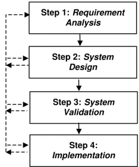
Based on approaches for software development (wa-terfall lifecycle (Whitten, 1995)), for development of discrete event dynamic control system (Miyagi, 1996), and for continuous control system development (Ogata, 1990), the HVAC control system development is divided
Step 2:
System
Design
Step 3:
System
Validation
Step 1:
Requirement
Analysis
Step 4:
Implementation
Figure 4: Steps of HVAC control system development process.
into four main steps (Figure 4):
The Step 1 consists of the identification of the control system purposes, i.e., what the system should do, what are possible interactions with users and what are possi-ble interactions with a high level control system. Local control systems should also be specified by defining the input/output variables of each local controller.
In the Step 2, it should be determined how the con-trol system will perform the activities defined in Step 1. During this phase, the modeling activity has an im-portant role, since it is responsible for guiding designers throughout the design process.
In the Step 3, the models built in Step 2 should be an-alyzed in order to validate the overall system behavior according to the requirements defined in Step 1.
Finally in Step 4, models should be codified in any pro-gramming language and implemented. It is also part of this step the selection of hardware equipment.
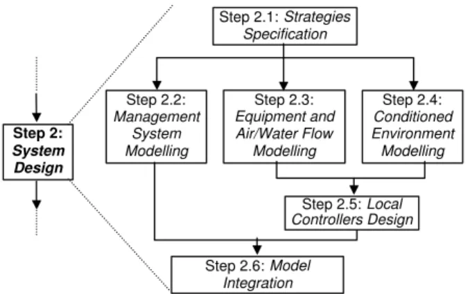
The focus of this paper is on the Step 2. The design phase should embody the modeling of the HVAC control system, the HVAC equipment, the water/air flow, and the environment. For this purpose, a further division of Step 2 is proposed in this paper (Figure 5).
Step 2:
System Design
Step 2.2: Management
System Modelling
Step 2.1: Strategies Specification
Step 2.3: Equipment and Air/Water Flow
Modelling
Step 2.5: Local Controllers Design
Step 2.6: Model Integration
Step 2.4: Conditioned Environment Modelling
Figure 5: Decomposition of Step 2 – System Design.
be defined considering the systems requirements of Step 1. It should also consider how the HVAC Management System could improve the local controller performance based on events treated by the Building Management System or based on the thresholds informed by the local processors. The models of the HVAC Management Sys-tem, equipment, air/water flow and conditioned envi-ronment should then be built. According to these mod-els local controllers should be designed by defining the controller configurations and its constants. Finally, in Step 2.6 all the models should be integrated into a global model of the HVAC system (including control system and controlled object).
Each step is presented with more detail in the following, using as example the models developed for the HVAC system of an ambulatory building.
3.2
The Example
The proposed approach is applied to the HVAC sys-tem of the Ambulatory Building of the Medical School Hospital of University of S˜ao Paulo. Giving an idea of its complexity, the ambulatory is a building of about 100,000 m2
, which includes clinics, surgery center and industrial pharmacy, among other installations. The In-telligent Building concept cannot be fully implemented at the ambulatory building, but its HVAC system can be used as a reference model. The ambulatory HVAC system includes heating and cooling. The chilled water is centrally produced by 8 chillers and 8 cooling towers. The hot water is produced by 2 boilers. The water is then distributed to various coils. Each coil conditions a zone. A zone is a conditioned environment under the control of a single temperature sensor. The Ambula-tory Building is divided into 370 zones. In this paper a simplified version of the modeling of one of its zone is
PI
Mixing box
HVAC Zone System
Supply fan
Air from zone
Cooling coil Air from
outside Air to outside
Air to zone
Signal from zone temperature
sensor Return fan
Three-way valve
Figure 6: HVAC zone system.
presented as an example. The complete models of the HVAC system, including the hot and cool water produc-tion, can be found in [Villani, 2000].
A scheme of the HVAC zone system adopted as an ex-ample is presented in Figure 6. Basically, the zone tem-perature is controlled by changing the amount of water that passes through the cooling coil. A three-way valve controls the water flow in the heating/cooling coil. The airflow is maintained by two fan. In the zone the mixing-box performs the partial or complete air renovation. In the following section, each step of the proposed approach is detailed for this zone system.
3.3
Step 2.1: Strategy specification
Strategies of the HVAC Management Systems are com-posed by discrete event sequences that are executed un-der certain conditions. These events are commands sent to local controllers and equipment in order to change their configurations. The strategy specification is an in-termediate step after the requirement analysis and be-fore the system modeling. It consists of a textual de-scription and uses no formalism. The dede-scription must contain the event sequence of each strategy and the con-ditions under which the strategy is performed.
For the ambulatory zone example the following strate-gies are considered:
Fire Strategy: it is activated and maintained when fire is detected in the zone. The event sequence is:
• the mixing box is set to take 100% of outside air;
even-tual unbalance of the system due to the great de-mand of cold water;
• the return fan speed is increased to prevent smoke diffusion and the supply fan is turned on.
Unoccupied Zone Strategy: it is activated and main-tained when there is nobody in the zone and fire is not detected, or when there is an order by the BMS or the user and fire is not detected. The event sequence is:
• PI valve controllers are turned off;
• fans are turned off;
• simultaneously to the fans setting, the mixing box is set to take 0% of outside air
Occupied Zone Strategy: it is activated and main-tained when there is someone in the zone and fire is not detected or when there is an order by the BMS or the user and fire is not detected. The event sequence is:
• the mixing box is set to take 60% of outside air;
• simultaneously to the mixing box setting, fans are turned on;
• PI valve controllers are turned on;
• PI valve controller switches configuration according to the occurrence of discrete events that change the thermal load in the zone.
The PI valve controller switching activity of the Occu-pied Zone Strategy is introduced to reduce the HVAC time lag between the occurrence of a disturbance (dis-crete thermal load variation) and its compensation by the HVAC control system. Briefly, the reason for the time lag in the HVAC response is the large thermal inertia of the whole system (Honeywell, 1995). How-ever, this time lag could be reduced if a modification in the thermal load instantly causes a modification in the HVAC control system. By switching PI configurations according to the occurrence of discrete events that cause thermal load variation detected by other building sys-tems, the duration and amplitude of these disturbances can be reduced while improving users thermal comfort.
3.4
Step 2.2: Management System
Mod-eling
Starting from the textual description of the manage-ment strategies, a top-down method based on Petri net
Arc Activity
Activity 1 Inter-activity
Activity 2
Activity 3
Figure 7: PFS components.
Activity 1
c) a)
Activity 1
Activity 1a Activity 1b
b)
Activity 1
Activity 1a
Figure 8: Production Flow Schema refinement sequence.
and Production Flow Schema is applied to build sys-tem models. Firstly, a conceptual model is obtained by using the Production Flow Schema modeling technique (Miyagi et al, 1997). Then, the Production Flow Schema is refined into a functional model using P/T Petri nets.
The Production Flow Schema is derived from inter-preted graphs (channel/agency net) (Reisig, 1985) and, essentially, describes the activities performed in a flow of discrete items in a high level of abstraction. Production Flow Schemas have no dynamic. Its components are activities, which represent modifications on the flow of items, inter-activities, which are passive elements, and arcs (Figure 7).
Each activity of a Production Flow Schema is detailed
into a new Production Flow Schema (Figure 8a), a Petri Net model (Figure 8c), or a mixed Production Flow Schema/Petri Net model (Figure 8b). During the re-finement process,activities should be replaced by mod-els beginning and ending with either an activity or a Petri nettransition, in order to guarantee the coherence of the resulting Petri Nets.
Based on the Production Flow Schema/Petri net refine-ment procedure, the HVAC Managerefine-ment modeling is decomposed into the following steps:
Execute Unoccupied Zone Strategy Execute Occupied Zone Strategy
Execute Fire Strategy
Figure 9: Production Flow Schema of Step 2.1.1.
built showing the relation between the strategies, i.e., if they are concurrent, complementary, can be executed at the same time, etc. In this Produc-tion Flow Schema each strategy is modeled as an activity.
Step 2.2.2- Each strategy of the previous Production Flow Schema is detailed according to its sequence of events.
Step 2.2.3- The communication with the Building Management System and the User Interface (which enable or disable strategies) is performed by en-abling and inhibitor arcs (Silva & Miyagi, 1996). In this case the control signal carried by thearcs is a logical combination of the information from the Building Management System. According to their value the arcs inhibit or enable the beginning or end of anactivity.
Step 2.2.4- Each activity of the strategy is detailed into a P/T Petri net model. At this level, the
ac-tivity is modeled as a command that is sent to the
correspondent equipment or local control system. Before passing to the nextactivity, the supervisory system must receive an acknowledge of the com-mand execution.
Step 2.2.5- The communication between the Petri net strategy model and the equipment or local control system models is also performed by addingenabling arcs.
In the following, these steps are applied to the ambu-latory zone example. Figure 9 presents the Production Flow Schema of Step 2.1.1. According to the textual description of the strategies, they are all concurrent.
By Step 2.1.2, this model is detailed into the Produc-tion Flow Schema of Figure 10. Then theenabling and
inhibitor arcs integrate the HVAC Management System
with Building Management System and User Interface
Control signal 2 Move mixing box to
60% of outside air
Switch controller to next configuration Switch controller to previous configuration Turn on PI
valve controller
Control signal 1 Control
signal 1
Control signal 3
Execute Occupied Zone Strategy
Turn on return fan
Turn on supply fan
Enabling arc
Inhibitor arc
Figure 10: Detailed Production Flow Schema (Step 2.1.2).
(Step 2.1.3), according to the textual description of the strategies.
The control signals are calculated according to the fol-lowing expressions:
Control signal 1: NOT(F)AND (BOR UOR P)
Control signal 2: (NP old – NP new)*CP + (NL old – NL new)*CL + (NE old – NE new)*CE>Qmin
Control signal 3: (NP new – NP old)*CP+ (NL new – NL old)*CL + (NE new – NE old)*CE>Qmin
where :
• F is the signal from the Building Management Sys-tem indicating fire in the zone (this information is given by fire system);
• B is the signal from the Building Management Sys-tem imposing this strategy;
• U is the signal from the User Interface imposing this strategy;
• P is the signal from the Building Management Sys-tem indicating that there are people in the zone (this information is given by the access control sys-tem);
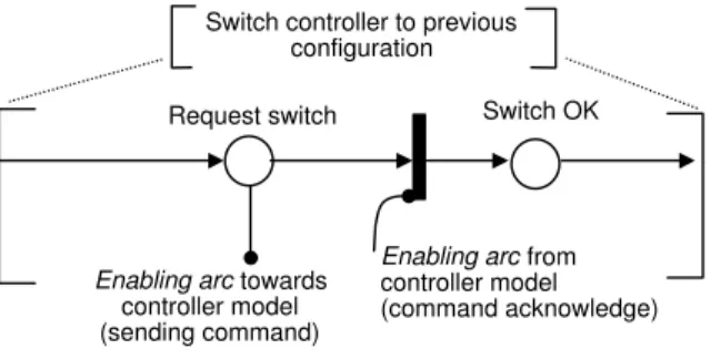
Switch controller to previous configuration
Request switch
Enabling arc from controller model (command acknowledge) Enabling arc towards
controller model (sending command)
Switch OK
Figure 11: Petri net model of anactivity
• NP new is the is the information from the Building Management System about the number of people in the zone now (this information is given by the access control system);
• CP is a constant associated with the thermal load of one person;
• NE old, NE new, CE, NL old, NL new, CL – idem of NP old, NP new, CP for equipment and lights.
• Qmin is a constant associated with the minimal thermal load variation for switch controller config-uration.
Subsequently, the model of Figure 10 is refined into a Petri net model (Figure 11), according to Step 2.1.4 and 2.1.5.
3.5
Step 2.3:
Equipment and water/air
flow modeling
At this step, a hybrid approach is necessary to model both equipment discrete states and water/air continu-ous variables. The Production Flow Schema has been initially defined for discrete systems, and here an exten-sion of it is introduced for hybrid system modeling. In this case, the refinement of eachactivity uses the DPT Petri net [Champagnat, 1998] and differential equation systems. In the DPT Petri net model the link between
the activities is made by the continuous variables,
in-stead oftoken flows as in Step 2.2.
The procedure for building the Production Flow Schema for hybrid systems is divided in the following steps:
Step 2.3.1- The relevant fluid properties should be chosen. Basically, these properties are those that are necessary for evaluating the system perfor-mance, that are the inputs and outputs of the local
Air in the mixing
box
Imposing air flow on supply
fan
Cooling air on coil
Air from
outside Air towards outside Air
from
zone Air to zone
T2_in f2_in
Flow division on
valve
Water flow mixture T6_in
f6_in T6_out f6_out T2_out
f2_out T3_in
f3_in T3_out
f3_out T4_in
f4_in T4_out f4_out
T5_in f5_in
Vector of variables
Imposing air flow on return
fan T1_in
f1_in T1_out
f1_out
Chilled water
Chilled water
Figure 12: PFS model of air and water flow through zone equipment.
control system, and all the others that are necessary to calculate the previous ones.
Step 2.3.2- The Production Flow Schema is built by determining the sequences of activities performed on the fluid. Anactivity is any modification on the relevant properties along the process.
Step 2.3.3- For each activity, a vector of variables is defined for the beginning and the end of theactivity, representing fluid properties at that point of the process
Figure 12 illustrates the Production Flow Schema built for the ambulatory zone example. In this case, there are two fluids: water and air. The relevant properties are flow (f) and temperature (T).
The refinement procedure of the Production Flow Schema for hybrid systems is divided in the following steps:
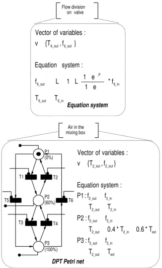
Step 2.3.4- Each activity of the Production Flow Schema can be detailed into a new Production Flow Schema, a DPT Petri net and/or an equation sys-tem. The equation system is used to determine the relation between the properties at the begin-ning and at the end of an activity. The DPT Petri net is used in the case that the equipment perform-ing theactivity can assume different discrete. Each state of the equipment is represented by a place, which is associated to an equation system.
6_in 6_out 6_in P . 6_out 6_out 6_out T T f * e 1 e 1 L 1 L f : system Equation } f , {T v : variables of Vector ext 2_out 3_in 2_out ext 2_in 2_out 3_in 2_out 2_in 2_out 3_in 2_out 2_out 2_out T T f f : P3 T * 6 . 0 T * 4 . 0 T f f : P2 T T f f : P1 : system Equation } f , {T v : variables of Vector Flow division on valve
Air in the mixing box P1 (0%) P2 (60%) P3 (100%) T1 T2 T4 T3 T6 T5 Equation system
DPT Petri net
Figure 13: Detailed model foractivity[Flow division on valve] and [air in the mixing box].
Step 2.3.6- Inter-activities represent system parts where no modification is performed on fluid proper-ties. However, properties in the end of an activity are not the same of the beginning of next activity because the air that is leaving an activity“spends some time” to arrive in the beginning of the next activity. In order to represent this time delay, equa-tion systems are associated with inter-activities.
As an example, Figure 13 shows the activity [Flow di-vision on valve] detailed into an equation system, and theactivity[Air in the mixing box] detailed into a DPT Petri net.
In Figure 13 the following notation is used in the equa-tion systems:
• P is the position of the three-way valve;
T 2_in 1_out 2_in f 2_in 1_out 2_in
T
T
dt
dT
f
f
dt
df
T1_outf1_out T2_inf2_in
Figure 14: Example of inter-activity refinement.
• β,L are valve constants;
• P1, P2, P3 represent the mixing box position of 0%, 60% and 100% of airflow renovation.
As an example, the equation system for the first inter-activity is presented Figure 14.
3.6
Step 2.4:
Conditioned environment
modeling
The model of the conditioned environment is also com-posed by differential equations and DPT Petri nets. The following steps are defined for the conditioned environ-ment modeling:
Step 2.4.1- An equation system determines the evolu-tion of the relevant properties of the zone according to the properties of the airflow entering in the zone and external variables.
Step 2.4.2- Discrete events that may influence the dy-namic of the zone properties are modeled by DPT Petri nets.
For the example of the ambulatory zone, the equation of Step 2.4.1 must determine the air temperature within the zone according to the incoming flow of the HVAC system, thermal loads introduced across walls and by equipment, people and lights. In this case, the thermal load can be modified by discrete events (light is turned on, someone enters in the zone) and is modeled using DPT nets. The zone equation system and the DPT Petri net associated to the people thermal load are presented in Figure 15.
In Figure 15 the following notation is used in the equa-tion systems:
p air HVAC light people zone c * * vol ... Q Q Q T
K
Q
Q
:
T1
of
Fuction
Junction
}
Q
{
v
:
variables
of
Vector
people people people People enter inthe zone
T1
Differential equation system
DPT Petri net
Conection by continuous variable
Qpeople
P1
Figure 15: Zone model.
• K is the thermal load of a person, which is consid-ered constant.
• Tzone, volair are the temperature and the volume of air in the zone;
• ρ,cpare the air density and the specific heat at con-stant pressure;
3.7
Step 2.5: Local Control System Design
Possible configurations of local controllers must be spec-ified considering the interactions with the supervisory system defined previously. The fixed parameters for each controller configuration must be designed together with a switching configuration policy. Each local control system is then modeled by a DPT Petri net.
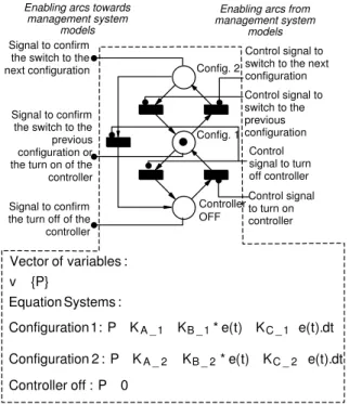
In the ambulatory zone example, two configurations are considered for the PI controller of valve position. They are switched according to the signal from the manage-ment system. The DPT Petri net is presented in Figure 16. This model is connected to the management sys-tem model of Figure 11 by the enablingarcs, and to the equation system model of Figure 13 by the continuous variable P.
In Figure 16 the following notation is used in the equa-tion systems:
• P is the position of the three-way valve;
0 P : off Controller dt ). t ( e K ) t ( e * K K P : 2 ion Configurat dt ). t ( e K ) t ( e * K K P : 1 ion Configurat : Systems Equation {P} v : variables of Vector 2 _ C 2 _ B 2 _ A 1 _ C 1 _ B 1 _ A Signal to confirm
the switch to the previous configuration or the turn on of the controller Config. 2 Config. 1 Controller OFF Control signal to turn off controller Control signal to switch to the next configuration Control signal to switch to the previous configuration
Control signal to turn on controller Enabling arcs towards
management system models
Enabling arcs from management system
models Signal to confirm
the switch to the next configuration
Signal to confirm the turn off of the controller
Figure 16: Local control system model.
• e(t) is the difference between zone temperature (continuous variable of zone model of Stage 3) and its setpoint;
• β,L are valve constants;
• K1A, K2A, K3A, K1B, K2B, K3B are controller
constants at each configuration.
3.8
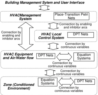
Step 2.6: Model integration
Building Management Sytem and User Interf ace
Connection by enabling and inhibitor arcs
HVACManagement System
Place-Transition Petri Nets
HVAC Local Control System
HVAC Equipment and Air/Water flow
Zone (Conditioned Environment)
DPT Nets Equation
Systems Connection by
continuous variables
DPT Nets
Connection by continuous variables
Connection by continuous variables
Equation Systems
DPT Nets
Connection by continuous variables Connection by enabling
and inhibitor arcs
Figure 17: The resulting model structure.
4
CONSIDERATIONS ABOUT THE
SYS-TEM VALIDATION
Once that the model of the HVAC control system is built, the next step, according to Figure 4, is Step 3 – System Validation. This step can include model sim-ulation and the verification of formal properties of the model.
The model simulation can be used to analyze the sys-tem behavior under certain conditions. An example would be verifying if the PI controllers meet theirs re-quirements in extreme situations, such as with the most abrupt thermal load variation. Another example can be to calculate the average energy consumption. In this case, some transition could be turned into stochastic timed transition (as in Stochastic Petri nets). As an example, the entering of people in the zone (transition T1 of Figure 15) could be associated to distributions representing day/night occupation of the building. To each situation, it is possible to determine the number of chillers and fans that are on at each time, and therefore, average energy consumption.
For model simulation, two kinds of simulators should be accomplished: one of Petri nets and one of differential equations. Simulators must be synchronized by events. Figure 18 illustrates the steps for a hybrid system sim-ulation.
Firstly, the initial state is defined (the initial mark-ing and initial values of continuous variables). Then, it is verified if any transition is active and could be
Definition of initial marking and initial variable values
Fire a transition.
Time increment.
NO YES
Could any transition be fired?
Solve equations.
Figure 18: Hybrid system simulation.
fired. Both P/T net transitions and DPT net
transi-tions should be tested. If possible, active transitions
are fired. When no moretransitioncould be fired, a nu-meric simulation using the current system of equations is performed. Between every increment of simulation time a test must be performed to verify if anytransition could be fired. The simulation data is then used in per-formance analysis methods such as the PMV (people average vote) and PPD (percentage of people unsatis-fied) [Fanger, 1970].
In order to analyze the ambulatory HVAC sys-tem, a simulator has been developed using MAT-LAB/SIMULINK?. Basically, the differential equation systems of the DPT Petri net are simulated by block diagrams in Simulink. The P/T Petri net model and the discrete part of the DPT Petri net model are sim-ulated by MatLab subroutines and incorporated in the Simulink model by the theMatLab-Fuction block. The interface between the two parts (the enabling and junc-tion funcjunc-tions and the choice of the equajunc-tion system) are also established by Simulink blocks. The synchroniza-tion between the two parts is guarantee by the Simulink clock. More details about the developed tool can be found in [Villani et al, 2002 (a)]
a)
b)
8 9 10 11 12 13 14 15 16 17 18 -2
0 2 4 6 8 10 12 14
0.5 1 1.5 2 2.5
time (hours) without integration
with integration
event occurrenc
e
event occurrenc
e
0 21. 5
22 22. 5
23 23. 5
24 24. 5
Room temperature (ºC)
Economy of cold water (%)
time (hours) people arrive in the room
people leave in the room
Figure 19: Examples of simulation results.
thermal comfort can be estimated. The second example compares the cold water consumption with or without the use of the “Unoccupied Zone Strategy”. It is sup-posed that the zone is not used during between 10:00 and 12:00 in the morning and between 14:00 and 16:00 in the afternoon. Figure 19 b) presents the percentage of economy of cold water during the day.
The other way of validating the system is by verifying formal properties of the model. In this case, the prop-erty may concern only the discrete part of the model or both the continuous and discrete part.
In the first case, all approaches developed for verifying the Petri net properties could then be used for the sys-tem behavior analysis, such as invariants, reachability,
liveness, boundedness, etc. As an example, it is possi-ble to guarantee that not more than one strategy is on at a time by verifying if it is 1-boundedness. It is also possible to guarantee that one, and only one strategy is on by verifying if the management system Petri net is a place invariant. By building the reachability tree it is possible to guarantee that a situation not allowed will never happen, such as the PI controller is ‘ON’ and the fans are ‘OFF’.
When verifying properties that involve the continuous and discrete aspects of the hybrid model, a major prob-lem arises: the non-decidability. This means that there is no guarantee that the property can be proved with a finite number of steps. As it has been proven by (Alur et al, 1995), if continuous variables with different growing rates (different derivatives) are included in the model, then the reachability may become undecidable.
Generally, this is the case of the HVAC system models. Even with no guarantee of a solution, many methods are being studied for proving properties of hybrid systems. In [Silva et al, 2001] a comparative study of the state of art in algorithmic approaches for the verification of hy-brid system is presented. According to it the complexity of the computation restricts the application of the ap-proaches for fairly small systems (systems with around 5 continuous variables and non-linear dynamic can re-quire some hours of computation and enormous memory consumption). This problem is mainly due to the fact that these approaches are based on model checking, i.e., they must cover all the possible state-space in order to verify a property.
[Villani et al, 2002 (b)].
5
CONCLUSIONS
In this paper, a novel hybrid modeling approach for HVAC control system design in Intelligent Buildings has been introduced. The hybrid approach is necessary in order to achieve system integration. This top-down approach starts from Production Flow Schema models, and by successive refinements Petri net models are built considering system integration with other building sys-tems. The discrete part is modeled using P/T Petri nets and the continuous part is modeled using differen-tial equation systems. The interface between these two parts is provided by DPT nets. Although other tools might be used, Petri net is chosen due to its graphical capacity of representing concurrency, parallelism and se-quencing of events, which are more suitable with the level of abstraction of the HVAC Management System.
The problem of HVAC control system behavior analysis is also approached. For the discrete part, the formal analysis techniques of Petri nets could be used. For the overall hybrid system simulation, a simulator has been developed using MATLAB/SIMULINKr. Methods for the formal verification of model properties are also under development.
Once the models have been analyzed, it should be trans-lated into a programming language code in order to be implemented. Future directions of this work must also contemplate a method for translation that guaran-tee that the behavior modeled and analyzed using Petri nets will be preserved.
ACKNOWLEDGEMENTS
Authors acknowledge the collaboration and financial support of the Medical School Hospital of the Uni-versity of S˜ao Paulo (HC-FMUSP), and the Brazilian governmental agencies FAPESP, CNPq, CAPES, RE-COPE/FINEP. They also thank Prof. Emilio C. N. Silva for the English language revision.
REFERENCES
Alla, H. & David, R. (1998). Continuous and Hybrid Petri Nets,Journal of Circuits, Systems and Com-puters, Vol.8, n.1, pp. 159-188.
Antsaklis, P. J. & Nerode, A. (1998). Hybrid Control
Systems: An Introductory Discussion to the Spe-cial Issue. IEEE Transactions on Automatic Con-trol, Vol.43, pp. 457-460.
Arkin, H. & Paciuk, M. (1995) Service Systems Integra-tion in Intelligent Buildings. Proc. of IB/IC Intel-ligent Buildings Congress, Telaviv.
Becker, R. (1995). What is an Intelligent Building.Proc of IB/IC Intelligent Buildings Congress, Telaviv.
Champagnat, R. et al (1998). Modelling and Simulation of a Hybrid System through Pr/Tr PN-DAE Model.
Proc.of the 3th International Conference on
Au-tomation of Mixed Processes (ADPM’ 98),Reims.
David, R & Alla, H. (1994). Petri Nets for Modeling of Dynamic Systems – A Survey.Autom´atica, Vol.30, n.2, pp.175-201.
Fanger, P.O. (1970). Thermal Comfort, McGraw-Hill, New York.
Gu´eguen, H. & Lefebvre, M. A. (2000). A comparison of mixed specification formalisms. Proc.of the 4th International Conference on Automation of Mixed
Processes (ADPM 2000), Dortmund.
Ho, Y.C. (1989). Scanning the issue - Dynamics of dis-crete event systems. Proceedings of IEEE, Vol.77, pp. 3-6.
Honeywell (1995). Engineering Manual of Automatic
Control – HVAC. Honeywell, New York.
Miyagi, P. E. (1996).Controle Program´avel -
Fundamen-tos do Controle de Sistemas a EvenFundamen-tos DiscreFundamen-tos,
Edgar Bl¨ucher, S˜ao Paulo.
Miyagi, P.E. et al. (1997). Application of PFS Model Based Analysis of Manufacturing Systems for Per-formance Assessment.Journal of the Brazilian So-ciety of Mechanical Sciences, Vol.19, n.1, pp.58-71.
Ogata, K. (1990) Modern Control Engineering, Engle-wood Cliffs, New Jersey.
Reisig, W. (1985).Petri Nets – An Introduction.Spring Verlag, New York.
Silva, B. I. et al (2001). An Assessment of the Current Status of Algorithmic Approaches to the Verifica-tion of Hybrid Systems. 40th IEEE Conference on
Decision and Control, Orlando.
Villani, E. (2000).Abordagem H´ıbrida para Modelagem de Sistemas de Ar Condicionado em Edif´ıcios In-teligente. Disserta¸c˜ao de mestrado, Escola Polit´ec-nica da USP, S˜ao Paulo.
Villani, E. et al (2002a) Simula¸c˜ao de Sistemas H´ıbridos usando MatLab/Simulink. Anais do II Congresso
Nacional de Engenharia Mecˆanica (CONEM 2002),
Jo˜ao Pessoa.
Villani, E. et al (2000b). Petri nets and Object-Oriented Approach for the Analysis of Hybrid Systems. Anais do XIV Congresso Brasileiro de Automatica
(CBA 2002), Natal.
Whitten, N. (1995). Managing software development