Synchronization of Spatially Extended Chaotic Systems
with Asymmetric Coupling
S. Boccaletti
1, C. Mendoza
1, and J. Bragard
2 1Istituto Nazionale di Ottica Applicata,Largo E. Fermi, 6, I-50125 Florence, Italy
2Departamento de F´ısica y Matem´atica Aplicada,
Universidad de Navarra, E31080 Pamplona, Spain
Received on 18 January, 2005
In this paper, we report the consequences induced by the presence of asymmetries in the coupling scheme on the synchronization process of a pair of one-dimensional complex fields obeying Complex Ginzburg Landau equations. While synchronization always occurs for large enough coupling strengths, asymmetries have the effect of modifying synchronization thresholds and play a crucial role in selecting the statistical and dynamical properties of the highly coupled synchronized motion. Possible consequences of such asymmetry induced effects in biological and natural systems are discussed.
1
Introduction
The synchronization of coupled chaotic systems has been a topic of intense study since 1990 [1]. Interest has now moved to the study of synchronization phenomena in space-extended systems, such as large populations of coupled chaotic units and neural networks [2-4], globally or lo-cally coupled map lattices [5, 6], coupled map networks [7] as well as other space-extended systems [8-13]. Most of the studies have considered synchronization due to exter-nal forcings, or to bidirectioexter-nal symmetric or to unidirec-tional master-slave coupling configurations. In many prac-tical situations, however, one cannot expect to have purely unidirectional, nor perfectly symmetrical coupling configu-rations. As a result, recent interest has focused on detecting asymmetric coupling configurations [14], and quantifying asymmetries in the coupling scheme in relevant applications (such as the study of the human cardiorespiratory system) [15], and then to characterize the effects of asymmetric cou-pling on synchronization (for example between pairs of one-dimensional space extended chaotic oscillators [16]). In par-ticular, Ref. [16] has shown that asymmetry in the coupling of two one-dimensional fields obeying Complex Ginzburg-Landau Equations (CGLE) enhances complete synchroniza-tion, and plays an important role in controlling the properties of the final synchronized state.
This paper presents an account of the synchronization of a pair of non identical CGLE with an asymmetric cou-pling, for both small and large parameter mismatches. We will analyze the type of synchronized dynamics occurring in the presence of asymmetric coupling in all possible dynam-ical states emerging from CGLE, and we will show that in all cases the threshold for the appearance of synchronized motion depends non trivially on the asymmetry in the
cou-pling. We will demonstrate that the selection of the dynam-ics within the final synchronized manifold is always cru-cially affected by the asymmetry. The process leading to synchronization is anticipated by defect-defect synchroniza-tion, inducing the simultaneous appearance in the coupled fields of phase singularities, even in the cases in which the uncoupled dynamics of both fieldsdoes notinclude the pres-ence of defects.
2
Model equation for synchronization
We will consider a pair of one-dimensional fields obeying Complex Ginzburg-Landau Equations (CGLE). This equa-tion has been extensively investigated in the context of space-time chaos, since it describes the universal dynami-cal features of an extended system close to a Hopf bifurca-tion [17], and therefore it can be considered as a good model equation in many different physical situations, such as occur in laser physics [18], fluid dynamics [19], chemical turbu-lence [20], bluff body wakes [21], or arrays of Josephson’s junctions [22].
We will consider a pair of complex fieldsA1,2(x, t) =
ρ1,2(x, t)eiφ1,2(x,t) of amplitudes ρ
1,2(x, t) and phases
φ1,2(x, t), whose dynamics obeys
˙
A1,2=A1,2+(1+iα)∂x2A1,2−(1 +iβ1,2)|A1,2|2A1,2 + c2 (1∓θ)(A2,1−A1,2).
(1) Here, dots denote temporal derivatives,∂2xstays for the second derivative with respect to the space variable0≤x≤
a parameter accounting the for asymmetry in the coupling. The caseθ = 0describes the bidirectional symmetric cou-pling configuration, whereas the caseθ = 1(θ = −1) re-covers the unidirectional master slave scheme, with the field
A1(A2) driving the response ofA2(A1).
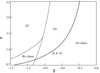
Whenc = 0(the uncoupled case), different dynamical regimes occur in Eqs. (1) for different choices of the para-metersα, β [23-25]. The full parameter space for the dy-namics of the CGLE is shown in Fig. 1. In particular, Eqs. (1) admits plane wave solutions (PWS) of the form
Aq(x, t) =
p
1−q2ei(qx+ωt) −1≤q≤1. (2) Here,qis the wavenumber in Fourier space, and the tem-poral frequency is given by ω = −β −(α−β)q2. The stability of such PWS can be analytically studied below the Benjamin-Feir-Newel (BFN) line (defined byαβ = −1 in the parameter space). Namely, forαβ >−1, one can define a critical wavenumber
qc=
q
1+αβ
2(1+β2)+1+αβ (3) such that all PWS are linearly stable in the range −qc ≤
q≤qc. Outside this range, PWS become unstable through
the Eckhaus instability [26].
AT
PT
B−F−N
α
−0.6
−1.5 −1.2 −0.9 −0.3 0.0
0.7 1.4 2.1 3.5
2.8
No chaos
β
Bi−chaos
Figure 1. (α,β) parameter space for Eqs. (1) forc= 0. The lines delimit the borders for each one of the dynamical regimes produced by Eqs. (1), and the Benjamin-Feir-Newel line for stability of the plane wave solutions.
When crossing from below the BFN line in the para-meter space, Eq. (3) shows that qc vanishes and all PWS
become unstable. Above this line, Refs. [23-25] identify different turbulent regimes, called respectively Amplitude Turbulence (AT) or Defect Turbulence, Phase Turbulence (PT), Bi-chaos, and a Spatiotemporal Intermittent regime. The borders in parameter space for each one of these dy-namical regimes are schematically drawn in Fig. 1, together with the BFN line. In this work, we will mainly concentrate on PT and AT, since they constitute the fundamental dynam-ical states for the evolution of the uncoupled fields, and their main properties [27] have received considerable attention in
recent years including the definition of suitable order para-meters marking the transition between them [28], as well as for the study of synchronization in bidirectional symmetri-cal coupling configurations [11,29-31].
PT is a regime where the chaotic behavior of the field is mainly dominated by the dynamics of φ(x, t), the am-plitudeρ(x, t) changing only smoothly, and being always bounded away from zero. On the other hand, AT is the dynamical regime wherein the fluctuations of ρ(x, t) be-come dominant over the phase dynamics. Here, the complex field experiences large amplitude oscillations which can (lo-cally and occasionally) causeρ(x, t)to vanish. As a con-sequence, at all those points (hereinafter called space-time defects or phase singularities) the global phase of the field Φ≡arctanhImRe((AA))
i
shows a singularity.
3
Characterization of synchronized
states
The purpose of our paper is to report the different synchro-nization states that are selected when an asymmetric cou-pling takes place between the two CGLE fields. In order to be as exhaustive as possible, we will consider different regimes for the two CGLE. The reference as a starting point is the case treated in Ref. [16] (i.e. α = 2,β1 = −0.7 andβ2 =−1.05). For this parameter choice, the two fields are originally prepared to display PT and AT, respectively. As a consequence, hereinafter we will denote this situation as PT-AT(I). Another possible choice for an initial PT-AT configuration, whose relevance will be momentarily clear, is to considerα= 2,β1=−0.95andβ2=−1.2(we will denote such a situation as PT-AT(II)). Finally, we will con-sider also cases of small parameter mismatch, where the two systems start from the same initial dynamical state, such as
α= 2,β1=−0.75andβ2=−0.9(denoted by PT-PT) and
α= 2,β1=−1.05andβ2=−1.2(denoted by AT-AT).
-1.2 -1 -0.8 -0.6
0.7 0.8 0.9 1
ω
β
Figure 2. Natural averaged frequencyω(see text for definition)vs.
βforα = 2. The filled dots report the values from simulations of Eqs. (1) atc= 0. The dashed lineω= −βis the prediction
In all cases, we consider values of the asymmetry pa-rameter θ ∈ [−1,+1], and highlight the effects of asym-metry in the synchronization properties (c 6= 0) of system (1). Simulations were performed with a Crank-Nicholson, Adams-Bashforth scheme (which is second order in space and time [32]), with a time stepδt= 10−2
and a grid size
δx= 0.25, forL= 100(corresponding to 400 grid points) and spatial periodic boundary conditions [A1,2(0, t) =
A1,2(L, t)].
A crucial parameter in all our investigations, that dic-tated the choice of the parameters in the different cases, is the natural average frequency of the single CGLE. Such a frequency is calculated from the numerical simulations of a single CGLE by averaging in space the unfolded phaseφ
defined inRrather than in[0,2π]. We have:
ω= lim
t→∞
< φ(x, t)>x
t (4)
where< ... >xrepresents for a spatial average.
Figure 2 showsωvs.the parameterβatα= 2. In order to construct Fig. 2, we have integrated the CGLE for a very long time (tf = 15,000) after eliminating transient
behav-iour (T = 5,000). Two different initial conditions for each value of β were chosen in order to measure the sensitivity of ωwith respect to selection of different initial condition. It should be emphasized that all initial conditions were cho-sen to have a zero average phase gradient [28], because the frequency in the PT regime is highly sensitive to the average phase gradient as shown by [28].
From Fig. 2 one clearly realizes thatω reaches a max-imum for β ≈ −0.98, close to the transition from the PT to the AT regime. This transition has been extensively stud-ied by several authors [28, 33, 34], and it has been shown that it depends on the spatial extension on which the Eqs.(1) are integrated, as well as on the average phase gradient. In addition, it is interesting to notice (see Fig. 2) that on the right hand side of the maximum (PT regime) the two differ-ent initial conditions lead to nearly the same value for the averaged frequency, while on the left hand side of the max-imum (AT regime) the two initial conditions lead in general to two different values for ω. This fact could serve as an alternative indicator for the characterization of the PT-AT transition. Furthermore, the frequency difference between the prediction given by the dispersion relation of the PWS (dashed line) and the numerical simulations can be evalu-ated quite accurately in the PT regime (right hand side of the maximum) by using the modified Kuramoto-Sivashinsky equation [35, 36].
Considerations based on Fig. 2 dictate the choice for the parameters β’s in the rest of the presentation. Indeed, a question to be clarified is how crucial is the role of the natural frequency for the selection of the dynamics for the two coupled CGLE in the synchronized state. A previous study with bidirectional symmetrical coupling configuration (θ= 0) between a PT and a AT regime [11] pointed out that the final synchronized dynamics occurs in a PT state. The above result was obtained for a parameter choice for which the frequencyωP T of the initial PT state was smaller than
the one (ωAT) of the initial AT state. This was also the
situ-ation of the case PT-AT(I) treated in Ref. [16] (see Fig. 2).
We will show that, in the absence of asymmetries, the dy-namics in the final synchronized state isalwaysselected to correspond to that state having an originally smaller value ofω. This property has dictated the choice of parameters for the case PT-AT(II) considered in the present Manuscript (β1=−0.95andβ2=−1.2). In this case Fig. 2 shows that
ωP T > ωAT, and we will see that the synchronized motion
atθ= 0develops onto a AT regime.
Let us now discuss how to characterize the synchroniza-tion properties of the coupled fields by means of suitable indicators [13]. As we are dealing with extended chaotic fields that may be in defect turbulence, concepts of phase synchronization may be hindered by the presence of phase singularities in such regimes, that make average phases dif-ficult to define properly in AT.
On the other hand, complete synchronization (CS) states can be detected by the use of Pearson’s coefficient defined as
γ=p h(ρ1− hρ1i)(ρ2− hρ2i)i h(ρ1− hρ1i)2i
p
h(ρ2− hρ2i)2i
, (5) wherehidenotes a full space-time average (in order to avoid getting spurious values, we allow in general some transient timeT to elapse before evaluating this coefficient). γ mea-sures the degree of cross correlation between the moduli
ρ1(x, t)andρ2(x, t): Whenγ= 0the two fields are linearly uncorrelated, whileγ = 1marks complete correlation and
γ=−1indicates that the fields are negatively correlated.
−1
0
1
0 0.4
0 0.5 1
θ
c
γ
a)
−1 −0.5 0 0.5 1
θ 0
0.2 0.4 0.6 0.8 1
γ b)
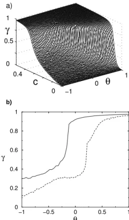
Figure 3. a) Pearson’s coefficientγ(see text for definition)vs.the parameter space(c, θ). Other parameters areα= 2,β1=−0.95
andβ2 =−1.2(case PT-AT(II)). b) Solid line:γvs.θ[cut of the
Another indicator characterizing the disorder in the sys-tem is the number of phase singularities (or defects)N. The-oretically, a defect is a point (x, t) for which ρ(x, t) = 0. This implies that defects are intersections of the 0-level curves in the(x, t)plane of the real and imaginary parts of
A1,2(x, t). In practice, because of the finite size of the mesh and of the finite resolution of the numerics, we must intro-duce a method for the detection of a defect. A reliable cri-terium is to count as defects at timetthose pointsxiwhere
theρ(xi, t)is smaller than0.025 and that are furthermore
local minima for the functionρ(x, t).
It is well known [33, 34] thatNis an extensive quantity of both time and space, and therefore it is sometimes conve-nient to refer to the defect densitynD, that is calculated as
the defect numberNper unit time and unit space.
In the following, we will describe the important effects of asymmetries in the coupling of system (1), for different values of the parametersβ1 andβ2, whileα = 2will be hereinafter fixed.
4
Asymmetry
Enhanced
Synchro-nization
A striking effect of asymmetry in the coupling that has al-ready been highlighted in our previous analysis for the case PT-AT (I) [16] is that one can improve dramatically the syn-chronization threshold by selecting a suitable level of asym-metry in the coupling. Conversely, one can also achieve de-synchronization of the two coupled systems by varying the asymmetry level in the coupling scheme.
4.1
Large Parameter Mismatch
By selecting in (1) a sufficiently large parameter mismatch in the equations forA1,2, one can set the uncoupled evolu-tions ofA1 andA2 to be in PT and AT, respectively. By doing that, one still has three possibilities of choosing the parametersβ accordingly to the natural frequencies of the two separate CGLE.
The first case (PT-AT(I)) corresponds to system 1 in the PT regime (β1 = −0.7) with a lower natural frequency than system 2 in the AT regime (β2 = −1.05). The nat-ural frequencies are approximately equal toω1 ≈ 0.7 and
ω2 ≈0.87 > ω1 (see Fig. 2). This situation has been ex-tensively studied in [16] where both complete and frequency synchronization features were discussed and characterized.
The second case (PT-AT(II)) corresponds to preparing system 1 in the PT regime (β1 =−0.95) with a higher nat-ural frequency than system 2 in the AT regime (β2=−1.2). The natural frequencies are approximately equal toω1≈0.9 andω2 ≈ 0.84 < ω1 (see Fig. 2). For this case, we will show how asymmetry enhances the setting of complete syn-chronization.
Notice that a further situation could be studied where the two systems are prepared in the PT and AT regimes re-spectively, but they have approximatively the same natural frequency. This more complex case, where one might ex-pect some kind of resonance coming into play in the process of synchronization, will be dealt with elsewhere.
Figure 3a reportsγvs.the parameter space(c, θ)for the PT-AT(II) case, and shows the non trivial dependence of the threshold for synchronization on the asymmetry parameter
θ. A better way to visualize such a dependence is by mak-ing a cut of the surface at a fixed value of the couplmak-ing (e.g.
c = 0.25, see Fig. 3b). Both in the PT-AT(II) case and in the PT-AT(I) case (already reported in Fig. 1b of Ref. [16]), a better synchronization level is obtained for the unidirec-tional configuration where the system in the PT regime is driving the system in the AT regime (θ = 1). The surfaces and curves of Fig. 3a;b) have been obtained by making av-erages over a timetf = 15,000after a large transitory has
elapsed (T = 6,000) in order to ensure that we are measur-ing stationary synchronization states.
4.2
Small Parameter mismatch
The very same scenario of asymmetry enhanced synchro-nization occurs when we select small parameter mismatches in Eqs.(1), i.e. we set the parameters so as the two uncou-pled fields are both either in PT or AT, thus confirming that this feature generally characterize the emergence of the syn-chronized motion in our system.
4.2.1 AT-AT Case
In this case, we set β1 = −1.05and β2 = −1.2. Both systems now are in the AT regime, with system 1 having a natural frequency higher than the one of system 2.
−1
0
1 0
0.4 0
0.5 1
c
θ
γ
a)-1 -0.5 0 0.5 1
0.4 0.6 0.8 1
θ γ
b)
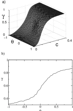
Figure 4. a) Pearson’s coefficientγ(see text for definition)vs.the parameter space(c, θ). Parameters areα= 2,β1 =−1.05and
β2=−1.2(AT-AT case). b)γvs.θ[cut of theγ-surface in a)] at
c= 0.17showing the dependence of the synchronization threshold with asymmetry. Figure obtained by using a statistics over a time
−1 0
1 0
0.5 0
0.5 1
θ
c
γ
a)
-1 -0.5 0 0.5 1
0 0.2 0.4 0.6 0.8 1
θ γ
b)
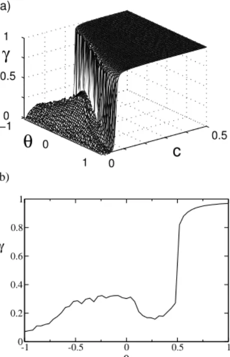
Figure 5. a) Pearson’s coefficientγ(see text for definition)vs.the parameter space(c, θ). Parameters areα = 2,β1 = −0.75and
β2 =−0.9(PT-PT case). b)γvs.θ[cut of theγ-surface in a)] at
c= 0.095. In this case a total timetf = 15,000was using for the calculation of the spatio-temporal averages.
Figs.4 shows Pearson’s coefficient vs. the parameter space(c, θ)(a), as well as a cut of theγ-surface atc= 0.17 (b), showing that asymmetry in the coupling is still playing an important role in modifying the level of synchronization for a fixed value of the coupling strengthc. It is not sur-prising that the complete synchronization threshold is now lower compared to the PT-AT cases. This, indeed, is related to the fact that smaller parameter mismatches induce closer initial dynamics, which are therefore easier to synchronize.
4.2.2 PT-PT Case
Finally, in order to complete this first part of the discus-sion, we examine the PT-PT case. Now, parameters are
β1=−0.75andβ2=−0.9, determining an initial PT state for both uncoupled fields, with system 1 having a lower nat-ural frequency with respect to system 2.
Figures 5a;b describe the behavior ofγas a function of the couplingcand the asymmetryθ. Once again, asymmetry plays a decisive role in enhancing the appearance of a syn-chronized motion in system (1). Notice that here the values ofcrequired for a synchronized motion are smaller than in any of the previous cases, reflecting the fact that the present situation corresponds to the smallest parameter mismatch.
At variance with all the other cases, an interesting fea-ture of Fig. 5b is that an increase in the asymmetry does not always yield a monotonic increase ofγ.
At this stage, we can already draw some interesting con-clusions. We have seen that changing asymmetry in the coupling configuration for the same coupling strength has the effect of enhancing the appearance of a synchronized motion or destroying synchronization, regardless of the ini-tial uncoupled state of the dynamics. We conjecture that this may have relevant consequences in biological systems,
where changes in asymmetry of the interactions could be a way to efficiently synchronize-desynchronize the dynamics for the same strength of interaction.
Furthermore, in Eqs.(1) the coupling is a mapping of all the grid points of system 1 on their corresponding grid points of system 2. We could, in fact, imagine more complicated and probably more realistic configurations where couplings, besides being asymmetric, would be spatially dependent or even asynchronous. While it is likely that real systems show combinations of asymmetric, asynchronous and spatially de-pendent coupling schemes to control and synchronize in an optimal way their dynamical regimes, here we only focused on the effects of asymmetries, since the scenario of emerg-ing dynamics is already extremely rich in this ”simplified” approach.
5
Selection of the Final State
Next, we move to describe how asymmetries play a crucial role in setting the state of the dynamics within the synchro-nized regime, which occur for large values of the coupling strength. Let us recall the methods adopted for our investi-gation of the dynamics within the synchronized regime. Ini-tially (t = 0) we begin a trial simulation of the two Eqs.(1) connected with a non-zero value ofc. We impose random initial conditions on both systems, which in general will have different parameters. As a consequence, the dynamics usually attains synchronized motion only after a transient timeT. Since we are not here interested in characterizing the dynamics in the transient stage, we let a certain transient timeT elapse (we have verified that T = 6,000 is large enough for reaching such asymptotic state) before starting to calculate the indicators of any asymptotic synchronized state. In this way, we can measure such indicators within the statistically stationary state represented by the asymp-totic synchronized motion.
While it is not surprising that when coupling two ini-tially PT states (AT states) the final synchronized motion will persist in the PT regime (AT regime), a relevant point concerns what mechanisms control the selection of the syn-chronized motion, once the two fields originally start from different regimes. To address such an issue, we will focus in the present section on the two PT-AT cases. In these cases, it is not trivial to predicta prioriwhat will be the resulting dynamical state for the synchronized motion.
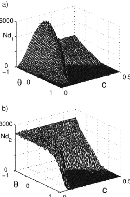
Figures 6a;b show the total number of defects counted for a timetf = 15,000 in the parameter space (c,θ) for
−1 0
1 0
0.5 0
6000
θ
c
Nd
1 a)
−1 0
1 0
0.5 0
3000
θ
c
Nd
2 b)
Figure 6. Total number of defects counted during a timetf = 15,000for the PT-AT(II) case. a) Number of defects appearing in system 1, that was set initially in the PT regime atc= 0; b) Num-ber of defects appearing in system 2, that was set initially in the AT regime atc= 0.
Let us compare and discuss more fully these two cases. In Section (3), we have already seen that the main difference between the cases PT-AT(I) and PT-AT(II) is in terms of the initial natural frequencies of the two subsystems. Namely, in the PT-AT(I) (the PT-AT(II)) case the natural frequency of the subsystem originally set in AT is larger (smaller) than the one of the subsystem originally set in PT. In Fig. 7 we summarize the result of the comparative study of the two cases. We choose a sufficiently large value of the coupling strength so as to ensure a synchronized state, and we have represented with a dashed region (a blank region) the range ofθ-values for which the synchronized motion develops into an AT (a PT) regime.
First of all we observe that at θ = 0(i.e. in the bidi-rectional symmetrical case) the system with a lower natural frequency is the dominant one at the moment of selecting the final synchronized state. Furthermore, in Fig. 7 we ob-serve a very different scenario for the two PT-AT cases. In the PT-AT(I) case a final state in PT is selected for most of the values of the asymmetry parameter (untilθ = −0.84, below which a final state in AT takes over). In contrast, in the PT-AT(II) case for most of the asymmetry values (up to
θ= 0.64) the final state is selected in the AT regime. The conclusion of the present Section is that asymme-tries in the coupling configuration play a decisive role in the selection of the dynamics and the statistical properties of the synchronized state. This feature may have relevant con-sequences in biological and natural systems, where small changes in the asymmetry of the interactions could be used as an efficient way to select the synchronized state of an en-semble of interacting complex units.
−1
−0.5
0
0.5
1
θ
I
II
Figure 7. Dynamical states of the synchronized motion (obtained for large values for the coupling strengthc) attained by the two sub-systems in the PT-AT cases. The upper (lower) bar corresponds to the PT-AT(I) (the PT-AT(II)). The dashed zone refers to a common AT regime while the blank zone marks a common PT regime.
6
Conclusions
In conclusion, we have reported and discussed several asym-metry induced effects in the process of synchronization of a pair of coupled complex space extended fields. While syn-chronization always occurs for large enough values of the coupling strength, the threshold for the setting of synchro-nized motion crucially depends on the asymmetry in the coupling configuration. Furthermore, the asymmetry con-trols in relevant cases the statistical and dynamical prop-erties of the synchronized motion, as is the case when the coupled subsystems start from statistically different dynam-ical regimes. In this latter situation we have shown that a bidirectional symmetrical coupling configuration leads to a synchronized motion where the statistical properties of the subsystem having originally a lower natural frequency pre-vail, whereas asymmetries can drastically change such a sce-nario.
We argue that such features may have relevant con-sequences in biological and natural systems, where small changes in the asymmetry of the interactions could be used as an efficient way to synchronize or desynchronize the dy-namics, as well as select the main statistical properties of the synchronized motion in ensembles of interacting com-plex units.
Acknowledgments
Work partly supported by MCYT project (Spain) n. BFM2002-02011 (INEFLUID).
References
[1] For a comprehensive review on the subject, see: S. Boccaletti, J. Kurths, G. Osipov, D. Valladares, and C. Zhou, Phys. Rep.
366, 1 (2002), and references therein.
[3] A. Pikovsky, M. Rosenblum, and J. Kurths, Europhys. Lett.
34, 165 (1996).
[4] D.L. Valladares, S. Boccaletti, F. Feudel, and J. Kurths, Phys. Rev. E65, 055208 (2002).
[5] V.N. Belykh and E. Mosekilde, Phys. Rev. E54, 3196 (1996).
[6] A. Pikovsky, O. Popovich, and Yu. Maistrenko, Phys. Rev. Lett.87, 044102 (2001).
[7] S. Jalan and R.E. Amritkar, Phys. Rev. Lett. 90, 014101 (2003).
[8] G. Hu and Z. Qu, Phys. Rev. Lett.72, 68 (1994).
[9] L. Kocarev, Z. Tasev, and U. Parlitz, Phys. Rev. Lett.79, 52 (1997).
[10] R.O. Grigoriev, M.C. Cross, and H.G. Schuster, Phys. Rev. Lett.79, 2795 (1997).
[11] S. Boccaletti, J. Bragard, F.T. Arecchi, and H.L. Mancini, Phys. Rev. Lett.83, 536 (1999).
[12] H. Chat´e, A. Pikovsky, and O. Rudzick, Physica D131, 17 (1999).
[13] L. Junge and U. Parlitz, Phys. Rev. E62, 438 (2000).
[14] M.G. Rosenblum and A. Pikovsky, Phys. Rev. E64, 045202 (2001).
[15] M.G. Rosenblum, L. Cimponeriu, A. Bezerianos, A. Patzak, and R. Mrowka, Phys. Rev. E65, 041909 (2002).
[16] J. Bragard, S. Boccaletti, and H. Mancini, Phys. Rev. Lett.
91, 064103 (2003).
[17] For a comprehensive review on pattern dynamics emerging from space-time bifurcations, see: M. Cross and P. Hohen-berg, Rev. Mod. Phys.65, 851 (1993), and reference therein.
[18] P. Coullet, L. Gil, and F. Roca, Opt. Commun.73, 403 (1989).
[19] P. Kolodner, S. Slimani, N. Aubry, and R. Lima, Physica D85, 165 (1995).
[20] Y. Kuramoto and S. Koga, Prog. Theor. Phys. Suppl.66, 1081 (1981).
[21] T. Leweke and M. Provansal, Phys. Rev. Lett. 72, 3174 (1994).
[22] B.D. Josephson, Phys. Lett,1, 251 (1962).
[23] B.I. Shraiman, A. Pumir, W. van Saarlos, P.C. Hohenberg, H. Chat´e, and M. Holen, Physica D57, 241 (1992).
[24] H. Chat´e, Nonlinearity7, 185 (1994).
[25] H. Chat´e, in: Spatiotemporal Patterns in Nonequilibrium Complex Systems, edited by P.E. Cladis and P. Palffy-Muhoray (Addison-Wesley, New York, 1995).
[26] B. Janiaud, A. Pumir, D. Bensimon, V. Croquette, H. Richter, and L. Kramer, Physica D55, 269 (1992).
[27] A. Torcini, H. Frauenkron, and P. Grassberger, Phys. Rev. E55, 5073 (1997).
[28] A. Torcini, Phys. Rev. Lett.77, 1047 (1996).
[29] S. Boccaletti, J. Bragard, and F.T. Arecchi, Phys. Rev. E59, 6574 (1999).
[30] J. Bragard and S. Boccaletti, Phys. Rev. E62, 6346 (2000).
[31] J. Bragard, S. Boccaletti, and F.T. Arecchi, Int. J. of Bifurca-tion and Chaos.11, 2715 (2001).
[32] W.H. Press, et al.,Numerical Recipes in Fortran 90 (Cam-bridge University Press, 1992).
[33] D.A. Egolf and H.S. Greenside, Phys. Rev. Lett.74(10), 1751 (1995).
[34] L. Brusch, M.G. Zimmermann, M. van Hecke, M. B¨ar, and A. Torcini, Phys. Rev. Lett.85, 86 (2000).
[35] H. Sakaguchi, Prog. Theor. Phys.83, 169 (1990).