Leandro de Paula Santos Pereira, Marco Antonio Brasil Terada
Antenna Group, Electrical Engineering Dept., University of Brasilia - DF – [email protected]
Abstract— This article introduces a procedure for determining the optimum design of pyramidal horn antennas. The efficiencies and phase errors in the optimum design are variables and depend on the design requirements. New equations are proposed for the optimum design, which can be solved numerically or analytically.
Index Terms— Antennas, Efficiency, Gain, Optimum Design, Pyramidal Horns.
I. INTRODUCTION
Pyramidal horn antennas are widely used in various applications in the microwave range due to its
high gain, moderate bandwidth and low voltage standing wave ratio VSWR. Its construction is
relativity simple and they are often used as feeders of reflectors and currently in applications where
wide bandwidth is required, such as the technology WiMAX.
The pyramidal horn antenna design consists of determining their dimensions where the gain, the
operation frequency and waveguide to which the antenna will be attached are given. Fig. 1 shows the
antenna and their dimensions. A horn antenna design seeks to determine the values of A, lH or R1, lE or
R2 and B, and these are related by [1]
Fig. 1. Geometry of a pyramidal horn antenna.
2 2 2
1
2 H
A l =R +
(1)
2 2 2
2
2 E
B l =R +
(2)
This work develops a new analytical design technique, using closed formulas based on equations
that take into account the exact phase errors and optimize the gain relative to the E- and H-planes.
Thus, the procedure can be deemed as a consistent, closed form mathematical procedure, which can
be solved numerically and/or analytically with high precision and accuracy.
The usual methods do not consider the exact phase errors and, when they are used, it is assumed
they are constants. Cozzens’s method is based on empirical measurements which give results with a
good accuracy [2], but they do not optimize the antenna gain in relation to the aperture dimensions.
One advantage of the new technique is to provide less variation in the gain with respect to variations
of the aperture dimensions, due to temperature variations for example, if certain conditions of the
directivity curve are satisfied; e.g., if the curve is smooth, which is normally the case with practical
antennas [1]. Thus, the designed antenna can yield a better stability in the gain for the frequency at
which it was designed. Additionally, since the design is based on more accurate equations, the gain
obtained from the design should be closer to reality.
II. ON-AXIS GAIN OF PYRAMIDAL HORN
There are several factors that influence the on-axis gain of pyramidal horns. When calculating the
gain, it is usually assumed that only the dominant mode TE10 is present and propagating within the
antenna; however this does not occur, because when the dimensions of the antenna become larger,
other higher-modes will appear in the antenna aperture, changing its gain [3].
Also, wave reflections are not included in the formulas as it propagates inside the antenna. With the
increase of the aperture, the wave suffers reflections, increasing the value of VSWR. If the transition
from waveguide to free space is made smoothly, there will be fewer reflections and impedance
matching will perform better, resulting in higher operating bandwidth, for example. This occurs when
the flare or aperture angle of the antenna is small and the value of the length of the antenna is large.
Another factor that is not normally taken into account is the oscillation of the gain of pyramidal
with frequency due to multiple diffractions on the aperture edges of the E-plane with further
reflections on the wall of the antenna [4]. These oscillations become increasingly smaller with
increasing of the frequency.
Thus, it can be seen how complex may be the process of determining the gain of the antenna. The
pyramidal antenna gain, ignoring the phenomena discussed above can be given by [1]
2
4
32 E H ap
G D D A B
a b
π λ λ π
ε λ
= =
(3)
with
32
E E
a B
D R
λ π λ
= (4)
32
H H
b A
D R
λ π λ
= (5)
where G is the desired on-axis gain, DE and DH are the gains of the E- and H-planes sectoral horns,
and REand RHare, respectively, the phase error aperture efficiencies in the E- and H-plane, and εap is
2 2 2
( ) ( )
E
C q S q
R
q
+
= (6)
[
]
[
]
{
}
2
2 2
1 2 1 2
( ) ( ) ( ) ( )
64 H
R C p C p S p S p
t
π
= − + − (7)
where C( ) and S( ) functions are Fresnel integrals and
2
q= s (8)
1
1
2 1
8
p t
t
= +
(9)
2
1
2 1
8
p t
t
= − +
(10)
The values of q, p1 and p2 are dependent on the values of phase errors t in the H-plane and s in the
E-plane, given by
2 1
8
A t
R
λ
= (11)
2 2
8
B s
R
λ
= (12)
Equations (3) to (12) were derived by Schelkunoff [5]. These expressions use the geometrical optics
theory and single diffraction at the edges of the aperture antenna. They are used to calculate the
on-axis gain of pyramidal horns and the H-plane sectoral horns [6]. For E-plane sectoral horns, Jull’s
formula for calculating the gain is more accurate [7]. In addition, the maximum possible error
calculated for Schelkunoff’s gain formula using (3) is about ± 0,3 dB [8],[9].
The values of exact phase errors [10] result in a gain close to the measured values, as shown by Fig.
2. They are given by
Fig. 2. Gain curves obtained for a WR284 waveguide with A = 32.41 cm, B = 24 cm, lE= 42.15 cm and lH= 47.45 cm.
−−−analysis using exact phase errors, ⋯⋯analysis using quadratic phase errors, − − − analysis using quadratic phase error in H-plane and Jull’s formula in the E-plane [7], ××× measured values [4],[8].
1/ 2
2 2
2
1
1 16 1 1
8 e
A
t t
t A
λ λ
= + − −
1/2
2 2
2
1
1 16 1 1
8 e
B
s s
s B
λ λ
= + − −
(14)Consequently, to obtain more accurate designs, it is necessary to use (13) and (14) instead of (11)
and (12) in (8) to (10) to calculate the gain and analyzing the results, especially when the antenna
length is small [10]. Jull's formula [7] gives more accurate result when is only used for E-plane
sectoral antennas, because when it is used in the pyramidal antennas, the results are far from the
measured, shown in Fig. 2. The effects of the fringe-currents at the edges on the axis-gain are
different for pyramidal and E-plane sectoral horns, because the last have closely spaced edges
whereas the former have widely spaced edges, which make these effects less significant on the gain of
pyramidal antenna [7],[11].
Usually it is assumed that the optimum aperture efficiency εap in the design is 0.5 or 0.51 [1].
However, this value does not represent the optimum aperture efficiency, but is close to it. In this
work, the optimal design is the result of the choice of the value of A that maximizes the gain in H
-plane for a given axial length R1, and also by choosing the value of B that maximizes the gain in the
E-plane for a given value of R2. It is important to notice that the design is optimum only for the
desired frequency of operation, and does not necessarily also maximizes the aperture efficiency due to
the fact that the gain curve is smooth around its peak.
Commonly the quadratic phase errors are used with t = 0.375 for the H-plane and s = 0.25 for the E
-plane [1]. These values do not optimize the gain or directivity, since these are derived from
approximations of the aperture dimensions that maximize the gain for a given axial length. This
approach lead to
1
3
A≅ λR (15)
2
2
B≅ λR (16)
It is also possible to define the optimum aperture efficiency as 0.49 and optimum phase errors t =
0.4 and s = 0.26 [12].
III. DEVELOPMENT OF AN OPTIMUM DESIGN PROCEDURE WITH A NUMERICAL AND AN ANALYTICAL SOLUTIONS
There are many possibilities to design an antenna, which give several different results in the
dimensions, but produce the same result in the gain. To find a single solution of the design, we have
to obtain a minimum of equations relating the four dimensions that we want to achieve, given the
value of the on-axis gain, the operating frequency and waveguide. The developed procedure uses (13)
and (14) in (3) to (10), and for the antenna to be realizable, the following constrain has to be enforced:
1 2
A a B b
R R
A B
− −
= (17)
For the optimum design, it is chosen A for a fixed value of R1 that maximizes the gain curve in the
dimension A and, through a numerical solution, it is determined the root of this expression, i.e., it is
determined A in function of the independent value R1:
1( , 1)
H
D f A R
A
∂ =
∂
1 1
( ) ( )
A R =root f (18)
where root ( ) is a numerical function that calculates the zeroes of its argument.
The same have to be done to the E-plane, where B is obtained according to the value of R2:
2( , 2)
E
D f B R
B
∂ =
∂
2 2
( ) ( )
B R =root f (19)
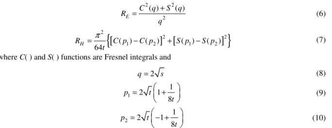
However, these expressions do not have a single root, but many, as can be seen in Fig. 3. Its curve
of directivity has several points where its derivative is zero. This also happens with the directivity of
the H-plane, although the oscillations of the curve are less intense. To select the value of A and B that
maximizes the directivity curve, the root can be chosen so that it is within the range [13]:
Fig. 3. Directivity curve computed with respect to the aperture B with R2=23.65 cm for an operating frequency of 2.5 GHz
using a WR430 waveguide.
1 1
2 2
2
G G
A
λ λ
π < < π
(20)where G is the pyramidal antenna gain. The range of B can be found by the limits of A when using
2
4 ap
G B
A
λ π ε
=
We can estimate εap = 0.49 to find the range of root B, although it is possible to use other values
close to this.
After that, equation (21) is used in order for the dimensions of the antenna to be realizable. As A is
a function of R1 and B is a function of R2, an equation is obtained with two independent variables, R1
and R2. Thus, R1 can be found as the root that satisfies (16) for a given value of R2:
3( 1, 2) 1 2
A a B b
f R R R R
A B
− −
= −
1( 2) ( 3)
Using the previous result in (3), with G being the desired gain value, the numerical solution of the
design is found through the R2 value, since all other dimensions are dependent on R2:
4( 2)
32 E H
f R G D D
a b
π λ λ
= −
2 ( 4)
R =root f (22)
It is possible to develop an analytical method for this design based on the results, where it is
verified that the exact phase errors vary with the requirements of gain, the dimensions of the
waveguide and the operation frequency. When a waveguide with 2 ≤ a/b≤ 2.5 and frequency in the
range 1 < λ/a <1.7 are used, the changes in optimal te and se become negligible with the variations of
a, b and λ. The commercial waveguides for standard pyramidal antennas have dimensions in theses
ranges, which are also used in Cozzens’s method [2]. The exact phase errors are dependent on the
desired gain in accordance with the following approaches:
0, 6281 0, 3967
e
t
G
≅ + (23)
0, 3178 0, 262
e
s
G
≅ + (24)
where G is given in absolute value. These equations can be used for standard antennas with gains
between 10 and 25 dB. It can be seen that if the desired gain is high, te and se approach 0.3967 and
0.262, respectively. When using (11) and (13), one arrives at
1
2 e (e 2 )
A= t λ t λ+ R (25)
Similarly, with (12) and (14)
2
2 e ( e 2 )
B= s λ s λ+ R (26)
Isolating A in (3) and substituting in (25), the following equation is obtained
2 4 1 2 2 2
2
16 8
e
ap e
t G
R
B t
λ λ
π ε λ
= − (27)
Isolating R2 in (26) and substituting it together with (27) and (3) in (17), one arrives at
(
)
4 2 3
3 2
2 2
2 1
0
8 8 2 2 32 128
ap e e
e e
e e ap e ap e
a t s b
B b aG G
B t s B B
s s G t t
π ε λ λ
λ
λ −λ + + − + + π ε − π ε =
(28)
The value of εap is exclusively determined by the use of (23) and (24). Equation (28) can be solved
numerically or analytically. Hence, the approximated optimal design can be calculated using (28) with
(23) and (24).
IV. RESULTS
Three designs using three different techniques for each were made, where all were calculated
numerically in order to compare the results of optimum designs. Thus, the results obtained with the
procedure herein introduced (optimum design) were compared to the Cozzens’s method [2] and with
Normally, in traditional designs, the exact phase errors are not used in the equations of directivity
for the H- and E-planes, but these were used in this work.
Cozzens’s method is a design based on empirical measurements, which produces accurate results
[2]. As the results are based on measurements, its design already includes all electromagnetic effects
that can affect the gain. Tables I, II and III present the three designs respectively. In these three
designs, it was sought to design short, long and intermediate antennas to examine different situations
that may arise in practice.
TABLE I. RESULTS OF THE DESIGNS OF A PYRAMIDAL HORN ANTENNA WITH GAIN OF 18dB USING A WR137 WAVEGUIDE AND FREQUENCY OF 6 GHZ (λ =5 CM)
Dimensions Designs (Intermediate Rp) Optimum Cozzens Traditional
R2 (cm) 18.20 17.47 18.35
R1 (cm)
B (cm)
19.94 14.19
19.04 13.75
20.26 13.54 A (cm)
Rp(cm)
18.46 16.17
18.57 15.46
17.43 16.21
In Cozzens’s method, in comparison with the designs developed in this work, the value of Rp is
always smaller for short, intermediate and long antennas, whereas the traditional design always results
in longer Rp. Thus, the optimum design results in an intermediate value of axial length of the antenna,
which is closest to the traditional design.
TABLE II. RESULTS OF THE DESIGNS OF A PYRAMIDAL HORN ANTENNA WITH GAIN OF 23dB USING A WR62 WAVEGUIDE AND FREQUENCY OF 14 GHZ (λ =2.14 CM)
Dimensions Designs (Large Rp) Optimum Cozzens Traditional
R2 (cm) 25.97 26.00 26.06
R1 (cm)
B (cm)
27.21 10.90
27.06 10.48
27.37 10.57 A (cm)
Rp(cm)
13.76 24.08
14.15 24.04
13.27 24.11
Moreover, the values of R1 and R2 in the optimum design are always lower than in the traditional
design, due to the maximization of gain relative to the aperture size. In general, these dimensions are
intermediate values between Cozzens’s method and traditional design.
TABLE III. RESULTS OF THE DESIGNS OF A PYRAMIDAL HORN ANTENNA WITH GAIN OF 14dB USING A WR430 WAVEGUIDE AND FREQUENCY OF 2 GHZ (λ =15 CM)
Dimensions Designs (Small Rp) Optimum Cozzens Traditional
R2 (cm) 19.87 17.13 20.41
R1 (cm)
B (cm)
22.67 26.85
19.64 26.03
23.86 24.74 A (cm)
Rp(cm)
36.19 15.83
35.15 13.54
32.77 15.91
approaching more the results obtained with Cozzens’s method. For the dimension A, in general, the
optimum design results in an intermediate value of the other two procedures, except for short
antennas, where its value is greater than the others, as shown in Table III. In addition, its value is
closer to Cozzens’ method.
The dimensions obtained by the optimum design herein presented are values that lie in the range of
Cozzens’s method and the traditional design, whose aperture dimensions are closer to Cozzens’s
method and axial length dimensions closer to the traditional design.
In order to compare the new optimum design with a procedure more recently available in the
literature, three news designs were performed and compared with a method using an improved set of
formulas combined with Particle Swarm Optimization [14]. Tables IV, V e VI show the results.
TABLE IV. RESULTS OF THE DESIGNS OF A PYRAMIDAL HORN ANTENNA WITH GAIN OF 21.75dB USING A WR137 WAVEGUIDE AND FREQUENCY OF 6.779 GHZ (λ =4.43 CM)
Dimensions Designs (Intermediate Rp) Optimum Method in [14]
A (cm) B (cm)
24.78 19.40
24.50 19.27
TABLE V. RESULTS OF THE DESIGNS OF A PYRAMIDAL HORN ANTENNA WITH GAIN OF 23.5dB USING A WR62 WAVEGUIDE AND FREQUENCY OF 14.95 GHZ (λ =2.007 CM)
Dimensions Designs (Large Rp) Optimum Method in [14]
A (cm) B (cm)
13.65 10.80
13.55 10.76
TABLE VI. RESULTS OF THE DESIGNS OF A PYRAMIDAL HORN ANTENNA WITH GAIN OF 16.5dB USING A WR430 WAVEGUIDE AND FREQUENCY OF 2.163 GHZ (λ =13.87 CM)
Dimensions Designs (Small Rp) Optimum Method in [14]
A (cm) B (cm)
43.57 33.07
41.90 32.16
Accordingly to the results of Tables IV, V and VI, the A and B apertures for the proposed method is
larger than the method in [14]. In all designs, the results are close. However, there are more
differences in the values in the design of short antennas than with the design of long antennas, as seen
by the Tables V and VI. This occurs because the method in [14] uses constant phase errors, unlike the
proposed method, where these are variables to guarantee that the exact phase errors are accounted.
One of the advantages in using the optimum design is the possibility of the gain to be more stable
with the aperture dimensions, if certain conditions on the directivity curve are satisfied, like the
smoothness of the curve. For the values of R1 and R2, if the values of A and B are increased or
decreased, the gain is reduced, meaning that the pyramidal antenna gain is in its optimum point, where
its derivative is zero.
In addition, analyses were done for all three techniques obtained for each design requirement.
(14) in the equations of directivity.
TABLE VII. ANALYSIS OF RESULTS OF THE DESIGNS OF TABLE I
Parameters Designs
Optimum Cozzens Traditional
s 0.277 0.271 0.250
se t 0.267 0.428 0.261 0453 0.242 0.375 te ap 0.401 0.479 0.429 0.471 0.359 0.532 G (dB)
DE/ B(m-1)
DH/ A(m -1 ) 18.00 0 0 17.81 5.10 -4.53 18.00 20.73 10.55
TABLE VIII. ANALYSIS OF RESULTS OF THE DESIGNS OF TABLE II
Parameters Designs
Optimum Cozzens Traditional
s 0.267 0.246 0.250
se t 0.264 0.406 0.244 0.432 0.247 0.375 te ap 0.400 0.486 0.424 0.488 0.370 0.520 G (dB)
DE/ B(m-1)
DH/ A(m -1 ) 23.00 0 0 22.97 41.84 -14.97 23.00 34.61 18.85
TABLE IX. ANALYSIS OF RESULTS OF THE DESIGNS OF TABLE III
Parameters Designs
Optimum Cozzens Traditional
s 0.302 0.330 0.250
se t 0.274 0.481 0.292 0.524 0.230 0.375 te ap 0.422 0.463 0.448 0.430 0.339 0.555 G (dB)
DE/ B(m-1)
DH/ A(m -1 ) 14.00 0 0 13.43 -4.47 -1.57 14.00 11.87 6.55
For Tables VII, VIII and IX, the values of exact phase errors are variables in the traditional design,
including the aperture efficiency, because parameters of correction of phase errors were used in the
analysis of the gain formula. However the phase errors although treated as variables are not adjusted
to be the exact ones, as in the new proposed procedure.
In the optimum design, the quadratic phase errors are also variables. In Cozzens’s method, the
efficiencies and phase errors are also variables, determined by the procedure.
If (11) and (12) were used in the gain equation and in analysis of the optimum design, the values of
phase errors and the aperture efficiency would be constant, and approximated by t = 0.4, te = 0.39, s =
0.26, se = 0.26 and εap = 0.49, independent of the antenna to be long or short. But when using
antennas. In addition, as the gain calculated by (11) and (12) are smaller than when using exact phase
errors, the designed antenna results in higher dimensions.
In Table VIII, the values of t and te are approximately equal, with the value of 0.4. The same is true
for the values of s and se, approaching 0.26. The efficiency εap is close to 0.49. However, in the
optimum design, their values depend mainly on the gain requirements. For long antennas, i.e., R1 >>
A/2 e R2 >> B/2, the exact phase errors and quadratic tend to equalize as well as aperture efficiency
tend to 0.49. Such situations arise when designing an antenna for high gain.
For Table IX, it is seen that the exact and quadratic phase errors differ considerably. When the
design requirements are for low gain antennas, the procedure results in short antennas, with flare
angles that are large, and the exact and quadratic phase errors diverge with the aperture efficiency
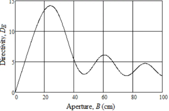
being dramatically reduced. Fig. 4 shows the variation of εap with the desired gain and Fig. 5 shows
the variation of te and t to the desired gain.
Fig. 4. Variation of the aperture efficiency obtained from the optimum design with a WR430 waveguide and a frequency of 2.5 GHz.
Fig. 5 Variation of the phase errors in the H-plane with respect to the desired gain obtained from the optimum design with a WR430 waveguide and a frequency of 2.5 GHz. −−− Exact phase error, − − − Quadratic phase error.
In the all designs, Cozzens’s method resulted in negatives values of the derivatives of the gain in
the H-plane. In Table IX, the derivative of the gain in the E-plane is also negative. This means that the
designed apertures passed the optimum point of design in the curve of directivity.
these equations, the same designs in Tables I, II and III were developed, whose results are shown in
Tables X, XI and XII. The analyses of these designs use (3) to (10) with (13) and (14).
TABLE X. RESULTS OF THE APPROXIMATED OPTIMUM DESIGN OF A PYRAMIDAL HORN ANTENNA WITH A GAIN OF 18dB USING A WR137 WAVEGUIDE AND A FREQUENCY OF 6 GHZ (λ =5 CM)
Approximated Optimum Design Design Dimensions Analyzed Parameters
R2 (cm) 18.20 se 0.267
R1 (cm)
B (cm)
19.94 14.20
te
ap
0.401 0.479 A (cm)
Rp(cm)
18.46 16.17
G (dB) 18
TABLE XI. RESULTS OF THE APPROXIMATED OPTIMUM DESIGN OF A PYRAMIDAL HORN ANTENNA WITH A GAIN OF 23dB USING A WR62 WAVEGUIDE AND A FREQUENCY OF 14 GHZ (λ =2.14 CM)
Approximated Optimum Design Design Dimensions Analyzed Parameters
R2 (cm) 25.97 se 0.264
R1 (cm)
B (cm)
27.21 10.89
te
ap
0.400 0.486 A (cm)
Rp(cm)
13.76 24.08
G (dB) 23
TABLE XII. RESULTS OF THE APPROXIMATED OPTIMUM DESIGN OF A PYRAMIDAL HORN ANTENNA WITH A GAIN OF 14dB USING A WR430 WAVEGUIDE AND A FREQUENCY OF 2 GHZ (λ =15 CM)
Approximated Optimum Design Design Dimensions Analyzed Parameters
R2 (cm) 19.87 se 0.275
R1 (cm)
B (cm)
22.68 26.88
te
ap
0.422 0.463 A (cm)
Rp(cm)
36.16 15.83
G (dB) 14
Verifying the results in Tables X, XI and XII, the results are the same as calculated numerically by
(17) to (22), except for a small difference in the B value for all cases, and in the R1 and A values for
short antennas. The values of teand seobtained using (23) and (24) are close to the results shown in
Tables VII, VIII and IX. Therefore, for the optimum design, these news proposed equations can be
used to design a pyramidal horn antenna.
V. CONCLUSIONS
Usually, design procedures for pyramidal horn antennas employ constant values for the quadratic
phase errors. This study showed that these values are not constant when using relations (18) and (19)
with the exact phase errors and equations (25) and (26). The variations depend on the desired gain of
the antenna. For long antennas, it can be assumed that the aperture efficiency is close to 0.49. For
short antennas, the efficiency can reach values as low as 0.42. It is also shown that the optimum
design proposed results in aperture dimensions larger than the method in [14], and in intermediate
REFERENCES
[1] W. L. Stutzman, and G. A. Thiele, Antenna Theory and Design, 2nd ed., John Wiley and Sons, 1998, pp. 300-314. [2] D. E Cozzens, “Tables Ease Horn Design,” in Microwaves, pp.37 -39, March 1966.
[3] K. Liu, C. A. Balanis, C. R. Birtcher and G. C. Barber, “Analysis of Pyramidal Horn Antennas Using Moment Method”, in IEEE Trans Antennas Propagat., vol. AP-41, pp. 1379-1389, October 1993.
[4] E. V. Jull, “Errors in the Predicted Gain of Pyramidal Horns” in IEEE Trans Antennas Propagat., vol. AP-21, pp. 25-31, January 1973.
[5] S. A. Schelkunoff, Electromagnetic Waves. New York: Van Nostrand Rheinhold, 1943, pp. 360-364.
[6] K. T. Selvan, “An Approximate Generalization of Schelkunoff’s Horn-Gain Formulas”, in IEEE Trans Antennas Propagat., vol. 47, pp. 1001-1004, June 1999.
[7] E. V. Jull, and L. E. Allan, “Gain of a E-Plane Sectoral Horn – A Failure of the Kirchhoff Theory and a New Proposal” in IEEE Trans Antennas Propagat., vol. AP-22, pp. 221-226, March 1974.
[8] W. T. Slayton, “Design and Calibration of Microwave Antenna Gain Standards” U.S. Naval Res. Lab., Washington, D.C., Rep. 4433, November 1954.
[9] J. L. Teo, K. T. Selvan, “On the Optimum Pyramidal-Horn Design Methods”, in Int J RF and Microwave CAE 16, pp.561-564, September 2006.
[10]M. J. Maybell, and P. S. Simon, “Pyramidal Horn Gain Calculation with Improved Accuracy”, in IEEE Trans Antennas Propagat., vol. AP-41, pp. 884-889, July 1993.
[11]K. T. Selvan, R. Sivaramakrishnan, K. R. Kini, and D. R. Poddar, “Experimental Verification of the Generalized Schelkunoff’s Horn-Gain Formulas for Sectoral Horns”, in IEEE Trans Antennas Propagat., vol. 50, pp. 875-877, June 2002.
[12]T. A. Milligan, Modern Antenna Design, 2nd ed., John Wiley and Sons, 2005, pp. 343.
[13]J. F Aurand, in “A New Design Procedure for Optimum Gain Pyramidal Horns”, in Antennas and Propagation Society International Symposium, AP-S Digest, 1988.