DEPARTAMENTO DE FÍSICA
PROGRAMA DE PÓS-GRADUAÇÃO EM FÍSICA
TATIANA MARÍA ALONSO AMOR
CHARACTERIZING AND MODELING VISUAL PERSISTENCE, SEARCH STRATEGIES AND FIXATION TIMES
CHARACTERIZING AND MODELING VISUAL PERSISTENCE, SEARCH STRATEGIES AND FIXATION TIMES
PhD thesis presented to the Post-Graduation Course in Physics of the Federal University of Ceará as part of the requisites for obtaining the Degree of Doctor in Physics.
Advisor: Prof. Dr. José Soares de Andrade Jr.
Co-Advisor: Prof. Dr. Hans J. Herrmann.
Gerada automaticamente pelo módulo Catalog, mediante os dados fornecidos pelo(a) autor(a)
A1c Amor, Tatiana María Alonso.
Characterizing and modeling visual persistence, search strategies and fixation times / Tatiana María Alonso Amor. – 2017.
114 f. : il. color.
Tese (doutorado) – Universidade Federal do Ceará, Centro de Ciências, Programa de Pós-Graduação em Ecologia e Recursos Naturais , Fortaleza, 2017.
Orientação: Prof. Dr. José Soares de Andrade Jr.
1. Busca visual. 2. Movimento Ocular. 3. Estratégias de Busca. 4. Caminhante Aleatório. 5. Distribuição de tempo de fixações. I. Título.
Deciding to pursue a PhD abroad is not an easy decision. It is a decision that forces us to leave everything we know, our home, our family, our friends, and ventures us into facing new challenges. These lines are to thank those who helped me making this possible.
First, I would like to thank Prof. José Soares de Andrade, Jr. for inviting me to do my PhD in Fortaleza and being my advisor. Thanks for introducing me to the wonderful group of people at the Complex Systems Lab and for allowing me to follow my own questions. My appreciation also goes to Prof. Hans Herrmann who granted me the opportunity to be part of his team at ETH. Thanks for being always available to discuss any project and, in this way, push me to work harder. I would also like to mention Prof. Antônio Gomes de Souza Filho and Prof. Alejandro Ayala whom have been extremely helpful over the past three years and have helped me with all sort of bureaucratic issues. I am also grateful to the Brazilian National Counsel of Technological and Scientific Development (CNPq) for the financial support.
A very special gratitude goes out to the Post-Doc dream team formed by Dr. Mirko Luković and (now) Prof. Saulo Reis. Thank you for being available to discuss science at any time and in any place. Thank you for guiding me when I needed help and for letting me pursue my own ideas without ever letting me on my own. Thanks for being involved in all the technical details of this thesis and for sitting down with me to teach me how to write (still learning!). Thanks for always being concerned about my academic future and for supporting my professional decisions.
Many thanks go to Heitor Credidio for being the first one to introduce me to the eye-tracker. All the analysis in this thesis concerning the WW and 5-2 cohorts wouldn’t have been possible without his personal belief that sharing data and information is the way science should work.
Damian, David, Konstantin and Kornel for their kindness and friendship. Thank you guys for making me fell welcome from the very first moment I entered the office.
es por eso que cuesta tanto trabajo encontrarlas.”
time, the candidate function to model the distribution needs to be the response of some very robust inner mechanism found in all the aforementioned scenarios. Hence, we discuss the idea of a model based on the microsacaddic inter event time statistics, resulting in the sum of Gamma distributions, each of these related to the presence of a distinctive number of microsaccades in a fixation.
delas são estatisticamente diferentes. Considerando que os tempos de fixações podem ser controladas por dois mecanismos diferentes: cognitivo ou ocular, focamos nossa pesquisa na busca de um modelo para a distribuição dos tempos de fixação suficientemente flexível para capturar os comportamentos observados em experimentos. Ao mesmo tempo, a função candidata para modelar a distribuição precisa ser a resposta de algum mecanismo interno muito robusto encontrado em todos os cenários acima mencionados. Assim, discutimos a idéia de um modelo baseado na estatística das microssacadas, resultando na soma de distribuições Gama, cada uma delas relacionada à presença de um número distinto de microsacadas contidas numa fixação.
Figure 1 – Schemes of the: eye’s anatomy, retinal cell organization and visual pathway. 26 Figure 2 – First indicators of a correlation between eye movement and cognition:
the Yarbus experiment. . . 31
Figure 3 – Eye-Tracker experimental setup . . . 38
Figure 4 – Calibration screen . . . 39
Figure 5 – Stimuli for the CN experiment. . . 40
Figure 6 – Stimuli for the 5-2 and WW experiment . . . 41
Figure 7 – Stimuli for the TrialDiff and ClickDiff cohorts . . . 42
Figure 8 – Stimuli for the online datasets . . . 43
Figure 9 – Definition of θh and θd . . . 46
Figure 10 – Eye-tracker raw and simplified data for the CN experiment . . . 46
Figure 11 – The distribution of the horizontal angle (θh) exhibits spatial anisotropy 47 Figure 12 – Directional persistence is unveiled by the distribution of the directional angle (θd) . . . 48
Figure 13 – The distribution of θh shows different strategies for the visual search . . 50
Figure 14 – The distribution of θd shows different strategies for the visual search . . 50
Figure 15 – Saccade velocity profile for the reading and non-reading like trials. . . . 51
Figure 16 – Short-term persistence on saccadic events . . . 52
Figure 17 – Magnitude gaze position time series and their integrated signal . . . 54
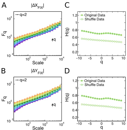
Figure 18 – Multifractal Detrended Fluctuation Analysis (MF-DFA) of the magni-tude position time series shows two scaling regimes . . . 56
Figure 19 – Stitching process for the fixation time series . . . 57
Figure 20 – Fixation time series exhibit a long-range positive correlated monofractal behavior . . . 58
Figure 21 – Different types of visual trajectories are found in the CN experiment . 60 Figure 22 – Schematic definition of the Visual Search Model (VSM) . . . 61
Figure 23 – Characteristic shape of the ranked inter-saccadic angles, θ, for the CN cohort . . . 62
Figure 24 – Validation of the VSM with the experimental eye paths . . . 63
Figure 25 – Example of a search where the VSM fails to predict the expected ε value 65 Figure 26 – VSM parameters for WW and 5-2 experiments . . . 65
Figure 27 – Validation of the VSM with the experimental trajectories from the WW cohort and the 5-2 cohort . . . 66
Figure 28 – Different tasks are placed in distinctive positions in the parameter space 67 Figure 29 – Parameters δθ and λ separated by trial index and subject . . . 68
Figure 32 – Fixation times probability distributions and cumulative distributions
for different visual tasks . . . 73
Figure 33 – Mean, standard deviation and skewness computed for the analyzed datasets . . . 75
Figure 34 – D and p-values from the two-sample Kolmogorov-Sminorv test . . . 76
Figure 35 – Possible fittings for the CN fixation times distribution . . . 78
Figure 36 – Fitting of the CN fixation time distribution by an exponentially modified gaussian and fitting parameters for all datasets . . . 79
Figure 37 – Probability distribution and higher order moments for the logarithm of the fixations times . . . 80
Figure 38 – Henderson & Pierce’s experiment: evidence for a mixed control for fixations duration . . . 82
Figure 39 – Example of a microsaccade . . . 84
Figure 40 – The distribution of the inter microsaccadic intervals follows an expo-nential distribution, evidencing a Poisson process . . . 85
Figure 41 – Synthetic fixations generated by the sum of two microfixations or ten microfixations . . . 86
Figure 42 – Synthetic fixation distribution generated with the sum of different Gamma distributions . . . 87
Figure 43 – MF-DFA over the increment time series . . . 104
Figure 44 – Distribution of values of the fixational time series . . . 105
Figure 45 – MF-DFA results for the rejection method sampling time series set . . . 106
Figure 46 – Hurst exponent for the magnitude time series with and without mi-crosaccades. . . 107
Figure 47 – Trajectories for the CN cohort. . . 109
Figure 47 – Continuation. . . 110
Figure 47 – Continuation. . . 111
Figure 47 – Continuation. . . 112
Figure 47 – Continuation. . . 113
2S-KS Two-Sample Kolmogorov-Sminorv test
5-2 Designation for the “5-2” cohort
CN Designation for the “Cloud-Number” cohort
cdf Cumulative Density Function
DFA Detrended Fluctuation Analysis
FTD Fixation Times Distribution
H Hurst exponent
MF-DFA Multifractal Detrended Fluctuation Analysis
pdf Probability Density Function
VSM Visual Search Model
1 INTRODUCTION . . . . . . . . . . . . . . . . . . . . . . . . . . . 25
1.1 The visual system. . . 25 1.2 Eye movements . . . 29 1.3 Eye movements and cognition . . . 30 1.4 Vision and memory. . . 32 1.5 Visual search strategies . . . 33 2 EXPERIMENTAL DESIGN . . . . . . . . . . . . . . . . . . . . . 37
2.1 Eye tracker device . . . 37 2.2 Experimental cohorts . . . 39
2.2.1 Cloud-Number experiment (CN) . . . 39 2.2.2 5-2 and Where’s Wally? experiment (5-2, WW) . . . 41 2.2.3 4 Differences experiment . . . 42 2.2.4 Public databases . . . 43
3 PERSISTENCE DURING VISUAL SEARCH . . . . . . . . . . 45
3.1 Geometrical persistence . . . 45
3.1.1 Reading and non-reading-like search strategies . . . 48 3.1.2 Short-range persistence on saccadic events . . . 51 3.1.3 Conclusion . . . 52
3.2 Statistical persistence . . . 52
3.2.1 Multifractal dentrended fluctuation analysis (MF-DFA) . . . 53 3.2.2 MF-DFA over the magnitude time series. . . 53 3.2.3 MF-DFA over the fixational time series . . . 55 3.2.4 Conclusion . . . 57
4 MODELING VISUAL SEARCH STRATEGIES . . . . . . . . . 59
4.1 The visual search model (VSM) . . . 59
4.1.1 Estimation of λ and δθ from the experimental data . . . 60
4.2 Efficiency map on the VSM parameters space . . . 62 4.3 VSM parameters in different visual search tasks . . . 64
4.3.1 Conclusion . . . 67
5 FIXATION TIMES . . . . . . . . . . . . . . . . . . . . . . . . . . 71
5.1 Similar but different . . . 71 5.2 Modeling the fixation times distribution . . . 76
experiment . . . 81 5.4 Microsaccadic statistics . . . 83
5.4.1 Combination of Gamma distributions . . . 84
6 DISCUSSION . . . . . . . . . . . . . . . . . . . . . . . . . . . . . . 89
BIBLIOGRAPHY . . . . . . . . . . . . . . . . . . . . . . . . . . . . . . . . . 93
ANNEX A PERSISTENCE DURING VISUAL SEARCH . . . . 103
A.1 Magnitude time series . . . 103 A.2 Magnitude distribution in the fixational time series . . . 104 A.3 Microsaccadic movements in the magnitude fixational time series105
1 Introduction
Almost 60% of our brain is involved in processing visual information. For humans and many other species is through vision that we acquire most of the information from the world around us. Hence, pursuing to understand vision puts us a step closer into comprehending the process that brings us much of our knowledge.
In our everyday life we gather visual information from the world around us by performing a vast variety of visual tasks. Let us think of an oversimplified example to explain some of these visual tasks: taking out a book from the library. First, we take the bus to the university library, on the ride we look at the city through the bus window (free viewing), we see a friend sitting at the back of the bus (face recognition), we wave at him, he seems happy (emotion recognition), he is going to the university too. When we arrive at the university we go to the library building (object recognition), and ask the librarian for the book at issue. We glance through the library shelves looking for it until we find it (visual search). We sit down with the book in front of us and recognize the letters inside it (pattern recognition), we take a deep breath and focus on understanding what is written (reading).
In this thesis we propose to study these visual tasks from a physicists perspective. In what follows we describe the physiology of the visual system, from the eye to the visual cortex. Then, we introduce the main topic of study of this thesis, the eye movements. We review how these movements relate to cognition and focus into one particular visual task: visual search. We review what is known from the literature regarding visual search as an optimal setting to study visual memory and search strategies. Finally, we present the current notions related to fixation times, beyond visual search.
1.1 The visual system
The visual system is formed by the eye, with its inner structures, and the brain regions involved in the visual pathway towards the visual cortex. Six small extra-ocular muscles control the motion of the eyeball, for each one of our eyes. These muscles consist of three pairs, each pair working in opposition. Any eye movement is made by contracting one muscle and relaxing its opponent by just the same amount. Having six muscles for each eye is necessary, as each pair takes care of movements in one of three orthogonal planes. Going inside the eye itself, Fig. 1. We find the cornea, the transparent part of the eye, and lens both responsible for focusing light rays onto the back of the eye. About two-thirds
is to focus objects at various distances. This last is done by changing the shape of the lens by pulling or relaxing the tendons that hold it at its margins. The amount of light entering the eye is regulated by another set of muscles that change the diameter of thepupil. In
addition, the eye counts with a self-cleaning process obtained by closing the lids (blinking) and lubricating the eye with tear glands. Interestingly, the cornea is richly supplied with nerves related to touch and pain, so the slightest irritation sets up a reflex that leads to blinking.
Left Visual
Field
Right Visual Field
Optical lens
Retina
Optic nerve
Optic chiasma
Lateral geniculate nucleus (LGN)
Primary visual cortex
Visual Pathway
T
h
e
E
y
e
Optic nerve Retina
Lens Pupil
Cornea Iris
Fovea
R
eti
n
a
l
Or
g
a
n
iz
a
ti
o
n Cone Rod
Bipolar cell Ganglion cell
Pigment epithelium Amacrine cellHorizontal cell
Figure 1 –Schemes of the: eye’s anatomy, retinal cell organization and visual pathway.
(The Eye) Scheme of the eye with its internal structures. The cornea and the lens are responsible for focusing the light rays onto the back of the eye, the retina. By modifying its shape the lens serve as a way to focus objects in different distances. (Retinal Organization) Schematic insight of the cells found in the retina and its organization. The last layer is composed by the light
receptors, rodes and cones. The middle, by the horizontal cells, bipolar cells and horizontal cells. The first layer, by the retinal ganglion cells that converge into the optic nerve and send the visual information into the brain. This cross section of the retina corresponds to somewhere between the fovea and the periphery where there is equal density of cones and rodes. (Visual Pathway)
Visual pathway of a human brain as seen from below. Information goes from
the retina into the lateral genicualte nucleus and then into the visual cortex. Information gathered from both eyes travels into the right lateral genicualte (orange lines) and into the left lateral genicualte (blue lines).
Source: Elaborated by the author using (STAFF, 2014; HUBEL; WENSVEEN; WICK, 1995; NIETO, 2015) as references.
All these structures exist in the interest of theretina, responsible for translating
detect fine detail in objects. The output from the retina converges into the optic nerve that then sends information into the brain. The retina consists of three layers of nerve-cell bodies (Fig. 1.Retinal Organization). The last layer of the retina is composed by light receptor cells namely, rods and cones. Rods, are far more numerous than cones and relate
to vision in dim light. Cones are responsible for our ability to see fine detail and for our color vision. In the very center of the retina our vision has its most acuity region, where mainly cones are present. This area is called the fovea.
At this point, it is important to note that the retina is developed in a backward fashion so that, a beam of light needs to pass the first and second layer of the retina up to the third layer in order to stimulate the light receptors, and then go backwards to create a response. This, somehow, counterintuitive layout of the retina is yet not fully understood. Research on the area suggests that a possible reason for this layout is due to the presence of pigmented epithelium cells located behind the photoreceptors (STRAUSS, 2005). These
pigmented cells containing melanin help to avoid back reflections and scattering of the beams of light entering the eye. Furthermore, the pigmented epithelium cells contribute into restoring the light-sensitive visual pigment in the photoreceptors after the beam of light has first stroke them (photo-oxidation). These functions require the pigment epithelium cells to be placed near the receptors. Perhaps, naively, one would expect the photoreceptors to be located in the first layer of cells of the retina, if this would be the case, then the melanin-containing cells would need to be immediately after in a region already packed with axons, dendrites, and synapses.
Moving backwards into the retina we find the middle layer, composed bybipolar cells,horizontal cells and amacrine cells. The first layer of the retina is composed by the
retinal ganglion cells, with axons passing across the surface of the retina and leaving the
eye to form the optic nerve. The bipolar cells have their input taken from the receptors and many of them have their output sent into the retinal ganglion cells. Horizontal cells link receptors and bipolar cells and amacrine cells link bipolar cells and retinal ganglion cells (DOWLING, 1987; KUFFLER, 1952; NICHOLLS et al., 1992).
In and near the fovea the direct path works feeding from one single cell into another, that is, one receptor feeds one bipolar cell that then feeds only one ganglion cell. Hence, visual information falling into the fovea region is “seen” with high detail. As we go farther out from the fovea, the situation differs as more receptors converge on bipolar cells and more bipolar cells converge on ganglion cells. Having a high degree of convergence far away from the fovea and a very low degree of converge on the fovea helps to understand why although having this ratio of different cells we do not have a poor vision. For an extensive review on retinal organization and retinal cells, please refer to (WÄSSLE, 2004).
When the optic nerve leaves the eye and goes into different brain structures it does in a well organized way. The fibers leaving from the optic nerve go into a lateral structure of the brain calledlateral geniculate nucleus. The fibers corresponding to the right half of the right eye go to the right geniculate and the fibers corresponding to the left half of the left eye go to the left geniculate. In addition, the left half of the right eye goes into the left genicualte and the right half of the left eye goes into the right genicualte, all crossing at theoptic chiasm, as depicted in Fig. 1.Visual Pathway. Thus, both hemispheres
receive information on the visual scene perceived from both eyes. The optic nerve fibers gather into a bundle as they leave the eye and, when they reach the lateral genicualte nucleus, they fan out in a topographically orderly way. Between the retina and geniculate they are almost completely scrambled, but when reaching the geniculate they sort out. The fibers that leave the lateral genicualte then go through the interior of the brain until reaching theprimary visual cortex (V1). This then communicates with other visual ares called V2, V3, V4 and V5, also known collectively asextrastriate visual cortex.
The primary visual cortex (V1) is highly specialized for processing information about static and moving objects and is excellent in pattern recognition. The fast neuronal response in V1 (at about 40ms) is able to discriminate small changes in visual orientation, colors and spatial frequencies. After 100ms of having received the visual input from the retina, the neurons in V1 are able to distinguish aspects related to the global organization of the scene (LAMME; ROELFSEMA, 2000). These response could be due to recurrent feedback sent from higher-order cortical areas which can modify and shape V1 neural activity (SILLITO; CUDEIRO; JONES, 2006; XU et al., 2007).
the human brain at a large spatial scale in a non-invasive manner (GRILL-SPECTOR; MALACH, 2004).
1.2 Eye movements
In any visual task we are constantly gathering information from the scene we contemplate, while performing high-speed eye movements, called saccades, towards
potential target positions (LIVERSEDGE; FINDLAY, 2000). The steps in between these saccades namely, the fixations, allow us to inspect the scene at high-resolution as these
images fall into the central retina (HUBEL; WENSVEEN; WICK, 1995), the fovea, where the convergence of the photoreceptors into the ganglion cells is lower, as discussed in Section 1.1. The fixations are therefore the events during which most visual information is captured from the target positions or from the scene (INHOFF; RADACH, 1998). This sequence of fixations and saccades is what mainly constitutes the eye trajectories with which we will be dealing along this work.
In addition, during the fixations a series of inner small ocular movements carry the image across the retinal photoreceptors. These movements are classified as: tremor, drifts and microsaccades. The first one corresponds to the smallest of all eye movements,
there is not a consensus, yet, of their contribution to the visual system and perception. Some studies suggest that this type of motion appears in order to correct the position of the eye when drifts displace the target from the fovea and to reduce retinal fatigue, preventing fading (CORNSWEET, 1956). At the same time, microsaccades which do not perform this task also appear (FIORENTINI; ERCOLES, 1966). Within this lines, it was suggested that microsaccades serve to correct fixation error on a longer timescale (ENGBERT; KLIEGL, 2004). Moreover, microsaccades were also associated to play a role in perceiving hue differences at low contrast (DITCHBURN, 1980). Later, microsaccades were related to the firing variability of neurons in V1 (GUR; BEYLIN; SNODDERLY, 1997). Please refer to (SCHÜTZ; BRAUN; GEGENFURTNER, 2011; MARTINEZ-CONDE; MACKNIK; HUBEL, 2004) for a review on fixation movements.
Up to here we have discussed eye movements in humans with well functioning extraocular muscles. One could then ask, what would happen to someone with a muscular disability. Would this have an influence in its visual perception? In 1997 a clinical case of a 21 year old female (A.I.) with extraocular muscular fibrosis was studied to shed light into this question (GILCHRIST; BROWN; FINDLAY, 1997). Researches found that her visual perception was normal and tested her on a reading task. Her reading time was within normal times and, more interestingly, they found that the typical saccadic movements performed while reading were compensated in A.I. with head movements. Her head movements followed the same saccadic fashion as eye movements. They were fast and allowed her to fixate in similar positions in the text as people with normal vision. Hence, even though she was unable to move her eyes, the head played the role of the extraocular muscles and moved her eyes towards possible regions of interest. Given that A.I. did not develop other strategy to scan the world around her suggests that saccadic movements form the optimal exploration method for the brain.
Along this work we present a study of these ocular movements from different perspectives. In Chapter 3 we studied the fixations and saccades through the analysis of their associated time series. Trough the study of the saccadic movements, we studied the emergent trajectories during a visual search task, in Chapters 3 and 4. In Chapter 5, we focused our study on the time elapsed during fixation for various visual tasks.
1.3 Eye movements and cognition
its pinnacle with the publication of the book Eye movements and vision first published in
Russian in 1965 and translated to English in 1967 (YARBUS, 1967). Interestingly, it was only after the English edition of his book that Yarbus became a well known researcher on the western scientific world (TATLER et al., 2010). Even though his work focused mainly on providing new technologies to track eye movement, his most influential work was the study of the cognitive influences on scanning patterns. Since then, his study, comprising only one chapter of his book, has had a massive impact on research on eye movement in particular, and on the visual system in general.
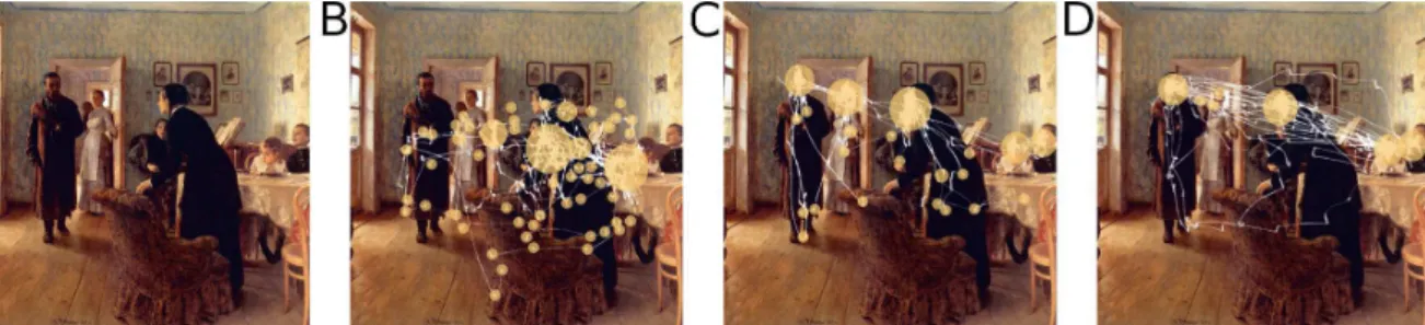
Figure 2 – First indicators of a correlation between eye movement and cognition: the Yarbus experiment. Yarbus showed a painting ((A) Ilya Yefimovich Repin’s
‘The Unexpected Visitor”) to its participants and asked a set of questions. Some of his questions were: to estimate the socioeconomic condition of the characters, (B), how old they were(C) and how long had the visitor been away (D). The
eye paths differ from one question to another showing a correlation within the eye trajectories and the cognitive task. The yellow dots represent the locations where fixations are present.
Source: Adapted by the author from (ARCHIBALD, 2008).
Yarbus studied how the visual scanpaths change while inspecting the same image under different experimental directions. He asked one participant to look at a painting from the artist Ilya Yefimovich Repin called The Unexpected Visitor(Fig. 2A)
1.4 Vision and memory
As discussed in the previous section, eye-movement data provides information on the cognitive process underlying visual tasks. In particular, so it does for visual search tasks which can be used to shed some light on how the human (or animal) eye implements information for foraging and/or planning (ARAUJO; KOWLER; PAVEL, 2001; BOCCIGNONE; FERRARO, 2004; OVER et al., 2007). A number of studies have been conducted on the visual search of hidden objects in complex scenes (RAO et al., 2002; CREDIDIO et al., 2012; OTERO-MILLAN et al., 2008), going from cases of targets embedded in a noisy background (NAJEMNIK; GEISLER, 2005) to more simplified visual tasks on macaques (MOTTER; BELKY, 1998). Visual search, however, remains a complex cognitive task which involves a number of diverse underlying mechanisms that need to be addressed. One of these essential mechanisms, whose properties are still under debate, is memory.
The first theories on visual search assumed the existence of visual memory in terms of an inhibitory mechanism that prevents an item to be revisited after identifying it as a distractor (TREISMAN; GELADE, 1980), or in the capacity of collecting visual information in parallel for each item inspected (PALMER, 1995). Later, it was suggested that visual search involves a memoryless search strategy (HOROWITZ; WOLFE, 1998). By studying the response time of a visual task involving the search of a target along with distractors, it was found that the efficiency of search remains constant across trials. This would imply that the visual system does not accumulate information about an item over time during a search episode and that subjects may frequently reinspect locations that have already been inspected. However, although subjects tend to reexamine some items, the pattern of revisitations does not match the one predicted by a memoryless model (PETERSON et al., 2001). Thus, it has been argued that revisitations occur not because the searcher forgets the items that have been examined, but because the items were inadequately examined at first. So, while memory may not be a primary mechanism for instantaneous object recognition (in these scenarios saliency could be, for example, more significant (COSTA, 2006; BROCKMANN; GEISEL, 2000)) it seems clear that it must play a role in cognition and, in particular, in strategy planning. Along these lines, the problem of visual memory has been recently addressed as a synonym of persistence for natural scenes in a number of works (MELCHER, 2001; MELCHER; KOWLER, 2001; MELCHER, 2006). From the study of how subjects can recall unrelated items, removing semantic cues, it has been shown that visual memory over time performs better than had been thought. Therefore, persistence may represent a convenient conceptual measure to analyze the performance and/or efficiency of living beings performing real-world visual tasks.
through the analysis of purely cognitive measurements, such as the response time of subjects or the amount of objects recalled after inspecting a scene. In this thesis we address the question: Is there any quantifiable persistent behavior in the visual trajectories during visual search?
In Chapter 3 we disclose that the process of eye movement during visual search exhibits two distinctive persistent behaviors. Initially, we condense the information about the eye paths by reducing fixations and saccades to a set of points and vectors, respectively. First, our results reveal that the probability distributions of the angles between the intersaccadic vectors present a clear asymmetry which indicates the existence of a short-range geometrical persistence related to a reading-like strategy of search, discussed
in Sections 3.1. Second, we apply the Multifractal Detrended Fluctuation Analysis method (MF-DFA) to study the whole time series of eye movement during visual search, which encompasses fixations as well as saccades. In Section 3.2, we show that this sequential combination of distinct events leads to an apparent multifractal signature. Moreover, by inspecting the time series composed only of fixational movements, we observe that it presents instead a monofractal behavior, which is indicative of the presence of long-range power-law positive correlations. Such power-law correlations are synonymous of long-range statistical persistence and therefore are interpreted as a signature of long memory
processes (BAILLIE, 1996).
As mentioned before, both approaches (geometrical and statistical) are not direct cognitive measurements, as they just arise from the analysis of the visual path. By making direct measurements on the eye paths we are able to address how visual search is performed from a different perspective.
1.5 Visual search strategies
The study of visual search experiments lead to a natural subject of investigation: the searching strategies employed by participants while looking for a hidden target. Hence, we can ask ourselves what visual strategy do we employ when searching for a familiar face in a crowd and how would it change if we had to find a friend in a well organized choir? For instance, do we explore each face sequentially or do we pick them randomly until reaching our target. Along these lines, it is not at all obvious whether there exists a characteristic strategy that is related to the scene content. To shed light onto this problem it is necessary to find a method that allows us to identify and quantify particular features associated to the strategy adopted.
Different models have been developed with the goal of understanding what guides eye movement during visual search (see (ECKSTEIN, 2011) for a review). One family of these models is based on the construction of saliency maps, which define
orientation) (ITTI; KOCH; NIEBUR, 1998; ITTI; KOCH, 2000; OVER et al., 2007; FOULSHAM; UNDERWOOD, 2008; EHINGER et al., 2009; NAKAYAMA; MARTINI, 2011). By definition, these salient regions stand out from other parts of the scene and are therefore more susceptible to frequent eye fixations. In the context of visual search, these models prove to be more suitable for tasks involving a small number of equally relevant distractors, which are essentially all items in the scene that are not targets of the search (LI, 2002; SHIFFRIN; GARDNER, 1972). On the other hand, in more complex visual search tasks, the salient regions might not necessarily be relevant. In order to address this issue, other implementations of the saliency model consider the relative information of an object with respect to the global information of the scene (ZHANG et al., 2008; BRUCE; TSOTSOS, 2009; GAO; HAN; VASCONCELOS, 2009).
In the absence of salient elements, it is not possible to use these models as there are no a priori privileged regions within the scene. As a consequence, another
family of visual searching models have been proposed, namely, thesaccadic targeting mod-els (RAO et al., 2002; BEUTTER; ECKSTEIN; STONE, 2003; ECKSTEIN; DRESCHER;
SHIMOZAKI, 2006; POMPLUN, 2006; ZELINSKY, 2008). In these studies, the main hypothesis is that saccadic eye movements are directed to locations within the scene that contain elements similar to the target. This similarity can be due to the image content as well as to a neurobiological filter. Within this framework, Najemnik & Geisler propose a model where each point in space has a certain probability of being explored and the saccadic movement is directed to the most probable regions (NAJEMNIK; GEISLER, 2005; NAJEMNIK; GEISLER, 2008). These probabilities are then updated over time so that regions that were already explored are less likely to be revisited, introducing in a natural way the notion of persistence while searching. Moreover, other implementations of this model have taken into account the proximity between consecutive saccadic movements by adding a cost function that punishes longer saccades (ARAUJO; KOWLER; PAVEL, 2001).
the sequence in which the fixations are performed but instead determine the regions where they are more likely to occur. On the other hand, the saccadic targeting models, although dealing with the saccadic sequence, do not account for different strategies.
2 Experimental design
The experimental data analyzed through out this thesis corresponds to the recording of the eye movement while performing a visual task. Different eye-tracking devices use different techniques to record the ocular movement. Regardless of the device employed to record data, the eye movement data is composed of a list of positions, for example pixels, with a time step determined by the acquisition frequency of the equipment. In this chapter we explain the specifications for the equipment used in this work, the EyeLink 1000 system (SR Research Ltd., Mississauga, Canada), and give a description of the experimental cohorts studied.
2.1 Eye tracker device
We used the EyeLink 1000 system (SR Research Ltd., Mississauga, Canada) to track the movement of the eye while participants performed visual search tasks. This eye-tracking device comes with many different setup options, which allow to perform a diverse variety of experiments, from common laboratory use to highly sensitive EEG, MEG and MRI environments. It consists of a core system that can be used with different mounting options, with the Desktop option being the one used in our laboratory. This
mounting option allows us to record data in a non-invasive manner, as there are no electronic devices near the participant’s head.
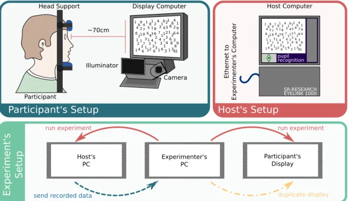
Figure 3 shows the basic experimental setup for any type of common laboratory experiments. The participant rests his/her head on a head rest which allows him/her to be in a comfortable position while performing the experiment and avoids undesirable head movements. The head rest is set at approximately 70cm of the participant’s screen, as specified for this eye-tracker device. Below the participant’s screen is located the high-speed camera and low output illuminator module. This module tracks the movements of the pupil and cornea reflection thus, the eye movement. The EyeLink 1000 allows to record eye movement with several sampling rates and in two modes: monocular (following only one eye) or binocular (following both eyes). The sample rate for a monocular recording can be 250, 500, 1000 or 2000Hz and 250, 500 or 1000Hz for the binocular mode. The eye movements are then mapped into locations on the screen through a previous calibration of the participant.
the experiment once it has ended. Host Computer E th er n et to E x p eri men ter' s Co mp u ter run experiment run experiment Display Computer Participant Head Support ~70cm Camera Illuminator 1 4 8 1 2
694
7 8 2 1
217
3 4
1 6 6
1 5 6 3
1
812
8 6 4 1
347
3 2 3 6 4 3 7 1 4
16 2
3 2 1 4
374
1 6 1 3 1 8 1 6 2
641
9 4 2 6
839
6 3 1 1 2 3 3 3 1 pupil recognition SR-RESEARCH EYELINK 1000
Participant's Setup Host's Setup
E x p eri men t' s S etu p 1 4 8 1 2 694
7 8 2 1
217 3 4
1 6 6
1 5 63
1 812
8 6 4
1 347
3 2 3 6 4 3 7 1 4 162 3 2 1 4
374 1 6 1 3 1 8 1 6 2 641
9 4 2 6
839 6 3 1 1 2 3 3 3 1 Host's PC Experimenter's PC Participant's Display duplicate display
send recorded data
Figure 3 –Experimental setup scheme. (Participant’s Setup)The participants sits at
approximately 70cm from the Display Computer. His or her head rests on a
head support which allows the participant to be comfortable and at the same time, maintains the head position fixed. The camera that collects the image of the eye is set in front of the Display Computer. (Hots’s Setup) The Host Computer is the EyeLink itself. On its screen appears the information regarding
the recording options of the eye and shows the eye movement in real time when performing an experiment. (Experiment’s Setup) The experiments are build on the Experimenter’s PC. The screen of the Experimenter’s PC is duplicated on the Participant’s Display to run the experiment. From the Experimenter’s PC one runs the experiment to the Host’s and Participant’s PC. On the Host’s PC all camera setups and calibration are performed. While running the experiment, the data is recorded on the Host’s PC. Once the experiment has finished, the recorded data is sent to the Experimenter’s PC.
The Experimental setup is composed by the Host’s PC, the Experimenter’s PC and the Participant’s display. The screen on the Experimenter’s PC is duplicated on the Participant’s display, so when running the experiment the participant and the experimenter are presented with the same stimuli. The experiment is run from the Experimenter’s PC which then communicates to the Host’s PC and, as it has already been mentioned, records and sends the experimental data back to the Experimenter’s PC.
or 13-point calibration. In the case of the 9-point calibration the black point appears in the center, corners and middle outer locations of the screen. For each fixation a cross appears on the Host’s screen. If the 9 crosses are arranged in a lattice, then the calibration is considered to be successful. On the other hand, if any deviations from a lattice appear, then the calibration is disregarded and a new calibration needs to be performed. The 13-point calibration is analogous to the 9-point calibration with four extra points located in the center point from the center of the screen to the corners.
+
+
+
+
Participant's screen Host's screen
Figure 4 – Eye-Tracker calibration.The calibration stage consists in asking the participant
to fixate his or her eyes at one point on the screen (Right). This point moves to different positions on the screen after a fixation on it has been recognized. While doing so, on the Host’s screen (Left) a cross appears on a location related to the fixated point. The cyan cross denotes the current point at which the participant should be fixating. The EyeLink 1000 allows us to perform a 9 or 13 point calibration. For the 9-point calibration the crosses are displayed in a three by three grid. The calibration is successful when there are no deviations from the grid. The 13-point calibration is analogous to the previous one, with four extra points between the center and the corners.
2.2 Experimental cohorts
What follows is a detailed description of the experimental data used in this thesis. All the experiments conducted at the Universidade Federal do Ceará have been approved by the Ethics Research Committee of the Universidade Federal do Ceará (COMEPE) under the protocol number 056/11. Informed consent was obtained from all subjects. All subjects had normal or corrected to normal vision.
2.2.1 Cloud-Number experiment (CN)
experimental sessions is depicted in Fig. 5.The numbers are first distributed on the image over a grid and then shifted a random distance from the grid’s node location. This results in a structure that resembles a lattice with some deviations.
Each subject carried out a sequence of four trials. For each trial, i.e stimuli, the participant was allowed to search for the unique number “5” for up to 5 minutes. Between each trial, the subject had the possibility to relax and before starting the recording we performed a new calibration. At the beginning of each trial, the participant was asked to fixate his/her eyes on the center of the screen, in case a drift correction needed to be performed. 48 3 7 9 2 7 8 8 3 8 7 3 6 2 2 3 76 6 2 3 7 2 7 8 2 6 4 2 7 9 4 2 6 9 7 3 3 1 1 8 6 4 6 6 7 4 8 3 1 9 1 8 7 1 1 4 3 9 7 6 7 8 7 1 2 8 8 1 7 2 4 8 9 64 9 9 1 7 3 8 9 6 6 8 13 1 1 4 4 4 4 7 6 9 4 4 6 3 18 9 6 6 3 7 7 6 3 2 2 28 9 1 7 7 4 1 4 7 8 8 6 3 8 1 99 3 1 8 8 5 1 6 33 8 8 6 2 4 4 86 7 3 1 2 7 8 1 2 4 9 1 7 1 7 9 8 8 4 3 7 6 4 4 7 8 7 2 3 2 2 9 6 6 6 7 2 1 1 9 9 6 2 7 4 4 7 9 36 8 8 6 9 2 8 4 2 6 9 6 9 2 9 2 39 8 8 7 6 6 2 9 1 8 1 7 3 4 8 9 49 9 2 4 83 6 7 4 8 1 2 7 3 7 1 4 42 3 8 24 8 33 2 7 4 4 4 7 72 33 1 6 8 1 3 9 2 2 2 8 2 4 8 6 4 8 8 8 3 7 2 6 6 4 2 3 1 6 1 4 7 4 3 4 4 17 1 6 7 8 9 4 3 8 1 4 4 7 6 4 9 2 9 1 1 2 2 3 7 7 6 6 7 7 97 1 8 1 1 2 1 6 3 2 1 6 7 6 9 6 1 7 4 1 9 6 2 2 2 6 6 8 3 8 6 2 8 6 8 4 7 1 3 7 7 8 9 6 8 3 4 9 1 2 2 1 9 96 9 9 7 7 8 6 4 7 86 88 9 7 4 6 4 8 2 3 7 7 6 2 99 6 7 3 9 3 6 9 3 4 1 8 1 9 9 2 14 4 2 6 9 7 3 7 7 8 2 2 2 3 1 2 7 6 1 8 8 1 6 2 1 7 1 4 7 2 2 1 2 6 4 1 6 1 7 3 21 8 7 6 6 1 8 3 2 1 9 1 7 6 8 8 6 1 2 1 8 2 2 9 3 6 7 2 67 7 6 8 7 8 6 2 6 3 48 9 1 3 3 2 9 1 2 4 13 8 7 7 1 6 7 8 4 9 8 1 8 3 3 7 1 1 2 1 3 9 6 8 9 7 7 9 1 9 24 6 6 4 8 1 8 1 3 8 2 8 8 3 3 3 3 4 14 26 8 6 2 6 9 3 6 9 46 6 2 1 2 1 9 1 98 9 3 44 7 2 6 44 3 3 2 8 4 1 1 1 2 2 4 9 9 1 1 3 9 9 1 6 2 9 1 8 92 2 8 9 9 4 9 2 7 9 38 6 1 3 6 7 7 7 2 9 3 6 2 7 3 6 3 1 6 9 1 2 8 1 7 4 3 2 4 2 18 2 3 7 7 9 9 3 2 3 7 8 8 2 6 3 6 7 7 3 6 3 2 2 9 7 8 4 6 12 8 4 2 7 8 9 9 4 9 8 7 6 3 1 4 8 1 4 6 6 7 8 7 1 9 1 1 6 2 7 7 8 1 7 3 2 8 7 3 1 7 1 7 3 9 4 3 4 2 6 1 6 7 88 9 9 2 6 9 3 7 1 2 24 4 2 9 9 6 1 8 6 6 4 6 9 7 7 44 2 8 2 6 7 46 7 8 3 1 88 7 7 9 9 2 44 6 7 1 38 8 6 9 6 1 1 4 8 6 7 3 3 1 8 2 26 3 7 3 6 14 4 31 1 3 8 9 2 4 6 6 1 1 9 4 1 9 2 3 4 1 9 6 4 6 9 2 3 9 1 3 6 4 28 9 3 6 3 3 1 2 8 2 8 6 1 3 1 84 6 9 2 4 6 7 6 3 2 1 2 9 7 2 3 9 2 9 2 92 12 1 4 4 3 9 1 9 6 8 1 6 7 8 7 8 78 4 6 2 8 92 6 2 1 9 9 1 7 8 7 8 6 1 1 3 1 9 7 2 4 7 7 3 7 4 3 8 1 4 8 6 2 9 2 2 26 8 3 6 2 1 3 7 3 1 7 3 2 4 9 2 1 7 8 83 7 1 91 6 9 1 6 2 29 9 4 4 1 4 3 2 9 7 1 73 2 7 8 8 7 2 27 2 8 9 6 4 6 6 8 3 4 7 4 8 4 4 4 8 1 9 3 6 6 7 9 2 9 8 8 6 4 2 2 9 2 9 7 3 2 3 3 2 9 9 6 1 2 4 9 9 9 8 4 4 3 1 3 8 7 7 7 2 9 6 8 4 3 8 4 8 3 9 6 9 1 6 4 9 1 9 6 82 7 2 91 9 3 2 1 2 7 9 1 9 8 9 9 63 8 9 7 7 4 8 2 9 1 2 2 4 6 2 9 8 8 4 8 3 9 4 1 82 4 3 9 3 6 3 2 7 9 1 97 2 7 9 96 7 8 6 9 4 8 48 2 3 6 8 6 2 4 9 6 3 1 9 1 7 7 7 1 1 9 8 3 8 1 7 2 1 1 4 7 7 2 72 2 4 4 3 2 9 2 1 1 3 1 7 2 1 8 7 6 1 14 1 23 1 7 6 2 6 1 7 3 7 3 4 9 82 8 9 8 6 22 7 4 7 4 3 1 2 2 61 9 4 2 3 9 6 1 1 7 8 1 9 6 8 2 6 2 3 3 6 2 2 7 9 2 2 6 9 98 31 6 9 4 3 3 4 4 8 3 3 1 1 11 7 4 9 7 1 7 3 1 9 2 2 7 8 6 7 9 1 9 2 2 4 97 2 6 2 7 76 7 8 8 6 8 8 4 9 1 4 9 9 4 21 3 83 8 2 4 7 9 2 1 2 8 3 2 7 8 1 8 2 86 7 7 4 3 3 6 7 8 3 1 9 6 6 7 2 2 6 8 7 3 6 2 3 3 1 9 21 6 6 24 3 2 7 9 9 2 1 1 2 3 4 2 7 3 7 7 2 61 6 8 8 2 8 83 12 3 3 3 7 8 9 2 1 27 7 4 4 6 9 9 3 7 6 7 7 2 72 4 9 94 1 7 3 2 8 6 6 7 6 31 23 4 1 4 2 6 6 1 8 4 22 8 9 6 4 9 7 6 6 1 9 9 3 3 2 3 2 2 4 8 8 2 61 82 6 1 4 3 3 8 7 7 1 2 7 1 9 4 4 7 1 2 3 6 2 8 7 38 6 4 2 8 3 1 3 6 4 1 7 3 2 2 2 7 4 3 3 44 6 22 7 3 9 4 3 1 8 7 7 6 7 1 6 88 4 6 9 9 4 2 8 7 9 7 4 7 1 2 7 3 8 8 8 2 6 4 2 4 7 9 2 9 2 9 3 7 2 31 3 6 6 9 2 8 7 2 7 7 4 3 9 8 2 3 9 4 3 3 9 8 79 6 1 13 2 7 9 2 2 8 8 2 7 4 1 3 3 8 6 2 7 8 49 6 3
Figure 5 – Stimuli for the CN experiment.
The experimental data corresponding to the CN cohort was recorded with the EyeLink 1000 system (SR Research Ltd., Mississauga, Canada) described in the previous section, with an acquisition frequency of 1kHz on a monocular recording. Ten graduate and under-graduate students (mean age: 24) participated in this study.
acceleration of the eye using fixed thresholds for both eye velocity and acceleration. If the eye goes above either the velocity or acceleration threshold, the start of a saccade is marked. Analogously, when both the velocity and the acceleration drop back below their thresholds, the algorithm identifies the saccade end. By default, every movement which does not lie within this definition is considered as being part of a fixation. The saccade velocity threshold was set to be 30◦/s, the saccade acceleration threshold, 8000◦
/s2, and
the saccade motion threshold, 0.15◦.
The CN cohort was used for the studies explained in Chapters 3 and 4. The fixation time distribution is analyzed in Chapter 5. The data corresponding to this cohort can be access online at figshare.com/s/9e2b1d3545dd04e44d94.
2.2.2 5-2 and Where’s Wally? experiment (5-2, WW)
The 5-2 experiment consists in finding a number “5” within an array of numbers “2” serving as distractors. All numbers (target and distractors) are positioned on a square lattice and are randomly colored red or green, hindering the visual detection of the target through the identification of patterns on the peripheral vision, as depicted in Fig. 6. The number of distractors present in each task is related to the degree of difficulty: DF0 (207 distractors), DF1 (857 distractors) and DF2 (1399 distractors). The maximum time given to search for the target was 1, 1.5 and 2 minutes respectively.
Figure 6 –Stimuli for the 5-2 (Left) and WW (Right) experiment.
Source: Figure of the WW stimuli: (HANDFORD, 1997)
The WW experiment consists in finding “Wally”, the famous character from
the series of books with the same name (HANDFORD, 1997), who is hidden within a very complex background of crowded characters (see Fig. 6), with a maximum searching time of 2 minutes.
subjects (mean age: 23). The stimuli were presented on a 17” TFT-LCD monitor with resolution 1024×1280px and acquisition frequency of 60Hz.
As explained in (CREDIDIO et al., 2012) the identification of fixations and saccades was carried out with a modified version of the fixation filter developed by Olsson (OLLSON, 2007).
The 5-2 and WW cohorts are analyzed in Chapter 4 of this thesis. Also, the distribution for the fixation times is analyzed in Chapter 5.
2.2.3 4 Differences experiment
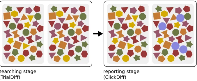
For the 4 Differences experiment we generated images where the participant is asked to find and report the four differences encountered within two subfigures (see Fig. 7). Each image is composed by several items each of which can correspond to an element within a set of seven different shapes. These shapes are polygons which can be differentiated under rotations. Moreover, the shapes are presented in five possible colors. The possible differences are classified in three categories: color, shape or rotation. Each participant is presented with one image for each category for two system sizes, approximately 100 and 200 items respectively.
searching stage (TrialDiff)
reporting stage (ClickDiff)
Figure 7 –Stimuli for the 4 Differences experiment. The experiment consist of two stages.
In the first one the participant is indicated to search and find the four exist-ing differences in the image, searchexist-ing stage (Left). In the second one the participant is indicated to report where the differences are by clicking on the different shape found. After doing so, a circle appears on the region that has been clicked, reporting stage (Right).
he or she must indicate where the differences are by clicking on the odd shape in one of the subfigures. We will refer to this cohorts as TrialDiff and ClickDiff, respectively.
This experiment was conducted by ten grad or under-grad students from the Universidade Federal do Ceará, using the EyeLink 1000 with the same experimental setup as for the CN cohort.
The fixation times distributions corresponding to the TrialDiff and ClickDiff cohorts are analyzed in Chapter 5.
2.2.4 Public databases
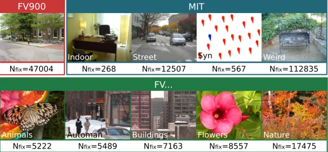
For the study on fixation times developed in Chapter 5 we used three online eye-tracker datasets in addition to the ones depicted in the previous sections. These additional cohorts correspond to ocular recordings from people while free viewing different static images (EHINGER et al., 2009; JUDD et al., 2009; KOOTSTRA; BOER; SCHOMAKER, 2011). The experimental details of each group are described in Table 1. Examples of the visual stimuli of these tasks are depicted in Fig. 8.
FV900 MIT
FV...
Indoor Street Syn Weird
Animals Automan Buildings Flowers Nature
Nfix=47004 Nfix=268 Nfix=12507 Nfix=567 Nfix=112835
Nfix=17475
Nfix=8557
Nfix=7163
Nfix=5489
Nfix=5222
Figure 8 – Stimuli for the online datasets and total number of fixations (Nf ix) in each subgroup.
All datasets can be publicly accessed online following the specifications expressed in the corresponding paper.
Label Reference Equipment # Scenes Subjectsage range # Subjects Visual task
FV900 EHINGER etal., 2009
ISCAN RK-464 video-based eye tracker (240Hz)
912 –
Out-door cities [18-40] 14
MIT JUDD et al.,2009
Information
not
avail-able
1027 – Out-door cities, Indoor, Synthetic, Unclasiffied
[18-35] 15 Free Viewing
FV Animals 12
FVAutoman KOOTSTRA; 12
FVBuildings BOER; Eyelink I 16 [17-32] 31
FV Flowers SCHOMAKER, 20
FV Nature 2011 41
3 Persistence during visual search
The process of eye movement during visual search, consisting of sequences of fixations intercalated by saccades, exhibits distinctive persistent behaviors. In this Chapter we study two different types of persistence present in the scanpaths. Initially, by focusing on saccadic directions and intersaccadic angles, we disclose that the probability distributions of these measures show a clear preference of participants towards a reading-like mechanism (geometrical persistence), whose features and potential advantages for searching/foraging are discussed. We then perform a Multifractal Detrended Fluctuation Analysis (MF-DFA) over the time series of jump magnitudes in the eye trajectory and find that it exhibits a typical multifractal behavior arising from the sequential combination of saccades and fixations. By inspecting the time series composed of only fixational movements, our results reveal instead a monofractal behavior with a Hurst exponent H∼0.7, which indicates the presence of long-range power-law positive correlations (statistical persistence).
3.1 Geometrical persistence
We study the geometrical persistence in eye movement during a visual search task by the analysis of two angles, namely, the horizontal angle, θh, and directional angle,
θd, as shown in Fig. 9. The first refers to the angle between a saccadic event and the
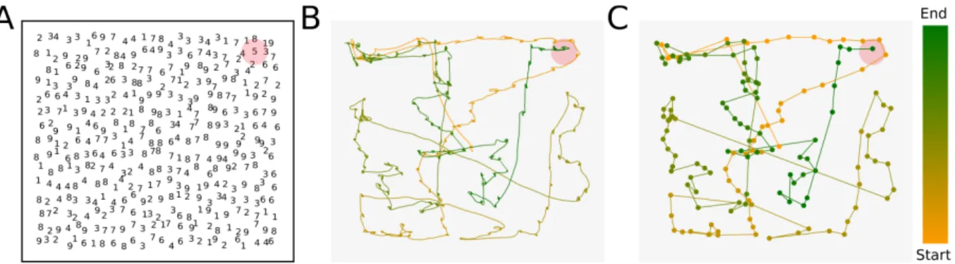
horizontal direction, and the second corresponds to the angle between two consecutive saccadic events. The visual task consists in searching for a unique number “5” embedded in an image of numbers between “1” and “9”, as depicted in Fig. 10A, CN experimental cohort (see Section 2.2.1). In order to study both the horizontal and directional angles we simplify the original trajectories, shown in Fig. 10B, by replacing the fixational and saccadic events by a series of dots and vectors, respectively. As presented in Fig. 10C, the dots correspond to the mean position of a fixation, and the vector between two fixations, i.e. two dots, represents a saccadic event. By doing this we are able to study the persistence in a spatial sense, regardless the time interval of each fixation or saccade. Next, we compute θh andθd. The first one provides information on the anisotropy of the trajectories, whereas
the second provides information on the directional persistence.
The horizontal angle for the i-th saccade is computed as
θhi = arctan(ri,y/ri,x), (3.1)
whereri,x (ri,y) is the x (y) component of vector ri associated with thei-th saccadic event.
The range of θh goes from 0◦ to 360◦ in a counterclockwise sense. For example, if θh is
close to 0◦ it means that the saccadic movement was done with a preference towards the
Figure 9 –Definition of θh and θd. (A) The horizontal angle, θh, refers to the angle
between a saccadic event and the horizontal direction. (B) The directional angle, θd, corresponds to the angle between two consecutive saccadic events.
9 8 8 8 1 1 8 8 6 2 2 9 8 2 3 2 7 2 4 8 9 9 2 3 6 1 8 1 3 2 9 2 4 4 8 1 1 9 7 6 3 1 2 4 9 4 3 8 4 1 6 2 9 1 43 6 9 3 1 8 2 3 8 3 8 6 1 3 3 9 2 2 3 6 9 4 3 4 8 3 4 4 9 1 8 9 9 1 1 3 9 4 8 2 6 7 6 4 3 4 6 7 6 8 7 2 1 8 7 4 7 9 2 3 2 3 2 9 6 7 34 1 4 6 3 8 2 2 6 2 8 7 8 9 76 43 3 1 1 2 4 3 84 4 6 7 6 6 2 2 3 4 8 1 1 8 2 9 4 3 3 1 9 7 4 8 77 8 9 8 7 6 1 7 2 3 2 1 8 7 8 8 9 9 3 7 4 7 6 1 2 9 7 8 88 6 8 92 6 9 8 4 7 3 8 9 3 7 6 3 3 3 7 7 3 4 6 6 6 1 3 7 1 4 4 1 3 11 3 3 3 9 8 2 9 4 8 8 7 43 2 9 6 3 2 1 1 9 1 87 7 7 7 9 3 8 7 3 1 2 93 9 6 4 8 8 8 9 9 9 4 4 98 1 3 4 8 9 9 9 9 8 7 2 3 3 2 1 9 4 2 9 4 9 3 6 7 9 7 7 1 6 2 7 3 3 2 99 2 3 7 83 2 7 1 9 2 3 9 7 9 2 1 3 1 1 4 4 1 4 7 7 3 8 8 3 9 6 6 9 2 2 5 8 4 9 1 6 33 2 9 4 7 2 7 6 3 1 6 8 1 6 6 6 6 3 6 9 9 2 6 7 9
Figure 10 –The experiment. (A) Visual search stimuli. Participants have to search for the unique number 5 embedded in a cloud of numbers between 1 and 9. The red region shows the position of the target, the unique number 5. (B) Eye movement recorded during the experiment. The path going from yellow to green, represents the actual eye trajectory, the color yellow corresponds to the beginning of the search and the green to the ending. (C) Modified eye trajectory. In order to study the eye paths as geometrical entities, we simplified the original trajectory, shown in (B), by reducing the fixations into points and the saccadic events into the vectors between two consecutive fixations, i.e. two points.
that the saccadic movement was done over the horizontal direction from right to left. The inspection of the distribution of θh provides information of the existence of a privileged
direction during the search.
Fig. 11A shows schematically how θh is extracted from an experimental
tra-jectory. As one can see in Fig. 11B, the horizontal angle distribution,P(θh), presents a
clear asymmetry during the visual search. Although the images (Fig. 10A) were prepared in such a way as to prevent any salience and/or directional biases, the subjects prefer to perform a systematic search following a horizontal sweep. This is very different from a regular random walk where the subjects would perform an isotropic search with a uniform distribution forθh, since no direction should be privileged. However, the large percentage
of θh’s falling in the intervals from 315◦ to 45◦ and from 135◦ to 225◦, between 15% and
Figure 11 – The distribution of the horizontal angle (θh) exhibits spatial anisotropy. (A)
Definition of the horizontal angle along the modified visual trajectory, for a real experiment.ri is the vector associated to a saccadic event (red arrows)
as the angleθh denoted in blue corresponds to the angle that goes from the
horizontal direction up tori in a counterclockwise angular direction. (B) The
distribution for θh shows a clear anisotropy in space as the number of counts
is larger for angles associated with thex gaze position. This indicates a search strategy towards a reading-like search.
angle relative to any other direction, rather than the horizontal one, does not change the results. For example, instead of the horizontal angle, one could measure the “vertical angle” and observe the same distribution rotated 90◦.
In order to study the geometrical persistence from one saccadic movement towards the other, we defined the directional angle θd, from 0◦ to 360◦, as
θdi = arctan(r(i+1),y/r(i+1),x)−arctan(ri,y/ri,x). (3.2)
Again,ri corresponds to the saccadic vector at stepi, andri+1 to the one at the subsequent
time step i+ 1. The quantity ri,x (ri,y) denotes the x (y) component ofri from the i-th
saccadic event. From the definition of θd, the movement will be considered persistent if
consecutive saccadic jumps frequently follow a similar direction, namely, if low (close to 0◦) and large (close to 360◦) angle values dominate the distribution
P(θd). Angles with a
value around 180◦ then correspond to anti-persistent movement, that is, a saccadic event
followed by another that goes back in the opposite direction (Fig. 12A). The distribution of θd, as depicted in Fig. 12B, shows a pattern that again differs from the one associated
to a random searcher. If the subject performs a random search with no memory, a uniform distribution P(θd) should be expected. The experimental distribution of θd shows instead
that directional persistence exists along the visual search, having a significant percentage of angles close to 0◦ and 360◦. More precisely, 12% of the angles between saccades are close
500
θd~13°
θd~176°
600 800 1000
800
X[px]
θd~357°
700 900 1100
400 600 800 1000
0 200 400
800 1000 400 600 1100
Y
[p
x
]
A
ri
ri+1
ri
ri+1
ri+1
ri
0.12
0.08
0.04
0.00
P(
θd
)
θd[deg]
0 90 180 270 360
B
Figure 12 – Directional persistence is unveiled by the distribution of the directional angle (θd). (A) Each panel represents a different type of directional persistence.
Different extracts from modified trajectories are presented along with saccade vectorsri,ri+1 (green, red and blue arrows). The directional angle is defined
as the relative angle between both vectors with an angular direction going from ri to ri+1 (small curved arrow). Both ri and ri+1 are drawn into a
coordinate axes to show the angle between them, θd (shaded gray). From
top to bottom: A movement with an almost 13◦ directional angle, showing
counterclockwise persistence; θd close to 180◦ that can be related to a turning
point, or anti-persistent movement, and θd close to 360◦ showing clockwise
persistence. (For better visualization, θd was chosen to be ∼ 13◦ instead of
∼0◦ to show counterclockwise persistence.) (B) The distribution of
θd differs
from a uniform distribution having large peaks at θd ∼ 0◦ and θd ∼ 360◦,
implying that persistence exists during the visual search.
prefer to go on a path following a certain linear direction, at least during a short term. However, there are also some antipersitent movements (i.e. return saccades). This last is shown by the considerable number ofθd around 180◦, representing 5% of all cases.
3.1.1 Reading and non-reading-like search strategies
The previous results suggest that most of the participants prefer to perform a reading-like strategy while looking for the unique number “5”. This could imply that the directional persistence emerges only from those subjects performing these strategies. In other words, if a participant performs a reading like type of search, most of his saccadic movements are done sequentially on the same direction. Therefore, such trajectory exhibits a directional persistence behavior on the horizontal direction.
computed for each trial, we calculate the difference between the count number of angles associated to the horizontal direction and angles associated with the vertical direction. If a trial follows a reading-like type of search then this difference is very large, as there is an anisotropy towards the horizontal direction. On the other hand, this difference diminishes for a trial following a non-reading-like type of search, as there are equal contributions on the horizontal direction as well as on the vertical direction. By setting a threshold (we use a threshold equal to 0.5), we are able to divide our set of trial into two groups:
trajectories that follow a reading-like type of search (81%), and trajectories that follow a non-reading-like type of search (19%).
Trials corresponding to a reading-like strategy exhibit an asymmetry in the distribution, as expected, biased towards the horizontal direction, as shown in Fig. 13A. Those who execute a different strategy have a distribution forθh closer to a uniform one,
as depicted in Fig. 13B, where the preference towards the horizontal direction diminishes. We computed the distribution ofθd values for both groups or search strategies. Fig. 14A
shows that reading-like trajectories exhibit a persistent pattern that is quite similar to the one shown in Fig. 12B for the whole set of trials. Interestingly, for the non reading-like trials directional persistence still appears, as can be seen in Fig. 14B. This reflects that directional persistence exists regardless of the selected strategy, and that θd is a good
indicator of that.
It is also curious how the peak corresponding to antipersistence disappears for the non-reading-like trials. This finding needs to be studied in more detail and may be related to efficiency during visual search. As is generally accepted, in reading tasks the return saccades are used by individuals to facilitate text understanding (BOOTH; WEGER, 2013; SCHOTTER; TRAN; RAYNER, 2014). Such an automatic mechanism could be (consciously or not) used by the participants in our experiment as a way to deal with the problem of information foraging in a visual search context. This can be actually confirmed by studying the correlations between velocity and directional angles (see Figs. 15A and B). For this, we computed the velocity of the previous saccadic movement, defined as Vi =|ri|/∆ti, where ri is the saccade vector corresponding to θid and ∆ti, the duration of
0° 45° 90°
135°
180°
225°
270°
315° 0°
45° 90°
135°
180°
225°
270°
315°
0.00 0.05
0.10 0.15
0.20
0.00 0.05
0.10 0.15
0.20
θ
h[deg]
θ
h[deg]
A
B
Figure 13 –The distribution ofθh shows different strategies for the visual search.(A)Set of
trials that display a reading-like trajectory for visual search. The asymmetry on the number of counts for bins between [315-45]◦ and [135-225]◦ shows
a preference towards a search following the horizontal direction, namely, a reading-like search.(B)Set of trials that perform a type of trajectory different from a reading-like search. The distribution for θh resembles more a uniform
distribution. Although there is a clear asymmetry on the horizontal direction, as well as on the vertical one, it is not as prominent as the one found in (A) .
0.00 0.04 0.08 0.12
0 90 180 270 360
0.00 0.04 0.08 0.12
P(
d
)
d
[deg]
P(
d
)
A
B
0 90 180 270 360
d
[deg]
Figure 14 –The distributions of θd shows different strategies for the visual search. (A)
Distribution ofθdfor the set of trials that follow a reading-like search. Persistent
movements are revealed by the asymmetry in the distribution, with a large number of occurrences with θd∼0◦ and θd∼360◦. (B) The distribution of
θd for the trials that do not show an anisotropic distribution for θh, thus do
not follow a reading-like strategy, also show evidence of persistent behavior on the eye movements. The asymmetry on the distribution of θd, with more
occurrences with θd ∼ 0◦ and θd ∼ 360◦, shows that persistent movements
exist regardless of the strategy employed during the visual task. It is notorious, how the peak related to antipersistence ( θd∼180◦) disappears and is only
0 90 180 270 360 d
[deg]
1.8 2.4 3 3.6 V e lo c it y P re v io u s S a c c a d e [ p x /m s V e lo c it y P re v io u s S a c c a d e [ p x /m s Reading Like0 90 180 270 360
d
[deg]
1.8 2.4 3 3.6
Non Reading Like
A
B
Figure 15 – Saccade velocity profile for the reading and non-reading like trials. Mean
velocity of the previous saccade as a function of θd for trials following a
reading-like trajectory for visual search (A) and for those following a type of trajectory different from a reading-like search (B). Both persistent and anti-persistent saccades carried out by users enrolled on a reading-like strategy are faster than those obtained for other non-reading-like strategies. Thus, this may suggest that an automatic mechanism is at play in the case of reading-like strategies.
3.1.2 Short-range persistence on saccadic events
The distribution of the directional angle shows that there is a directional persistence of the eye paths treated as geometrical entities. In order to study the sequential dependence of the trajectory beyond the pair correlation between consecutive saccades, we study the conditional probabilityP(θi+ℓ
d |θ
[i,i+ℓ−1]
d ) of having a persistence movement at
θid+ℓ given that the previous ℓ−1 movements have also been persistent. Therefore, on a given trial, ℓ is the length of a sequence of persistent saccadic movements starting at the i-th element of the sequence ofθd. For example, imagine that a subject performs a saccadic
movement at θi
d. If ℓ= 2, we compute the probability that θid+2 is a persistent saccadic
movement given that θdi+1 and θi
d also are persistent saccadic movements. Therefore, the
analysis of P provides information on how many saccadic events a participant performs on average within the same relative direction.
We study P for θd in [0:5]◦ or [355:360]◦, which represents saccadic persistent
movements in both counterclockwise and clockwise angular direction. We also study P for θd in [0:10]◦ or [350:360]◦, and θd in [0:20]◦ or [340:360]◦. Analyzing all trials we find