Guilherme José Gago Fial
Bachelor of Computer Science and EngineeringOptimizing Data Selection for Contact Prediction
in Proteins
Dissertation submitted for the degree of
Master of Science in
Computer Science and Engineering
Adviser: Ludwig Krippahl, Assistant Professor, NOVA University of Lisbon
Examination Committee
Chairperson: Jorge Carlos Ferreira Rodrigues da Cruz Raporteur: Daniel Vieira N. Silva Sobral
Optimizing Data Selection for Contact Prediction in Proteins
Copyright © Guilherme José Gago Fial, Faculty of Sciences and Technology, NOVA Uni-versity of Lisbon.
The Faculty of Sciences and Technology and the NOVA University of Lisbon have the right, perpetual and without geographical boundaries, to file and publish this disserta-tion through printed copies reproduced on paper or on digital form, or by any other means known or that may be invented, and to disseminate through scientific reposito-ries and admit its copying and distribution for non-commercial, educational or research purposes, as long as credit is given to the author and editor.
To my friends, family and love. Those that make life worth living.
Ac k n o w l e d g e m e n t s
To begin with, I would like to thank the computer science department (Departamento de Informática) of the University Faculdade de Ciências e Tecnologia da Universidade NOVA de Lisboa for providing me with the opportunity, environment and teachers that allowed me
to learn a great deal about the field of computer science.
I would also like to express my gratitude to my supervisor, Ludwig Krippahl, for introducing me to the interesting fields of bioinformatics and machine learning, and for providing his knowledge and supervision that have guided me through this challenging project. To my colleagues, José Carneiro and Pedro Almeida, for the support with the structure of this final document. To everyone that contributed to this field and developed all the necessary tools, for without them, this work would not have been possible.
Lastly, I would like to thank my family, for their interest and support, particularly my Mother, and to my girlfriend Natalia, for always being there with an endless supply of motivation.
A b s t r a c t
Proteins are essential to life across all organisms. They act as enzymes, antibodies, trans-porters of molecules, structural elements, among other important roles. Their ability to interact with specific molecules in a selective manner, is what makes them important.
Being able to understand their interaction can provide many advantages in fields such as drug design and metabolic engineering. Current methods of predicting protein inter-action attempt to geometrically fit the structures of two proteins together by generating a large amount of potential configurations and then discriminating the correct pose from the remaining ones.
Given the large search space, approaches to reduce the complexity are often employed. Identifying acontactpoint between the pairing proteins is a good constraining factor. If at least one contact can be predicted among a small set of possibilities (e.g. 100), the search space will be significantly reduced.
Using structural and evolutionary information of the interacting proteins, a machine learning predictor can be developed for this task. Such evolutionary measures are com-puted over a substantial amount of homologous sequences, which can be filtered and ordered in many different ways. As a result, a machine learning solution was developed that focused in measuring the effects that differing homolog arrangements can have over the final prediction.
Keywords: Contact prediction, Machine learning, Bioinformatics, Protein-Protein Inter-actions
R e s u m o
As proteínas são uma componente fundamental da vida, atuam como enzimas, anticorpos, transporte molecular, elementos estruturais, entre outros. A capacidade de interagirem de uma forma seletiva com outras moléculas é o que as faz importantes.
Perceber como as proteínas interagem pode trazer benefícios em certas áreas, como a da farmacêutica e a de engenharia metabólica. Os métodos atuais que tentam prever interacções entre proteínas começam por gerar um grande número de encaixes possíveis entre as duas proteínas, de entre os quais se tenta identificar o encaixe correto.
Dado o grande espaço de procura, métodos de redução de complexidade são frequen-temente empregues. A identificação de um ponto de contacto entre as proteínas é um bom factor de restrição. Se pelo menos um contacto for correctamente identificado dentro de um pequeno conjunto de previsões (e.g. 100), o espaço de procura será bastante reduzido.
Para prever contactos, usam-se classificadores juntamente com informação estrutural e evolucionária das proteínas que interagem. No entanto, métodos de informação evoluci-onária extraem essa informação com base num grande número de sequências de proteínas homólogas, as quais podem ser filtradas e ordenadas de diferentes maneiras. Após de-senvolver classificadores de contactos, a tese foca-se em medir os efeitos de diferentes configurações de homólogos.
Palavras-chave: Proteína, Previsão de Contactos, Aprendizagem Automática, Bioinfor-mática
C o n t e n t s
List of Figures xvii
List of Tables xix
Listings xxi Glossary xxiii Acronyms xxv 1 Introduction 1 1.1 Motivation . . . 1 1.2 Objectives . . . 2 1.3 The Protein . . . 3 1.3.1 Amino Acids . . . 3 1.3.2 Structure . . . 4 1.4 Protein Docking . . . 5 1.4.1 Docking stages. . . 6
1.4.2 Improving the Docking . . . 7
1.5 Information for contact prediction . . . 7
1.5.1 Evolutionary information . . . 7
1.5.2 Structural and physicochemical information. . . 9
1.6 Summary . . . 11
2 State of the art 13 2.1 Evolutionary information. . . 13
2.1.1 Protein Sequence Comparison . . . 13
2.1.2 Conserved residues . . . 15 2.1.3 Coevolved residues . . . 16 2.2 Structural characteristics . . . 16 2.2.1 Solvent accessibility. . . 16 2.2.2 Secondary Structure . . . 17 2.3 Physicochemical characteristics . . . 17 2.3.1 Hydrophobicity . . . 17
C O N T E N T S
2.4 Machine Learning . . . 18
2.4.1 Decision Trees . . . 18
2.4.2 Support Vector Machines. . . 21
2.4.3 Neural Networks . . . 22
2.4.4 Logistic Regression . . . 23
2.4.5 Naïve Bayes Classifier (NBC) . . . 24
2.5 Evaluation . . . 25
2.5.1 Cross-Validation . . . 26
2.5.2 Measurement of classifier performance. . . 26
2.6 Data . . . 28
2.6.1 Protein Data Bank. . . 28
2.6.2 Data Extraction . . . 28
2.7 Comparable methods . . . 29
2.7.1 Coevolutionary-derived contact predictors. . . 29
2.7.2 Machine learning-based contact predictors . . . 30
3 Development 31 3.1 Tools . . . 31
3.2 Data Preparation. . . 32
3.2.1 Homolog Extraction. . . 32
3.2.2 Preparing the homologs . . . 35
3.3 Feature Preparation . . . 40
3.3.1 Preparatory Steps . . . 41
3.3.2 Feature Extraction. . . 43
3.3.3 Post Processing . . . 44
3.4 Model Building . . . 48
3.4.1 Model & Hyperparameter optimization . . . 48
3.4.2 Final Model . . . 52
4 Results and Discussion 53 4.1 Homolog Similarity Comparison. . . 54
4.1.1 Homolog percent identity . . . 54
4.1.2 Homolog percent similarity . . . 56
4.2 Homolog Order Comparison . . . 57
4.2.1 Ordering by a similarity measure . . . 57
4.2.2 Ordering by cluster . . . 58
4.3 Homolog Quantitative Comparison . . . 58
4.4 Discussion and Test Results . . . 60
4.4.1 Test on the improved configuration . . . 60
4.4.2 Test on the baseline . . . 61
4.4.3 Feature importance . . . 62
C O N T E N T S
5 Conclusion and Future Work 63
Bibliography 65
L i s t o f F i g u r e s
1.1 Anatomy of an amino acid [Bur08]. . . 3
1.2 The four levels of protein structure [Bra+99]. . . 5
1.3 MSA of 5 hemoglobin proteins (Generated under the UniProt website using Clustal Omega). . . 8
2.1 A pairwise alignment between two sequences. . . 14
2.2 For a two class problem, the thick line defines the boundary and the dotted lines the limit of the margin on both sides. The dot and plus signs represent the classes, the ones encircled are the support vectors [Alp10]. . . 21
2.3 Sigmoid activation function. . . 24
3.1 Unordered and unpaired homologs. . . 38
3.2 Ordered and paired homologs. . . 38
3.3 Unordered and unpaired homologs. . . 39
3.4 Ordered and paired homologs. . . 40
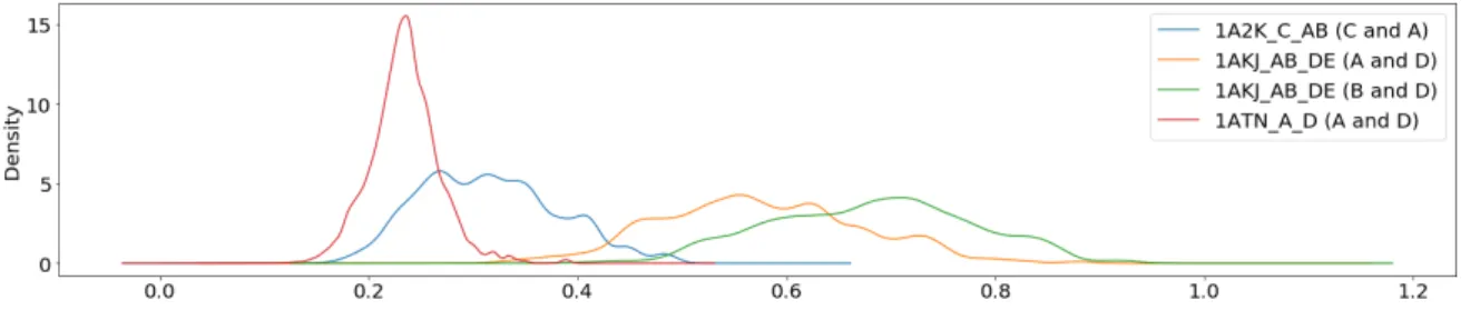
3.5 Distribution of co-evolutionary values across different complexes before scaler. 46 3.6 Distribution of co-evolutionary values across different complexes after scaler. 47 3.7 Complex 4JCV, how the ABCD chains from one partner connect to chain E from the opposing partner. . . 47
4.1 Comparison of different percent identity configurations. . . 55
4.2 Comparison of different percent similarity configurations. . . 57
4.3 Performance comparison between randomly ordered homologs and identity ordered homologs. . . 58
4.4 Performance comparison between identity ordered homologs and first cluster constrained ordered homologs. . . 59
4.5 Performance comparison by using different limits. . . 59
4.6 Feature importance for Logistic Regression and Random Forest for classifying in the tuned data. . . 62
L i s t o f Ta b l e s
3.1 Benchmark 5.0 entries . . . 33
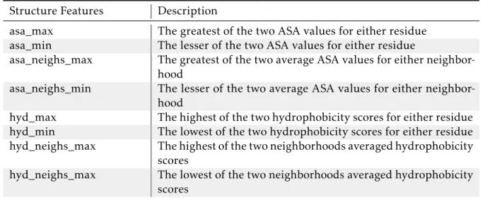
3.2 Overview of structural features . . . 44
3.3 Overview of homology features . . . 45
4.1 Number of available complexes for several identity thresholds. . . 54
4.2 Number of available complexes for several percent similarity thresholds. . . 56
4.3 Comparison between testing with restricted data and unrestricted data, us-ing quantiles, mean and percentage of complexes havus-ing at least one correct contact in the given top positions. . . 61
G l o s s a r y
contact Residue-residue contacts, inter-contacts, or simply contacts, are pairs of residues that belong to different proteins, and have a distance no longer than 5Å.
docking Docking is a computational procedure that seeks to find the position and orientation between two molecules.
hyperparameters Necessary parameters that control how a machine learning model learns from the data.
Ac r o n y m s
C
h
a
p
t
e
r
1
I n t r o d u c t i o n
In this chapter, the overall motivation and objective of this work will be provided, as well as the necessary biochemical background concepts such as the protein and its structure, protein dockingand the attributes within proteins that facilitate the intendedcontact
prediction.
1.1
Motivation
Proteins are essential to life across all organisms. They are responsible for most of the work within the cell by regulating its processes and enabling signals to be imported and exported into and out of the cell. They also act as enzymes that catalyze chemical reac-tions, transporters for small molecules, antibodies, messengers (hormones) and structural components that provide movement, structure and support [Bur08;Pro].
The biological function of the protein depends on its 3-dimensional structure and how it connects to other structures and proteins, not simply on the sequence of building blocks that compose it [Bra+99]. It is therefore fundamental to understand how proteins interact and what is the assembled structure they form, designated a protein complex. Such knowledge would grant scientific advantages in areas like drug design or metabolic engineering. As an example, anti-retro-viral drugs supply molecules that bind to the viruses’ reverse transcriptase and block its ability to convert viral RNA to DNA, stopping the viruses’ replication capability.
Current practical methods for determining protein structures, such as X-Ray crystal-lography, are complex and lengthy laboratory processes, with an increase in difficulty depending on the size of the protein. For this reason, despite having resolved structures of individual constituent proteins, the complexes they form are often unknown. As a re-sult, methods that attempt to computationally solve this problem were developed, known
C H A P T E R 1 . I N T R O D U C T I O N
as protein docking.
In the most general form, the docking algorithms attempt to geometrically fit the two protein molecules together. However, doing so with no additional information leads to an overwhelming number of potential conformations to be tested, among which, only a select few correspond to a native pose, as found in the actual complex.
It is computationally unfeasible to thoroughly test each potential pose, and so there is a critical need to filter out bad conformations. Typically, this is done by applying fast filtering functions which reject likely wrong conformations. However, the small number of native poses might still end up being filtered out and the docking will produce no correct results.
One way of filtering would be to develop a prediction mechanism that would issue a set of possible contacting points between the two interacting proteins, ideally guaran-teeing at least one correct prediction within the set. From here, conformations can be restricted to those including one of the predicted contact points.
Besides using structural and chemical features, an interesting way of possibly deter-mining the location of such contact points is to look at evolution. That is, by analyzing homologous proteins that carry the same function across different organisms, one can de-termine evolutionarily conserved or co-evolved points, which can be indicative of contact locations.
1.2
Objectives
The motivation requests the development of a protein-protein contact predictor by using machine learning and features extracted from the constituent proteins’ three-dimensional structures and homologous protein sequences.
The homolog protein data is the basis for the extraction of evolutive information, as a result, practical questions were raised relative to the collection and organization of the homolog protein data, and how it affects contact prediction.
For this reason, the optimization of the homolog data selection and a measurement of its contribution are the goal of this thesis. Thus, while there is a variety of structure based attributes that are certainly helpful for contact prediction, the focus is on information that can be extracted from the homolog sequences.
Therefore, different ways of arranging the homolog data were devised and predictions were made under different setups in order to draw a conclusion regarding an ideal data preparation. To determine the predictive success, the protein docking benchmark dataset (DBMK 5.0) is used. It provides known complex structures. This way, predicted contacts are compared to the actual contacts in the structure.
1 . 3 . T H E P R O T E I N
1.3
The Protein
Proteins are molecules present in every living system, their capability of interacting with specific molecules in a very selective manner, including other proteins, makes them essential in most biological processes.
In this subsection we will provide an overview of the structure of the protein, namely the structural properties relevant to our goal of contact prediction.
1.3.1 Amino Acids
Proteins are essentially a chain of amino acids (or residues, when an amino-acid is in-corporated into a chain, water is released, turning into an amino-acid residue, or simply residue) linked together by peptide bonds: a polypeptide chain, where the amino-acid is the building block.
Amino-acids consist of a central carbon (Cα), which connects to an hydrogen atom (H), a
carboxyl group (COOH), an amino group (NH2) and a sidechain, denoted by the letter R,
as depicted in figure1.1.
The sidechain sets difference between the 20 distinct amino-acids that can be found
Figure 1.1: Anatomy of an amino acid [Bur08].
on most living systems. These sidechain differences manifest themselves as particular attributes per amino-acid, chemical functionality and structure vary from one to another, however, they are grouped by similar attributes [Gro10].
In this regard, we can arrange them into four main categories: non-polar hydrophobic, polar-uncharged, polar-charged positive and polar-charged negative. These properties can provide an insight about the structure and fold of the protein and possibly how it might bind to other molecules. For instance, hydrophobicity has been demonstrated to affect structural properties. Hydrophobic residues can usually be found on the hydropho-bic core of the protein, or in contact with one another when in aqueous environment, due to their water repulsive properties. Hydrophilic residues may in turn remain in contact with water [Bur08].
C H A P T E R 1 . I N T R O D U C T I O N
1.3.2 Structure
The chains of amino-acids that constitute a protein can assume lengths spanning from as few as 20 to more than 5000 residues. In order to be able to portray them, there are four structural description levels. Namely Primary, Secondary, Tertiary and Quaternary (figure1.2).
Primary Structure The first level, denoted as primary structure, is simply a list of the composing amino-acids in their order of appearance, analogously to reading the protein chain from one end to another. Their spatial distribution is not described.
Secondary Structure The secondary structure is a description of the spatial arrange-ments of amino-acids in the peptide chain induced by hydrogen bonds. Specifically, these arrangements cause the chain to form a particular recurrent shape, it is this shape that is described and not the physical positioning of the residues in the tridimensional space. Commonly, the secondary structure is categorized by one of three shapes: α-helices, β-strands and loops [Bur08].
The alpha helix takes place when the backbone of the chain winds in a helical conforma-tion around the long axis of the molecule with the R groups of the amino-acids facing outward from the helix. This coil pattern develops due to the hydrogen bond that the residue n has with the residue n + 4 ahead in the chain. As a result each turn in the helix is composed of 3.6 residues, however, there are other infrequent forms that allow more elongated helices, like the 310helix with 3 residues per turn that is usually found at the
end of alpha helices, or the more uncommon pi helix with 4.4 residues per turn [Bur08]. A beta strand is a strip of the polypeptide chain that is almost stretched in a line. When several beta strands are parallel to each other and connected by hydrogen bonds between their carboxyl oxygens and their amide hydrogens, they form a beta sheet, where this sheet forms a plane-like structure (which may be twisted). When all connected strands rise and fall together, we have a beta-pleated sheet. Additionally, the beta strands can be classified as parallel or anti-parallel. If the strands have the same orientation, i.e. the amino acid indices on the parallel strands increase in the same direction, it is a parallel beta strand. Otherwise, it is labeled as anti-parallel [Bur08;Gro10].
The Loop, or omega (Ω-) loop, is categorized as a non-regular secondary structure, unlike the α-helix and β-strand. This is due to not having repeating hydrogen bonding patterns. The loops are characterized by the loop-like three-dimensional form contracted by the polypeptide chain, usually having the beginning and end residues of the loop proximal in space. Furthermore, they often connect other secondary structures and are in great part found on the surface. The loops have been found to be regularly involved in protein function and molecular recognition [Fet95], most likely as a result of their flexibility and surface availability, along with pattern free arrangement unlike regular structures. The secondary structure of a residue may contribute to the likelihood of it being a contact.
1 . 4 . P R O T E I N D O C K I N G
For instance, it has been observed that contact residues appear to be more frequently part of a loop formation [OR07].
Tertiary Structure The tertiary structure allows the full visualization of a protein in three-dimensional space. Strictly speaking, it provides the full three-dimensional struc-ture of the polypeptide chain with atomic detail. The interactions of residues that are far apart in the primary structure are represented here, mainly through non-covalent interactions, thus allowing the depiction of the positional relationships of the secondary structures [Bur08].
Quaternary Structure Lastly, in the same fashion, the quaternary structure is the spa-tial relationship of multiple tertiary structures that are grouped together, forming an oligomeric complex. Therefore, an oligomeric complex, or protein complex, is an assem-bly of several polypeptide chains. In other words, two or more proteins linked together by non-covalent bonds.
The surface area enclosed by two given proteins that are forming a complex is termed interface. However, in the interface only a small subset of residues is actually essential for the binding between the two protein partners, they are commonly referred to as hotspots, or contacts.
The aim of this work is therefore aiding the prediction of protein complexes [Bur08]. How the complex prediction is attempted and how contact residue prediction will assist is covered in the following section.
Figure 1.2: The four levels of protein structure [Bra+99].
1.4
Protein Docking
Docking is a computational procedure that seeks to find the best matching configuration between two molecules, designated receptor and ligand, in pursuit of predicting the bound molecule complex resulting from their association [Hal+02], therefore making protein docking the prediction of a bound protein-protein complex given two known protein structures (protein targets)[KB15]. These protein structures naturally have to be experimentally extracted and determined, and it can be done two ways. Either we derive the structure from a complexed state, that is, while it is coupled to any other molecule, or
C H A P T E R 1 . I N T R O D U C T I O N
when it is free in solution in an uncomplexed state (native structure). Consequently, the docking can then be attempted using bound or unbound molecules. The bound docking, the simplest, seeks to dock a receptor and a ligand considering the same shape they have when found connected to one another, disregarding the natural conformational changes that occur when they are separated, this is not realistic. The docking will be most useful when attempting to couple uncomplexed structures, as these are what we have at our disposal when the structure of the complex is unknown. Therefore, efforts should be focused on the unbound docking. Such docking works with molecular structures that may be uncomplexed (native structure), or bound to other molecule other than the one that is being attempted to dock with (pseudo-native structure), or even modeled ones [Hal+02].
In short, the docking problem can be described as follows: "Given the coordinates of two molecules, predict their correct bound association", as stated in [Hal+02].
1.4.1 Docking stages
Computing the docking can be a very expensive task, especially if attempted in its most basic form where we have no additional information other than the structure of the two molecules. This is due to the fact that there is a great number of ways of placing two molecules together while considering three levels of rotational and translational freedom. To illustrate, combining every residue on the surface of a protein with all the surface residues on the other could easily yield a number in the order of 107possible combinations [Hal+02]. The difficulty rises further when taking into account the unbound state and the flexibility of the molecular structures, since each molecule can now pose in several different conformations.
The docking procedure divides the problem in two stages: the searching (or filtering) and the scoring stage [Hal+02].
Search/Filtering stage: With the current computational capabilities, it is unfeasible to perform a thorough evaluation (scoring) of all the possible molecular arrangements in order to sort out the best. To tackle this, a search stage is employed.
At this stage, the goal is to retain a subset of most likely correct molecule configurations from the large sample of possible molecular arrangements. To do so, fast and coarse functions are applied over the search space to weed out incorrect conformations all the while keeping the correct solutions [Hal+02].
The subset of filtered candidates is then passed onto the next stage.
Scoring stage: The goal of the scoring stage is to identify the correct or near-native conformations within the reduced set of candidates provided by the search phase. Through the use of heavier and more complete functions that implement strategies like
1 . 5 . I N F O R M AT I O N F O R C O N TAC T P R E D I C T I O N
energy minimization, each candidate is evaluated more in depth and attributed a rank. Ideally, the top ranked solutions would correspond to the correct models [Hal+02;KB15].
1.4.2 Improving the Docking
One way of improving the docking results would be to improve the scoring phase, in which case the scoring functions would then rank the correct conformations more accu-rately. Another way would be to improve the searching phase, which in turn provides more suitable candidates for the scoring phase.
While scoring is important, if the searching fails to select any correct conformations, then a correct model can never be found irrespective of how good the scoring functions are. It is in this filtering stage that contact prediction may prove to be a useful addition. The locations of possible contacts between the two protein partners can be used as a constraint when picking a set of candidate conformations to pass onto the scoring phase. Even if there is only one correct contact among all the predicted contacts, then we can already increase the fraction of correct docking configurations in the set of candidate models [KB15].
1.5
Information for contact prediction
For distinguishing contacting from non-contacting residues, information is needed. The contacts between proteins happen by virtue of some form of compatibility. If we wish to predict such contacts, attributes that may lead to understanding this compatibility must be gathered and tested with machine learning in pursuit of bettering predictive capabilities.
The following aspects were deemed relevant for feature extraction regarding the predic-tion of protein-protein contact points.
1.5.1 Evolutionary information
All living beings have relatives and ancestors as a result of evolution, and so do the proteins within them. Proteins from different organisms that carry out the same function are usually similar, in this sense, if two proteins share ancestry between them, they are called homologous. Such homologs often share significant sequence identity, that is, a certain percentage of amino acids in their sequence are observed in the same sequential order.
Since contact residues are essential participants on maintaining and establishing the interaction between two proteins, and considering that the resulting protein may lose functionality or structure upon the loss of a contact, throughout evolution such residues tend to be conserved or correlatively mutated in order to maintain such contact points. In such a way, by analyzing several homologous sequences, insight on which residues have been mutated or conserved across protein relatives can be obtained. Such information
C H A P T E R 1 . I N T R O D U C T I O N
helps to pinpoint some potential contact locations on the target protein [MG08].
Additionally, evolutionary methods allow for a more universal and wide applicability due to conservation patterns being more easily recognizable across different functional sites, where physicochemical properties may vary [AA+15]. Hence, evolutionary data already proved useful for several contact, binding site and interface predictors [Gon+13;KB15;
OR07].
1.5.1.1 Sequence alignments
The first step towards extracting useful information from several homolog sequences is to carry out a Multiple Sequence Alignment (MSA). The rationale behind MSA is to, ideally, align multiple homolog sequences in a way that equivalent residues in terms of structure and functionality end up aligned in a one-to-one correspondence across all sequences, with positions that are unable to align being represented by a (-) symbol, called gap [Rus14] (figure1.3illustrates an alignment).
Figure 1.3: MSA of 5 hemoglobin proteins (Generated under the UniProt website using Clustal Omega).
The MSA is the multiple sequence counterpart of a Pairwise Alignment, where only two sequences are aligned.
1.5.1.2 Conserved amino acids
As briefly revealed in the introduction of this section, conservation can be indicative of a possible interaction residue. The logic behind it is that these contact residues are crucial to the whole function of the protein since they mediate the interactions directly, thus having a considerable impact if disrupted. Having taken this into consideration, such residues will likely be under evolutionary pressure against mutation, therefore being identifiable by their conservation across homologs [AA+15].
1.5.1.3 Coevolved amino acids
Residue conservation has had conflicting views regarding hotspot prediction. Some stud-ies have found interacting residues not to be highly differentially conserved in comparison to the rest of the protein, or that their use brings little predictive improvement, while some other studies indeed found conservation to be greater among interface residues, where several methods based solely on conservation delivered significant results. Perhaps such a difference may originate from different datasets and methods [AA+15]. Irrespective of its significance, conservation does not provide mutual information between two interacting
1 . 5 . I N F O R M AT I O N F O R C O N TAC T P R E D I C T I O N
partners, that is, given several conserved residues on one protein and several on the other, no clue is provided from the conservation alone about which pairs of conserved residues are potential contacts [MG08]. To this end, coevolution allows the inferring of potential contacting residues. The rationale is the following: different organisms can have homol-ogous proteins, however, they often differ in amino acid composition, having different amino acids in certain positions [Ovc+14]. By comparing protein complexes existing in different organisms, it can be deduced which amino acids change in both protein partners in a compensatory way, leading to the uncovering of potential contacting residues, since a mutation in one side must often be accompanied by a compensatory mutation on the other side to maintain compatibility [KB15].
1.5.2 Structural and physicochemical information
In the previous subsection, it was explained how evolutionary insights allow us to deduce which residues might be part of protein-protein interactions.
In this subsection, residue structural and physicochemical attributes will be presented. Such properties will help further constrain the possibilities when evaluating potential contacts.
1.5.2.1 Solvent Accessibility
Solvent accessibility is often chosen as one of the most discriminatory structural features for interface and hotspot related predictions [AA+15]. The solvent-accessible surface area depicts how exposed to the solvent is a given area. No exposition to the solvent means that the aforementioned area is buried within the molecule and thus cannot be accessed on the surface, indicating its unlikeliness on making part of a protein-protein interaction, since these interactions take place upon the reachable surface. Solvent accessibility has been shown to be higher in inter-protein contact residues [OR07], when in an uncomplexed state. However, this does not always seem to be true. The O-Ring theory states that contact residues are usually located at the center of a particular interface area and surrounded by energetically less important residues that shape like an O-ring to occlude bulk water molecules from the contact residue [LL09]. Though this is applied over a bigger patch of surface, it has inspired the use of both the residue and its surrounding nearby residues accessibilities as features.
1.5.2.2 Hydrophobicity
Hydrophobicity has proven to be of great value to the prediction of protein interactions, there is an evident overall tendency of hydrophobic residues to interact with each other, as they constitute the most common residue pairing. Moreover, hydrophobic-hydrophilic residue pairings were associated low contact values as well [Gla+01].
Additionally, the hydrophobicity of neighboring residues might be of relevance consider-ing their evident proximity to the residue at hand. That is, in an actual contact, the surface
C H A P T E R 1 . I N T R O D U C T I O N
neighborhoods of either contacting residue are likely to be proximally close and should have some form of complementarity. Therefore, both the hydrophobicity of residues and their neighbors constitute interesting properties to help determine the feasibility of a potential contact.
The following amino acids are hydrophobic [BR03]:
• Very hydrophobic: Valine, Isoleucine, Leucine, Methionine, Phenylalanine, Trypto-phan and Cysteine.
• Less hydrophobic (or indifferent): Alanine, Tyrosine, Histidine, Threonine, Serine, Proline and Glycine.
• Part hydrophobic (i.e. the part of the side-chain nearest to the main-chain): Arginine and Lysine.
1.5.2.3 Other attributes
Other residue attributes were initially considered and implemented, such as residue type, secondary structure and charge. However, they were eventually left out as the objective shifted to analyze the impact of different homolog data arrangements. Different arrange-ments merely impact evolutionary features, thus, optimizing the contact detection by means of further structural and physicochemical features is suitable for future work. The research and rationale of choice for such features can be found under this section.
Residue type The amino acids differ from each other and have different representations when considering hotspot residue composition. It has been reported that the fundamental hotspot forming residues are tryptophan, arginine, and tyrosine, composing 21%, 13.3% and 12.3 % of hotspots found in interfaces, respectively. On the other hand, other types such as leucine, serine, threonine and valine, seem to be underrepresented as hotspots [Mor+07].
Secondary Structure It has been shown that the secondary structures to which the amino acids belong to are not equally represented in hotspots. In addition, their distri-bution was found to vary between hotspot interface residues and non-hotspot residues by [OR07; Wan+12], having 57% of hotspot residues belonging to a loop structure. A possible explanation being that loops are somewhat more flexible and might constitute good contact points. To this end, it is interesting to use the type of secondary structure associated to a given residue as an additional attribute that might help pointing out a most likely hotspot residue.
Charge Certain residues have either a negative or a positive charge, given that opposite charges attract each other and that same charges repulse one another, such properties
1 . 6 . S U M M A RY
may help determine the likeliness of two given residues forming a contact. Oppositely charged residues have demonstrated a tendency to be in contact with each other while negatively charged residues displayed a low contact propensity. However, there was an average pairing tendency among positively charged residues, e.g. arginine and lysine. In this particular case, the arginine and lysine had a specific orientation so that their charged amino groups would be as far as possible from each other, seemingly to minimize the repulsion between them. They appear to constitute a pair due their solvent accessibility and close packing attributed to hydrophobic interactions, which diminish their mutual repulsion.
Additionally, there was a favorable connection between hydrophobic and charged residues [Gla+01], advocating for an interplay of both physicochemical attributes.
1.6
Summary
To summarize, the objective is to develop a contact predictor based on structural and evolutionary information, with a focus on the latter, and then test for differences in the predictive quality depending on the protein homolog arrangement, which is the basis for deriving evolutionary information.
To ready homolog protein data such that any evolutionary based attributes can be computed, the homologs of each protein must be aligned, as explained in detail above at 1.5.1.1. From these alignments, conservation and co-evolutive attributes are then computed.
For conservation (1.5.1.2), each residue in the protein is attributed a value describing how conserved it is across the homologs, it is therefore dependent on the quality of the available homologs for that protein, and the alignment produced.
For co-evolution (1.5.1.3), a value is attributed for each pair of residues between two connecting proteins, which is dependent on the homolog alignments of both proteins and which homologs from either protein are assumed to connect with each other. Thus being subject to not only the homolog quality, but the order between the two sets of homologs. From the protein structure, the solvent accessibility (1.5.2.1) is computed for each residue. It is undoubtedly a good structural descriptor for this problem, as most contact residues are on the surface of the proteins, and can therefore rule out residues that are too buried into the protein. As discussed earlier, more structural attributes could be used, but those would not be affected by the homolog configurations.
Another attribute is hydrophobicity (1.5.2.2), residues are given a value representing how hydrophobic they are. This information can be used in conjunction with the ho-molog alignments, providing descriptors such as the average hydrophobicity across the homologs for a particular residue.
Multiple features are then computed based on this information. This is explained in detail during the development chapter, in the feature extraction section at3.3.2.
C
h
a
p
t
e
r
2
S ta t e o f t h e a rt
In the introduction, several important concepts necessary for understanding this project were presented. A brief description of the techniques used to implement such concepts along with a comparison among different state-of-the-art implementations is provided in this chapter. In the first three sections, the specialized software and techniques required for extracting information from evolutionary, structural and physicochemical is discussed. Following, common machine learning methodologies are introduced that were initially considered for use. Afterwards, it is explained how to evaluate the prediction results on this particular problem, where and why the data is obtained from and lastly, other relevant contact prediction related methods are discussed.
2.1
Evolutionary information
In this section, the necessary methodology for the extraction of evolutionary information is described and analyzed.
2.1.1 Protein Sequence Comparison
Comparing protein sequences is the base procedure upon which homology can be in-ferred, and homology is the basis for extrapolating any kind of evolutionary information. This subsection will present the principal mechanisms with which sequences are compared.
2.1.1.1 Pairwise Sequence Alignment
In order to be able to measure how identical two protein sequences may be, a two se-quence alignment must be performed, termed the Pairwise Alignment. From such an alignment a score is then deduced that quantifies their similarity.
C H A P T E R 2 . S TAT E O F T H E A R T
The two standard scores for analyzing the similarity between two sequences are the percent identity and percent similarity [Pea13], and the two types of alignment that can be performed are the global and the local alignment [Rus14].
Figure 2.1: A pairwise alignment between two sequences.
Global and local alignments
There are two main approaches to sequence alignment, the global and the local alignment. The global alignment takes the entire sequences into account, that is, it seeks to match the sequences end to end with the highest possible score, it is best used when the sequences are of similar lengths and homologous. On the other hand, the local alignment aims at matching parts of the sequences without being forced to align them entirely, such an approach is more suitable for the discovery of conserved domains, or to align sequences significantly different in length.
In this work, the conservation and coevolution of residues is to be explored by aligning protein homologs that should interact in the same way, as such, global alignment is assumed to be the most suitable method [Rus14]. It is presumed that such proteins should be globally similar.
Similarity scores
After two sequences are aligned, residue with residue, we can evaluate the alignment with percent identity or percent similarity, the differences are explained below.
The percent identity uses an identity matrix that simply attributes 1 to identical residue pairs and 0 to all other pairs. This essentially results in counting the matching residues on the alignment that have the same amino-acid (perfect match) and dividing the result by the length of either the smaller or larger sequence to obtain a percentage. If divided by the smallest length, it will essentially rate how well does the smaller sequence match with any sub-part of the bigger sequence (e.g. sequence ABBACA and ABBA are 100% similar), this is suitable to rank local alignments. Contrarily, if divided by the bigger length, the extremity gaps and size differences matter, which is more suitable for the situation where one intends to find homolog sequences and not just fragments or regions, that is, a global alignment (e.g. ABBACA and ABBA are now 67% similar).
Percent similarity follows the same strategy as percent identity explained above, ex-cept that it uses a substitution matrix rather than an identity one.
In short, substitution matrices are matrices that quantify the interchangeability be-tween any two residue types, that is, residues that often replace one another when ana-lyzing mutations between homologous sequences. If any two residues map to a positive
2 . 1 . E V O LU T I O N A RY I N F O R M AT I O N
value, they have been observed to replace one another whenever mutations occur in ho-mologous sequences, if they map to a negative value instead, they have been observed to avoid being replaced by one another.
Hence, by using a substitution matrix, a value of 1 will be attributed whenever the aligned residue pair has a positive number, otherwise, 0 will be attributed.
Among substitution matrices, the most common ones are PAM (Point Accepted Muta-tion) [Day+78] and BLOSUM (Blocks Substitution Matrix) [HH92].
To summarize, percent identity has a very strict matching mechanism, where only the exact same residues are accepted as a match. Well rated sequences regarding identity are indeed very similar. Once homology has been established, it is a reasonable similarity score [Pea13].
On the other hand, in contrast with identity, percent similarity has a more relaxed matching mechanism, since it accepts residue pairs on the alignment that have been observed to substitute each other according to any given substitution matrix. Well rated sequences with this approach are not necessarily well rated on identity.
The standard algorithms for implementing local and global alignments are the Smith-Waterman and Needleman-wunsch algorithms [NW70], respectfully.
The pairwise2 module of the Biopython package [Coc+09] already implements the alignment algorithms.
2.1.1.2 Multiple Sequence Alignment
As briefed over the introduction under1.5.1.1, the Multiple Sequence Alignment (MSA) procedure aligns three or more protein sequences with assumed evolutionary relationship and is the preceding step required to be able to discern evolutionary characteristics such as the conservation and coevolution of residues.
The most common algorithms used for global multiple sequence alignments have been the Clustal algorithms. The T-Coffee algorithms are also fairly popular due to their increased accuracy [SH14]. In this work the latest version of the Clustal algorithms, Clustal Omega, will be used for the alignments. The reason for choosing Clustal over T-Coffee, at least initially, is that the T-Coffee increased accuracy of 5-10% comes at the expense of performance, usually being limited to a few hundred sequences. Oppositely, Clustal Omega allows for sizable alignments (190,000 sequences took a few hours on a single processor) while maintaining accurate results. Furthermore, Clustal Omega revealed through benchmarking tests to be more accurate than most of the frequently used fast methods and still comparable to some of the slow intensive methods [Sie+11].
2.1.2 Conserved residues
The two most recognized tools for calculating evolutionary conservation at each site of a given MSA are AL2CO [PG01] and Rate4Site [Pup+02][AA+15;CP09].
C H A P T E R 2 . S TAT E O F T H E A R T
The choice is Rate4Site since it is reportedly more accurate than previous methods [May+04], among the best for large alignments with more than 50 sequences [JT10] and it has been consistently used in research related to contact and hot-spot prediction [AA+15;
Ezk+09;MG08;Tun+09].
The computed scores are a relative measure of evolutionary conservation, a low value indicates that the position in the MSA is most conserved.
2.1.3 Coevolved residues
In the coevolution approach, residue positions within a MSA are analyzed for correlated changes as a sign of coevolution and therefore direct residue contact. One issue is that residues might coevolve indirectly, i.e. if residue A is coupled to residue B and B to a residue C, then one may falsely conclude that A is in contact with C [Kam+13]. To tackle this, recent methods such as Direct Coupling Analysis (DCA) [Mor+11] and PSICOV [Jon+12] used an inverted residue-residue covariance matrix technique to accomplish the separation of indirectly and directly coevolved residues [Kam+13]. However, more recently, methods such as GREMLIN [Kam+13] and plmDCA [Eke+13] have achieved higher accuracy with a different approach (Pseudo-Likelihood Maximization) [Kam+13;
See+14]. CCMPred [See+14] is an efficient open-source implementation of these top
performing approaches and will be the chosen software for this task[See+14].
CCMPred calculates direct coevolution strength between any two residues of a MSA [Zho+17], as it is designed to predict intra-contact residues to help fold prediction. To measure the coevolutive strength between two partner proteins of a complex, both MSA’s belonging to each one must be concatenated, linking sequences belonging to the same species (same complex), creating a paired sequence alignment. The paired alignment will then be fed into CCMPred to reveal direct coevolving residues within the complex, where only residue pairs (potential contacts) that are on the surface and belong to both partners are to be considered.
2.2
Structural characteristics
2.2.1 Solvent accessibility
Solvent accessibility, or Accessible Surface Area (ASA), is calculated based on an algorithm which simulates a probe rolling around the Van der Waal’s surface of the molecule [LR71;
SR73]. The probe is typically given the radius size of water (1.4 Å), which is the solvent, and then rolled over the 3-dimensional coordinate structure of the protein. The path traced out by the center of the probe defines the accessible area [HN93;LR71;SR73].
There are several tools to calculate ASA values [Cav+03; HN93; Mih+08; Mit16;
Tou+15], however, they generally follow the same algorithm and therefore output similar values, the main differences lay in usability, format and calculation speed.
2 . 3 . P H Y S I C O C H E M I C A L C H A R AC T E R I S T I C S
DSSP was initially considered, as it is a standard database/tool to use with PDB entries which provides secondary structure and accessibility information [Tou+15]. However, the structure files extracted from DBMK sometimes had non-standard residues which caused DSSP to ignore them and possibly not account for their interference with neighboring residues.
As a result, a python library that provides utility functions to analyze PDB structures was used to calculate the ASA values [Ho18].
2.2.2 Secondary Structure
To determine the secondary structures within a given protein structure, the de facto
standard is the DSSP (Dictionary of Protein Secondary Structure) software and databank [KS83; Tou+15]. Essentially, the DSSP software determines the secondary structures and calculates other structural properties from the PDB entries and places them on the equally named databank [Tou+15]. DSSP does not predict the secondary structure, it assigns it based on hydrogen bonding patterns [KS83].
In a study published in 2005, the authors of SEGNO [Cub+05] compared it to DSSP and STRIDE [HF04], having concluded that the majority of assignments provided by the different programs are similar (80%), where SEGNO is slightly more accurate at defining the end of secondary structures. However, SEGNO appears not to be available online anymore. Furthermore, improvements were made to DSSP in 2011-2012 [Tou+15] and no comparison was found after. In 2015, in a study about approaches to protein-protein interactions, DSSP is mentioned as the sole recommended secondary structure assignment tool [AA+15].
2.3
Physicochemical characteristics
2.3.1 Hydrophobicity
In order to more accurately represent the hydrophobicity of the amino acids beyond the simplified categorization of either hydrophobic or non hydrophobic, hydrophobicity scales also can be employed. An amino acid scale provides a numerical value for each amino acid that represents its relative hydrophobicity [Bis+03].
There are, however, a great number of scales (hundreds) that oftentimes represent amino acids in a contradictory way due to variation in their calculation methods [Bis+03]. Due to the lack of consensus across the published scales, a study [TS98] already consid-ered 144 scales and averaged the results, dividing the amino acids into three categories: Hydrophobic (WCMFILVGRS), Hydrophilic (EDKNQHY) and Ambivalent (ATP).
While that may provide an opportunity for further research, it is not the main focus on this thesis. For this reason, a frequently cited scale shall be considered. One such scale that determines hydrophobicity based on surface accessibility and combines two other well known scales is the Kyte-Doolittle index [KD82].
C H A P T E R 2 . S TAT E O F T H E A R T
The hydrophobic scale can be taken from the AAIndex database [Ezk+09].
2.4
Machine Learning
Machine learning is a field of computer science and artificial intelligence that endows systems with the ability to learn from data, therefore allowing them to adapt and to generalize, as comparable to learning from experience. It is inherently multi-disciplinary since it allows a computer to learn about anything given that is backed up by data, thus being applicable to different contexts like physics, statistics or chemistry.
Machine learning comes to assist computational problems that cannot be solved by explicit programming due to the inability, incomplete understanding, or unacceptable computational costs and complexity on calculating the solution. In essence, machine learning algorithms attempt to learn how to predict the correct output for a given input without the knowledge of the actual true process that yields the result. Therefore, in order to achieve learning, an algorithm must adapt and modify its actions in the direc-tion of improving the outcome. This can be accomplished with three main algorithmic approaches: Supervised learning; Unsupervised learning and Reinforcement learning [Alp10].
Essentially, in supervised learning, an algorithm learns by examples. A provided training set of examples (i.e. known as targets) that holds correct answers (i.e. intended categorization) allows an algorithm to detect a pattern and thus generalize correct answers for all input.
Supervised learning algorithms can be further divided into two main groups, classifi-cation and regression. For the classificlassifi-cation problem a discrete number of values is being predicted, that is, given information about an element, predict to which class it belongs, e.g. when analyzing a protein surface residue, classify the residue as either a contact or not. Oppositely, for the regression problem continuous values are being predicted, e.g. when predicting the binding strength of a molecule with another, determine the value of the binding strength.
The supervised learning method will be the focus of this project since the intention is to use classified data for the training of a classifier.
In the following sections, different classification algorithms considered for contact prediction will be addressed.
2.4.1 Decision Trees
Decision trees have a low computational cost. They are inexpensive to create and to query (i.e. O(logN )), which makes them an attractive choice. The basic idea behind them is that classification is processed in a branch like fashion. By starting at the root node, the input is successively split or broken down through test functions on the decision nodes, eventually narrowing into a leaf node where the definite classification is obtained. In
2 . 4 . M AC H I N E L E A R N I N G
essence, the trees constitute a set of if-then logical disjunctions being applied over an input and can therefore be easily interpreted.
Since leaf nodes represent particular regions in the input space where instances that fall into the same regions belong to the same category, in a classification problem they would correspond to the same class whereas in a regression problem they would corre-spond to a similar numeric value.
In an univariate tree, the test functions that determine the branching, or split, ma-nipulate a single input dimension at a time. If the dimension is discrete and contains n values, a n-way split will ensue, and the decision node will have n branches. Otherwise, for a numeric input, the test will apply a comparison to generate a binary split. This pat-tern continues with each decision node successively dividing further until it is no longer necessary, where a leaf node labels the output.
Multivariate trees can pick combinations of features, as opposed to one. This can lead to considerable smaller trees, but univariate trees are simpler to understand and visualize, and also tend to provide better results [Mar09].
The quality of a split is determined by an impurity measure. A split is considered pure if, for all the branches arising from the split, all the instances that choose a given branch belong to the same class. To illustrate, let m be a node, and N the number of
training instances that reachm. If m is the root node, then all instances reach m, therefore Nm = N . Nmi represents those with class Ci that have reached m, soPiNmi = Nm. The
estimated probability of class Cigiven that an instance has reached node m is pim= Ni
m
Nm.
Node m is considered pure if for each class either all or none of the instances belonging to that class reach m. Thats is, for all classes Ci, pimis either 0 or 1. Consequently, a pure
split eliminates the need for further splitting, since it is able to fully discriminate a class. One way to measure impurity is through the entropy function:
Im= − K
X
i=1
pimlog2pim (2.1)
This function describes the amount of information obtained by knowing the value of a feature. For a two class problem, if all of the examples score positive, then there there is no information gain and the entropy would be 0, since for any value the feature may take, the result is always positive. However, if a given feature separates the examples by 50% positive and negative, the entropy would be maximized, i.e. 1, as it represents the best discrimination possible. The same argument holds for K > 2, i.e. for when there are more than two classes, making the largest entropy in turn log2K when pi= 1/K.
There are other measuring options besides entropy. Lets assume a two class problem where p1 ≡p, p2 ≡1 − p and φ(p, 1 − p) is a non-negative function that measures the impurity of a split and that satisfies the following properties:
• φ(12,12) ≥ φ(p, 1 − p), for any p ∈ [0, 1]. • φ(0, 1) = φ(1, 0) = 0.
C H A P T E R 2 . S TAT E O F T H E A R T
• φ(p, 1 − p) increases with p ∈ [0,12] and decreases with p ∈ [12, 1].
Options are: 1. Entropy
φ(p, 1 − p) = −plog2p − (1 − p)log2(1 − p) (2.2)
The entropy equation2.1generalizes for K > 2 classes.
2. Gini Index
φ(p, 1 − p) = 2p(1 − p) (2.3)
3. Misclassification error
φ(p, 1 − p) = 1 − max(p, 1 − p) (2.4)
These measures can be generalized for K > 2 classes.
If a node m is not pure, a split will be chosen to reduce impurity. There are multiple attributes to which a split might be applied, the attribute that reduces impurity the most after the split will be picked in an attempt to generate the smallest tree. This greedy behavior leads to locally optimal solutions, there is no guarantee that the smallest tree is found. Splitting also favors attributes with many values, which may pose a problem, since the impurity is reduced the most when creating a lot of branches despite the relevance of the feature. This property along with noisy data might cause the tree to grow very large and overfit. A possible solution is to stop the tree construction once the nodes become pure enough, that is, when a given threshold is surpassed, i.e. data shall not be further split when I < θI. Additionally, the trees can also be pruned, namely prepruned or postpruned. Prepruning stops further splits whenever insufficient instances are reaching a given node, this avoids variance and generalization error by keeping decisions based on too few instances from taking place. Postpruning happens after a full tree construction and is responsible for the removal of subtrees that cause overfitting [Alp10].
Random Forest
Random Forests are an ensemble learning method. Such method improves predictive results by using multiple learning algorithms which would not perform as good on their own. Particularly, random forests use multiple decision trees.
This approach provides a solution to the tendency to overfit observed in individual trees and resistance to noisy data.
The algorithm works in the following way [LW02]:
1. ntreebootstrap samples are extracted from the original data
2. Generate an unpruned tree from each of one the ntreesamples, with a different split-ting technique: For each node, instead of choosing the best split amid all predictors, choose from mtry, where mtryis a random subsample from all predictors
2 . 4 . M AC H I N E L E A R N I N G
3. Predict new data by querying all of the ntree trees and computing a majority or
average, for classification or regression purposes, respectively
2.4.2 Support Vector Machines
To introduce Support Vector Machines, or SVM, one may start with the concept of linear discrimination.
The easiest classification scenario is one where the classes, or labeled data, can be separated using a simple linear discriminator. In linear discrimination, a line, defined by a function
g(x) = wTx + w0 (2.5)
separates the instances of both classes in a graph where each feature composes an axis. In the equation, x is a data point, w is a weight vector and w0 is the bias, or threshold.
Assuming y is a class label, and y ∈ {+1, −1}, then g(x) > 0 if yx= 1, or g(x) < 0 if yx= −1.
Thus, all points belonging to one class will be in one side of the line, whereas points belonging to the other class will stand on the opposite side.
Support Vector Machines work with the concept of maximum margin for a linear sep-arator.
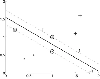
By considering a set of linear separators with the same orientation (parallel to one an-other), the distance between the separators that are further apart will constitute a margin. In this regard, among all possible separating lines with various orientations, one will have a maximum margin. The data points that define the boundaries of the lines composing the maximum separators are called support vectors. The concept is shown in figure2.2.
Figure 2.2: For a two class problem, the thick line defines the boundary and the dotted lines the limit of the margin on both sides. The dot and plus signs represent the classes, the ones encircled are the support vectors [Alp10].
C H A P T E R 2 . S TAT E O F T H E A R T
The main idea behind the SVM algorithm is therefore to identify the g(x) = 0 linear separator with the maximum margin of separation.
The logic behind this is that the maximum margin separator is the optimal separator, as classifiers with lower margins have demonstrated a higher associated risk of misclassi-fication.
When a set of data points cannot be linearly separated, a strategy called kernelling can be employed, where the number of dimensions is increased to try and find a linear separation in a higher dimensional space. Since the number of features determines the dimension of the input space (the data points), in order to obtain a higher dimension a new feature is computed based on the already existent features through a kernel function. Consequently, if a linear separation is attained at a higher dimensional space of n + 1 dimensions, the resulting separator in our n dimensional input space will be an hyper-plane. However, it may happen that no amount of higher dimensions will be capable of separating the data points, in which case an hyperplane that minimizes the error has to be selected [Bur08].
Due to the general use of more than three features, it is not possible to visualize or understand the resulting vector data, as it resides in a Euclidean space of high dimension. Although SVMs were initially considered, such techniques do not scale well with a large amount of samples. After encoding protein data into samples, a total of 3.282.479 sam-ples were obtained. This number would result in very slow training times, especially considering the large number ofhyperparametersto optimize.
2.4.3 Neural Networks
Neural networks are inspired by the brain. Since brains are able to learn, then, under-standing them and copying their learning mechanisms should be of use to the machine learning field.
The brain is very complex, but its building blocks, the neurons, may be described in a simplistic way that approximates their behavior. Basically, the neuron is an electri-cally excitable nervous cell that transmits information through electrical impulses. An impulse is fired when the electric potential within the neuron rises above a certain thresh-old. Neurons can connect to each other through synapses and are typically connected to thousands of other neurons on two different ends, a receiving end, where impulses are collected from the connected neurons through branches called dendrites, and a giving end (axon), where its own impulse is sent to the other connected neurons. Together, they form a neural network.
Each neuron can be visualized as a separate processor that performs the simple com-putation of deciding whether or not to fire [Mar09], allowing it to be simulated on a computer. By interconnecting the artificial neurons together we obtain the neural net-works machine learning technique.
2 . 4 . M AC H I N E L E A R N I N G
In order to simulate the neuron, although simplistically, a mathematical model was intro-duced in 1943 to describe the bare essentials of its operation. A neuron is thus modeled as:
1. A set of weighted inputs wi, meant to model the synapses (different synapses
con-tribute differently)
2. An adder that sums the input signals (simulates the collection of electrical charge in the cell)
3. An activation function responsible for deciding whether or not a neuron fires (thresh-old)
A set of input nodes {x1, ..., xm}are fed into the neuron. They represent impulses coming from the synapses of the connected neurons. Each x takes a value, 1 means that the input neuron fired and 0 that it did not. They can also take up values like 0.5, despite not having a biological meaning. Synapses coming into the neuron have different strengths associated with them, represented by the weights. Hence, the strength gathered from input signals is calculated by
h =
m
X
i=1
wixi, (2.6)
If a weight wi is 0, the corresponding input signal xi is irrelevant for our neuron. If it
is positive, it contributes towards firing by increasing the strength within the neuron, otherwise, if it is negative, it has an inhibitory effect. The altering of the weights allows the neuron to learn. Lastly, the neuron has to decide if it is going to fire, and that is if the collected strength surpasses a given threshold θ. If θ = 0, the neuron fires whenever
h > 0. Therefore, this simple activation function translates to g(h) = 1, if h > θ. 0, if h ≤ θ. (2.7)
In the neural network, these neurons are typically arranged in layers. The input layer directly collects the inputs from the system, while the output layer provides the final results of the computation. Hidden layers exist between the former and the latter, collect-ing inputs from the previous layer and providcollect-ing output to the next layer [Mar09].
Neural Networks can work really well, but they are time consuming to set up due the vast amount ofhyperparametersand the very long time required to train. This does not make a good candidate for validating against different homolog settings.
2.4.4 Logistic Regression
Despite having regression in its name, Logistic Regression is a classification model. Likely due to the fact that it uses the output of a logistic function, commonly known as sigmoid function, to decide whether a given sample belongs to a class.
C H A P T E R 2 . S TAT E O F T H E A R T
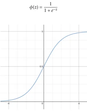
The sigmoid function has a characteristic S-shape2.3, as it is defined by the formula
2.8.
φ(z) = 1
1 + e−z (2.8)
Figure 2.3: Sigmoid activation function.
This function converts any real number into the [0,1] range. Thus, when z is the the linear combination of the m features and their affected weights, z = wTx = w
0x0+ w1x1+ . . . + wmxm, the output can be interpreted as a probability of sample x belonging to the positive class [RM17].
The classifier is simple in itself, but it is one of the most widely used algorithms in the industry and it generally provides good results.
Its simplicity is a strong point, as it requires little configuration and is fast to train. It is therefore very suitable to use for the particular problem in this thesis where models have to be optimized and trained from the beginning with each different data configuration. 2.4.5 Naïve Bayes Classifier (NBC)
Naive Bayes models have been particular successful at the problem of information re-trieval [Lew98; MN98], which makes it an interesting choice due to its similarity with contact prediction, where the disproportion of contacts in relation to non contacts re-semble that of the disparity of relevant documents against non relevant documents when making a query on a search engine.
Unlike the previous classifiers, NBC follows a generative model and assumes that all features are independent of each other given the context of the class, i.e. conditionally independent. Probabilities are associated to each feature given the class, carrying out the
![Figure 1.1: Anatomy of an amino acid [Bur08].](https://thumb-eu.123doks.com/thumbv2/123dok_br/15485794.1039692/29.892.272.618.637.817/figure-anatomy-of-an-amino-acid-bur.webp)
![Figure 1.2: The four levels of protein structure [Bra+99].](https://thumb-eu.123doks.com/thumbv2/123dok_br/15485794.1039692/31.892.231.664.704.859/figure-levels-protein-structure-bra.webp)