DOCUMENTOS DE TRABALHO
WORKING PAPERS
GESTÃO
MANAGEMENT
Nº 02/2009
THE USE OF THE R
2AS A MEASURE OF FIRM-SPECIFIC
INFORMATION: A CROSS-COUNTRY CRITIQUE
Paulo Alves
Universidade Católica Portuguesa (Porto) and Lancaster University
Ken Peasnell
Lancaster University
Paul Taylor
The use of the R
2as a measure of firm-specific
information: A cross-country critique
Paulo Alves1 Ken Peasnell2 Paul Taylor2 23 December 2008
Abstract
Recent research uses the degree of stock returns co-movement as a measure of the quality of a country’s information environment. It has been argued that stronger property rights, better corporate governance regimes and more efficient enforcement mechanisms lead to prices incorporating more firm-specific information and, therefore, co-moving less with the market. In this paper, we use a much more comprehensive international data set than in prior research, encompassing forty countries over twenty years, to evaluate the reliability of this approach in a cross-country setting and to analyse the behaviour of the measure used. Our results demonstrate severe limitations in the use of co-movement as measure of information quality. We highlight the instability of the measure and show that it can produce results that are often difficult to reconcile with such an informational explanation.
Keywords: Information; R²; firm-specific information; market-wide information;
volatility; disclosures; co-movement; cross-country information environment.
1
Portuguese Catholic University and International Centre for Research in Accounting (Lancaster University Management School): p.alves@porto.ucp.pt
Financial support was provided by Fundação para a Ciência e Tecnologia – Portugal (ref. SFRH/BD/9147/2002).
2
Lancaster University, Management School
Address for correspondence: Paulo Alves, Lancaster University Management School, Lancaster LA1 4YX, United Kingdom. Comments and suggestions from seminar participants at the 30th European Accounting Association (Lisbon), Lancaster University (UK), London School of Economics (UK), Portuguese Catholic University (Portugal) and Warwick University (UK) are gratefully acknowledged. We are particularly indebted to David Ashton and Martien Lubberink for their valuable comments and suggestions. Finally, we are grateful to the Institutional Brokers Estimate System (I/B/E/S), service of Thomson Financial, for providing us with the data as part of a broad academic program to encourage earnings expectations research.
1. Introduction
Morck et al. (2000, 215) claim that “stock prices move together more in poor economies than in rich economies”. Rich economies tend to have stronger property rights, better corporate governance regimes and more efficient enforcement mechanisms, all of which promote arbitrage trading based on information about a firms‟ fundamentals. In the presence of such an information environment, they argue, prices will incorporate more firm-specific information and, therefore, co-move less with the market.
The study of the quality of information environments at the cross-country level is of major relevance to both the investing community and regulators. Barriers to international trade are vanishing and at the same time capital mobility has been increasing and, therefore, investors need more country-specific information and a better understanding of international stock markets. At the same time, regulators are endeavouring to make strong efforts to harmonise both capital market regulations and financial reporting rules. The study of these matters helps us to understand the information dynamics, both within a country and at the cross-country level, and therefore hopefully will facilitate the formulation of more informed regulation.
Morck et al.‟s (2000) approach uses the average R² for a country of a regression of a company‟s stock returns on overall stock market returns as a proxy for the quality of a country‟s information environment. The appeal of this approach is that it seems to provide a simple measure to evaluate the complex concept of information quality. The R² methodology has an intuitive logic behind it. In the extreme case where firm-level information is so poor that investors cannot distinguish between companies, they will be forced to treat them as essentially the same. Market-wide
information will then be the major factor driving price changes, with consequently high R²s being observed.1 High R2s might also be observed in a market where firms are generally large and well-diversified. On the other hand, if firms are generally focused in particular lines of business or where good sources of reliable firm-specific information are available then firms will not be viewed as substitutes by investors and R2s should be small. This intuition underpins the use of R² as a metric for ranking countries according to the quality of their information environments.
Most subsequent research in this area takes for granted the reliability of R2 as a measure of information. This paper critically analyses such use of R² at the cross-country level. We show that such an informational interpretation of R² has to be treated with great care. We apply the R² methodology in a cross-country setting using a very comprehensive data set we have collected based on forty countries over the twenty-year period 1985-2004. Our results demonstrate clearly the inadequacy of the R² as a measure of the quality of the information environment. When attempting to measure the quality of firm-specific information at the country-level, there are many confounding factors to be accounted for, 2 raising severe doubts as to whether it is possible to encapsulate such a multiplicity of factors in a single measure.
Our approach can be summarized as follows. First, we rank countries according to their average R² for the whole period. We then consider whether the resulting ranking can be reconciled with what is generally known about the financial
1
In the limit, a pooling equilibrium would prevail, with attendant risks of a “market for lemons” that might cause a breakdown in the market (Akerlof 1970). Very poor information environments are thus likely to limit the growth of stock markets. In keeping with prior research in this area, we do not consider such endogeneity issues any further in the present study.
2
For instance: size of the country, size of capital markets, type of economy, investor property rights, corruption levels and the role of government in the economy.
environments of the countries involved. Whilst the ranking presented by Morck et al. (2000) for the single year of 1995 is certainly plausible in terms of its association with certain country economic and legal variables, our ranking based on the average for the whole 20 years is very different and presents a puzzling picture. Furthermore, the annual R² for a single country changes considerably from year to year, a fact which is hard to reconcile with the argument that corporate governance and investors‟ protection regimes are driving its behaviour. Such a relationship would only be possible if these factors change with rapidity and frequency, improving one year and falling back again in the next, circumstances which are highly unlikely.
To explore this further, we examine the spurious effects of aggregation and decomposition on the R² measure. We do this by artificially aggregating and decomposing real countries to create pseudo-countries and analyse their impact on the R² measure. When we create a bigger „country‟ by „merging‟ two smaller ones, we find that the resultant R² falls dramatically. We also explore the converse, by breaking a single country, the USA, into smaller pseudo-countries defined by the particular US stock market in which a firm is listed. We find that the R² of each pseudo-country is larger than that for the USA as a whole. By construction, these effects cannot be explained in terms of changes in the quality of the information environment or in the factors that Morck et al. (2000) claim to be driving R², i.e. corporate governance and investors‟ protection regimes.
The remainder of the paper is organised as follows: The next section reviews the literature and section 3 discusses our sample and the metrics used in the chapter. Section 4 empirically explores the cross-country setting by analysing in the different ways described above anomalies in the R² as a measure of information environment
quality. Finally, section 5 draws conclusions and establishes the path for future research.
2. Prior research
In this section, we outline the rationale underlying the R² methodology as a measure of information quality and explain how it has been used in empirical research. We then establish a context for the present study by summarising the growing body of work criticising the R² methodology.
Morck et al. (2000) argue that strong property regimes provide the economic conditions conducive to information-driven arbitrage trading based on firms‟ fundamentals. As these conditions are generally found in developed countries and less so in developing ones, the stock prices of the former are more likely to incorporate more firm-specific information. Their study uses a methodology first introduced by Roll (1988) to test the ability of asset pricing theory to explain ex-post stock returns based on pervasive factors, industry influences and events unique to the firm.
Roll (1988) uses a regression of company returns on market and industry returns3 and interprets the coefficient of determination (R²) of this regression as an inverse proxy for firm-specific information. High (low) R²s indicate that company returns are being explained more (less) by pervasive factors compared to firm-specific factors. To test if the unexplained component was the result of firm-specific information, Roll ran the regression again excluding observations on the dates on
3 Roll‟s (1988) initial model has only market returns as an explanatory variable. The industry factor is
added to improve the model‟s coefficient of determination and, therefore, results in a more refined measure of firm-specific information. Roll (1988) uses the one factor CAPM and the multi-factor APT model; both models produce similar results.
which information about the firm or its industry appeared in the public domain. If the residuals were capturing firm-specific information, the R² of the second regression should be considerably higher. However, he found that deleting those dates did not increase R² significantly. Roll (1988, 566) concludes that an “occasional frenzy unrelated to concrete information” was driving the results. Despite subsequent attempts to improve the methodology (Brown 1999; Cornell 1990; Robin 1993), his conclusion remains uncontested.
A new stream of research uses such R² methodology. Morck et al. (2000, 216, emphasis added) state that “[a]s Roll (1988) makes clear, the extent to which stocks move together depends on the relative amounts of firm-level and market-level information capitalized into stock prices”. A close reading of Roll‟s paper suggests that this is a questionable interpretation of his findings. Nevertheless, Morck et al. (2000) show that R²s are higher in countries with poorer economies that are often characterised by weaker corporate governance and investors‟ protection mechanisms, as measured by a “good government index” based on La Porta et al. (1998).4
In the presence of weak property rights, information-based trading becomes less attractive, less firm-specific information is capitalised and, therefore, more stock price synchronicity is observed.
Subsequent cross-country and firm-level research appears to corroborate these results. Jin and Myers (2004) find that countries where firms tend to be more
4 Morck et al.‟s (2000) research finds a significant and negative association between R² and countries‟
GDP. They hypothesise that GDP might be proxying for specific economic characteristics affecting stock price synchronicity. To test this hypothesis, the R2 stock price synchronicity measure is regressed on the natural log of the number of shares in the market, the country‟s GDP and a vector of structural economic characteristic (macroeconomic volatility, country size, economy diversification and earnings co-movement). All structural variables fail to mitigate the statistical significance of GDP. In contrast, the inclusion of the “good government index” makes the GDP coefficient statistically insignificant.
opaque5 have higher R² and higher frequencies of crashes. Control rights and the opaqueness of information affect managerial behaviour and, therefore, higher R²s are associated with countries having less developed capital markets and weaker corporate governance regimes.
Li et al. (2003) find that R² is negatively associated with the degree of openness6 of capital markets. They also find that the negative relationship only holds when the countries have strong corporate governance regimes; otherwise, the relationship is positive. They do not put forward a well-developed explanation for this contradictory result.
There is also a growing body of literature using the R² measure at the firm-level (e.g. Durnev et al. 2001; Durnev et al. 2003; Fox et al. 2003; Piotroski and Roulstone 2004). Most of this literature uses the R²-methodology as proposed by Morck et al. (2000) without questioning its reliability. More recently, the informational interpretation of R² has been subjected to detailed scrutiny, particularly at the firm-level. Ashbaugh-Skaife et al. (2005) confirm Morck et al.‟s (2000) findings for a smaller set of countries but strongly disagree with their interpretation of the results. Ashbaugh-Skaife et al. (2005) document the non-existence of a relationship between R² and a set of variables capturing some of the firm‟s characteristics, which might be expected to capture aspects of the quality of its information environment, such as analyst forecast errors, firm size and stock turnover. Their results lead them to conclude that R² is not associated with firm-specific information and, therefore,
5 In their model, opaqueness refers to the lack of transparency between managers and investors. 6
Openness is defined as the value of stocks that can be purchased by foreign investors as a percentage of total domestic market capitalization.
cannot be used to compare countries based on an informational explanation. These results are reinforced by Kelly (2005), who arrives at similar conclusions, showing that the R² is not related to firm-level fundamentals that theory and evidence suggest are predictive of the quality of a firm‟s information environment (e.g. firm size, age, institutional ownership, analyst coverage and liquidity).
While most of the criticism has focused on the use of R² at the firm level, the results at the cross-country level have received less attention. Our study focuses specifically addresses the reliability of the measure at the country level.
3. Metrics and sample construction
In order to assess the validity of R² as a measure of firm-specific information, we use regression to capture the level of stock returns explained by the market. We adopt the usual practice in cross-country studies using the R² methodology of not including an industry variable in the model because of the attendant difficulties in defining industries in countries with small capital markets (the majority of the sample). Unlike Morck et al. (2000), we do not include US stock market returns as a variable because exposure to the US market is better viewed as having two components, one being firm specific and the other as market-wide, the latter being captured by the market variable and the former by the residuals.
Our model, expressed in Equation (1), regresses company j’s returns (RCjwt) on market‟s returns (RMjwt) and yields a R2 value per company-year.
jwt jwt jt jt jwt RM RC (1)
To mitigate thin trading problems, all returns are measured on a weekly basis (w) for each year (t). To prevent spurious correlations – more severe in countries with
few companies – market returns are value-weighted averages excluding company j, as follows:
n j i i iwt n j i i iwt iwt jwt RC MV MV RM 1 1 (2)where RMjwt is the market return in week w of year t, excluding firm j, MViwt is company i’s market value for the same period and n is the number of companies in the market. RCiwt is company i‟s returns in week w of year t.
R2 is the proportion of the regression sum of squares (SSR) to the total sum of
squares (SST), which is in turn the sum of SSR and the sum of squared errors (SSE).
jt jt jt jt jt jt SSE SSR SSR SST SSR R 2 (3)
An annual R² value for the entire sample is then computed by weighting individual R2s within country c by SST, as in Equation (4) below. We adopt this approach for purposes of comparison with prior work and because it allows us to apply the same rationales as in Equation (3) to the country level and to facilitate the decomposition of the aggregate R² into its components:
c j jt c j jt jt ct SST SST R R 2 2 (4)Large R2s indicate that the market explains a substantial proportion of the company‟s returns. Under the informational interpretation used by Morck et al. (2000) and Durnev et al. (2001), a small R2 means that such pervasive factors poorly explain the company‟s returns and, therefore, firm-specific information is driving the measure. These rationales when applied at the country-level suggest that in countries with high
(low) R²s market-wide factors are more (less) relevant in explaining stock returns relative to firm-specific information.
Our sample comprises data for the same forty countries used in Morck et al. (2000), for comparability, but covering a much longer period, 1985-2004. These countries form a comprehensive set of active capital markets that are representative of capital markets worldwide.
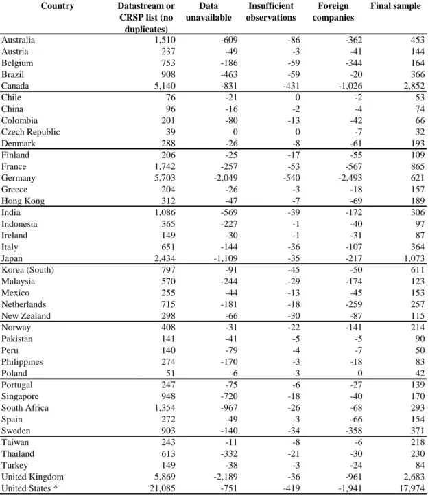
For each country, we select the most comprehensive list of companies available in the database. We eliminate all duplicate records, both within and across countries (cross-listed companies). When deleting cross-country duplicates, we retain the observation from the country of origin. We exclude secondary issues of shares, companies without information available, and companies that for a particular year have less than 26 weekly observations for returns. Finally, to mitigate the influence of extraneous environmental and governance factors, we exclude companies classified as foreign for a particular market. Table 1 presents details of the composition of the final sample.
Table 2 shows the number of companies per year in each country. The number of firms varies significantly across countries. Poland has the least firms, with an average of only 27 companies, and the USA has the most, with an average of 6,624 companies. The overall average per country is 342 companies (181 if we exclude the USA) and the median is 96 companies. There are missing data for earlier years for some countries. We deal with this missing-data problem by running our tests both for the whole period and for the period for which common data are available for all countries (1997-2004). We delete years when the number of firms in a country is
below 20% of its average for the whole period.7 All information was retrieved directly from CRSP (USA) and Datastream (all other countries) and it includes dead and financial companies.
A final difference between our sample and Morck et al.‟s (2000) is that we do not exclude extreme returns. In their study, all bi-weekly stock returns higher than 25% in absolute value are excluded as data errors. Untabulated detailed investigations in the UK suggest that these are more likely to reflect important new information and as such are not simply due to measurement error.8 Our reason for not excluding such outlying observations is to ensure all information effects are properly captured.
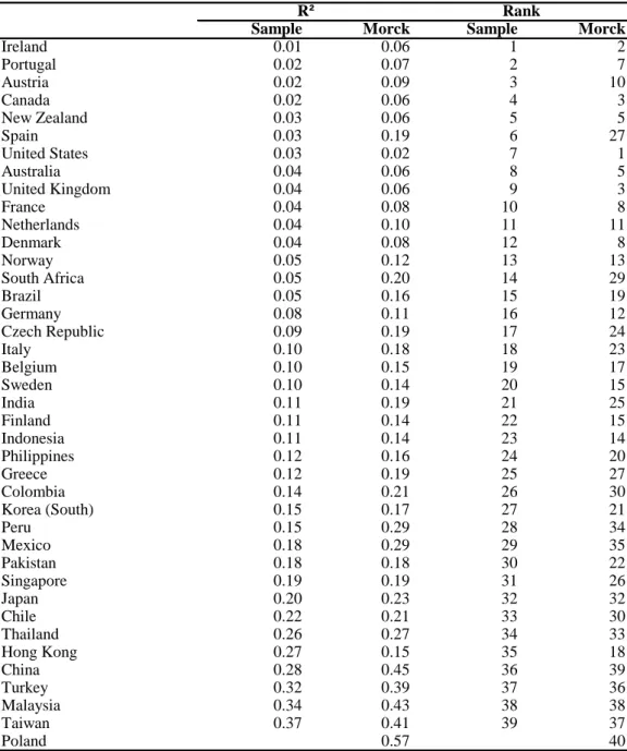
Table 3 compares results for the year of 1995 used in Morck et al.‟s study to check consistency between our results and their‟s. It shows, as expected, R²s in our sample are considerably lower than Morck et al.‟s. We rank the two sets of results and run two nonparametric measures of association (Sheskin 2004). Both Kendall‟s tau and Spearman‟s rho show a large degree of concordance, 0.75 and 0.83, respectively, both significant at the 0.01 level, allowing us to conclude that there is a monotonic positive relation between the ranks in our study and that of Morck et al.‟s (2000). As a further sensitivity check, we also re-ran the analyses reported below, using a model identical to Morck et al.‟s that included US returns with exactly the same trimming of extreme returns at 25%. Untabulated results indicate that our overall results reported below remain substantially unaffected.
7
As a robustness check, we also replicate this sample selection criterion at 10% and 25%. Our results are not statistically sensitive to the choice of cutoff point.
8 In particular, we examined actual information releases for our complete sample of UK companies
during the week in which the extreme returns were observed. We used the Perfect Information database and selected all returns above 200%. In 87% of the cases there was an information release about the company.
4.Results
4.1. Ranking countries
We rank countries by their mean R² over the sample period to see if such rankings accord with commonly-held preconceptions of the quality of countries‟ information environments. In Table 4 – Panel A, we can immediately determine that the rank produced based on the mean (last column) is inconsistent with an informational explanation. The Czech Republic and Portugal are in the top five and as such almost as good as the USA. Peru would be interpreted as having better corporate governance and investors‟ protection regimes than the UK, with Pakistan as being near equal to Japan, and both far better than Hong Kong. Table 4 – Panel B ranks countries by individual year. The rankings exhibit considerable variability across time.
As a robustness test, Table 4 ranks the countries according to the R² average for the common data period (1997-2004) rather than the whole period. Conclusions are even more puzzling for this sub-sample. Now the USA, generally acclaimed as the strongest capital market in the world, is only in eleventh place, behind countries like Austria, Belgium, Czech Republic, Ireland, Peru and Portugal.
Clearly, whichever data set is used, the cross-country ranking of R2 is extremely sensitive to the choice of year. Furthermore, one can observe from Table 4 – Panel B that for some countries R² is erratic over time. If corporate governance and other macro-economic factors are deemed mainly to explain the behaviour of the R² measure, then we would not expect to observe such extreme fluctuations as the ones shown. There are 696 adjacent-years-country possible paired combinations. In 171 pairings we observe an increase of at least 100% or decreases of more than 50% in
annual R². The number goes up to 324 pairings if we consider increases of at least 50% and decreases of 33% or more in R².
To test if the overall differences in R² from year to year are statistically significant, we apply a Single-Factor Within-Subjects Analysis of Variance based on the null hypothesis that the mean R² between years in the sample is constant.9 Untabulated results show that, after removing the country effect, the null hypothesis is rejected at both the 0.05 and 0.01 levels, confirming that that there is a significant difference between the mean R² for at least two of the years. These results hold both for the whole sample and for the common sample. 10
We also examine whether there are significant changes between overall average R² for adjacent years. Untabulated results reveal that for 14 (10) out of the 19 year pairs the null hypothesis that overall average R²s remain stable is rejected at the 0.05 (0.01) level. Again, applying the same test to the common data years results in the rejection of the null hypothesis for 5 (4) out of the 7 year pairs at the 0.05 (0.01) level, respectively.
4.2. Effects of aggregation and decomposition
If R² is to serve as a reliable measure of the information environment it should not be affected unduly by the arbitrary aggregation of or subdivision of countries when selecting a measure of market returns. We address this issue by
9
This test is a multivariate analogue of the paired sample t test for means and it increases the power of the test by examining the extent of the differences in mean annual R² for years (between „conditions‟) after removing the effect of the countries (between „subjects‟).
10 We also apply the non-parametric Friedman Two-Way Analysis of Variance by Ranks test (Sheskin
2004) to the country ranks shown in Table 4 – Panel B in order to test if at least two medians are different, with essentially the same results.
presenting the results of creating R2 for „pseudo-countries‟ obtained by aggregating real countries based on different criteria described below and comparing it with the average of the R2 for the original non-aggregated countries. We then explore the inverse approach by decomposing the American market into its three main stock exchanges.
Equation (5) represents the baseline we use to compute the R² for a single country. In this equation, the returns of firm i in country j (Rij) are regressed on the market returns of country j, and then weighted by SST for the combined countries together to get the R2 for the whole pseudo-country:
ij j j j ij RM R . (5)
The same equation is used to compute the R² for a given Pseudo-Country. In this case, the pseudo-market return, RM, is generated using all companies in the n original country markets included in the Pseudo-Country. Fitting one model for n combined countries would result in a single composite index analogous to a value-weighted average of the individual countries, as shown in Equation (6):
n n n n
ii wRM w RM w w RM
R 1 1... 1 1 1 1... 1 . (6)
In concept, fitting separate models for each country could be viewed as analogous to (but not quite the same as) fitting a single regression model with dummy intercepts and slopes for each country, as in Equation (7):
i n n n n n i D D RM RM D RM D R 12 1... 11 12 2 1... 1 . (7)
To the extent that the dummy variables are significant, and the explanatory power of the markets is differentiated, this model would result in a better fit. On the other hand, only if all the dummy variables were insignificant and the different
markets had no differential explanatory power, would the resulting R² be similar to the one yielded by Equations (5) and (6).11
4.2.1. Examples of the effects of aggregation
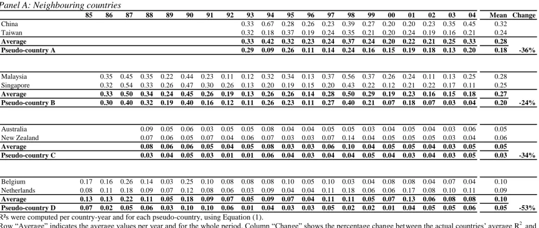
Based on our data set, we provide some numerical examples to illustrate the effects of aggregation of countries on R2 discussed above. First, Table 5 - Panel A illustrates the effects of combining two neighbouring countries to form a larger pseudo-country. Morck et al.‟s analysis would not lead us to expect a significant change in R2 as a result of this merger because the information environment has not changed. Therefore, if R² is a good measure of such a quality, we would expect R²s pre- and post-merging to be an average of the two. However, when we perform such a procedure based on our data, we consistently observe a drop in R². Consider for instance Belgium and Netherlands with R²s of 10% and 9%, respectively. The merging of these two capital markets decreases R² by 53% to 5%. If we follow Morck et al.‟s (2000) interpretation, the merging of the two countries would be interpreted as a significant increase in the strength of corporate governance and investor protection regimes and, therefore, in the overall quality of the information environment. For illustrative purposes, we applied the same procedure to other geographically neighbouring countries with similar results: China and Taiwan would „increase‟ the quality of their information environment by 36%, Malaysia and Singapore would observe an „improvement‟ of 24% and, finally, Australia and New Zealand of 34% .
11
Fitting a separate model for each country assumes country effects are independent of each other. It could be the case, for example, that returns in one country may be affected by the index in another, resulting in the following equation.
i n n n n i D D RM RM R 12 1... 11 1... . This aspect is not considered in this paper.
Second, the same effect is observed if we combine any countries with very similar R2, details of which are given in Table 5 – Panel B. Pseudo-country E, for example, includes six countries (Ireland, New Zealand, Peru, United Kingdom, Brazil, and Australia), all with an R²s between 0.06 and 0.07; by merging them we observe a 40% reduction in R². Other similar combinations show even larger reductions in R2. Pseudo-country F (Germany, India, South Africa, Finland, Indonesia and Sweden), for example, which also has a variation in R2 between the original constituent countries of only 0.01, has a 74% reduction in R².
Finally, we also examine the behaviour of R2 where pseudo-countries are created by merging actual countries based on a non-R2-based selection criterion. In particular we use similarity of scores in the S&P transparency and disclosure ratings (Doidge et al. 2004). The results, reported in Table 5 – Panel C, are similarly inconsistent. This final ranking could be regarded as particularly compelling, given that the basis of combination provides us with an externally determined measure of some common dimensions of a each country‟s corporate governance quality. Again, the aggregation of these information-environmentally similar countries has resulted in approximately a 50% reduction in R².
The above examples demonstrate that aggregation reduces R². The reason is that instead of fitting n models, one per country, to determine R² we are now fitting only one model to n countries. We are effectively forcing the parameters to be the same across the n populations, as demonstrated analytically in the previous section. If the parameters in the separate models are significantly different, the aggregated model
loses part of its ability to fit the data and a lower R² results. In all the above examples, untabulated Wald tests reveal that these parameter restrictions are highly significant.12
4.2.2. An example of the effects of disaggregation
We now adopt the opposite procedure by disaggregating one country, the USA, into three pseudo-countries, each corresponding to the three major stock exchanges (AMEX, NASDAQ and NYSE). We know, of course, that each pseudo-(subdivided) country has almost the same institutional framework. Needless to say, there are some differences. A large portion of the companies listed in the AMEX are smaller than those in the other two stock exchanges. The NASDAQ is the largest stock exchange in terms of number of companies listed and number of shares traded per day. It has a strong focus on new technology and R&D intensive firms. The NYSE is by far the largest in dollar traded volume and second largest by number of companies listed. The NYSE is often referred as representing the Old Economy and the NASDAQ as representing the New Economy. Table 6 – Panel A presents the number of companies per year and per stock exchange.13
In spite of these differences, all are under the regulatory umbrella of the SEC, and apply the same accounting GAAP. All have a similar analyst environment and corporate governance and investors‟ protection regimes. However, if we look at Table 6 – Panel B without knowledge of the name of the particular stock exchange (as if the R²s were from different countries), we would conclude that the country called NYSE has the worst information environment of the three because it has the highest R2. The
12 Significance levels are high. 70% are significant at the 1% level.
13 Bennett and Sias (2004) attribute the increase in firm-specific risk over the last three decades to the
growth of riskier industries, the increase of small stocks in the market and a decline in industry concentration. These types of companies are much more frequently found in AMEX or NASDAQ.
other two „countries‟ have somewhat similar R2
s. It could be argued that we ought to observe the opposite ranking: the NASDAQ and AMEX comprise smaller and more technology-intensive companies. Smaller companies will be less closely followed by analysts and might have less sophisticated governance regimes. The value of technology-intensive companies will be subject to greater uncertainty because they are more dependent on growth options. For both types of company, these factors might lead one to conclude that they have worse information environments and, as such, ought to have higher R2s. In passing, one might also note the similarity in R2 of the NYSE with the South American country, Colombia (see Table 3 – Panel A). It is difficult to believe that the information environments of the NYSE and the Bogota Stock Exchange are of similar quality.
5. Conclusions
The paper presents a cross-country analysis of the use of R² as a measure of information. Our results lead us to conclude that R2 is inadequate as a measure of the quality of the information environment at a country level. The rationales advanced in the literature for the use of R² as a measure of information have been based on the implicit assumption of stability of country corporate governance and investor protection regimes. It is inconceivable that such factors could change as rapidly and unpredictably as do the changes in R2. Our study also reveals substantial aggregation and disaggregation problems with R2 as a measure of the quality of the information environment at a country level.
The usefulness of a single indicator of the quality of a firm‟s information environment is beyond question. However, our research indicates that R2 is an unreliable metric for this purpose.
Table 1 –Number of companies per country (1985-2004)
* For the US, secondary issues of shares were, for presentation reasons, classified as “data unavailable”. Country Datastream or CRSP list (no duplicates) Data unavailable Insufficient observations Foreign companies Final sample Australia 1,510 -609 -86 -362 453 Austria 237 -49 -3 -41 144 Belgium 753 -186 -59 -344 164 Brazil 908 -463 -59 -20 366 Canada 5,140 -831 -431 -1,026 2,852 Chile 76 -21 0 -2 53 China 96 -16 -2 -4 74 Colombia 201 -80 -13 -42 66 Czech Republic 39 0 0 -7 32 Denmark 288 -26 -8 -61 193 Finland 206 -25 -17 -55 109 France 1,742 -257 -53 -567 865 Germany 5,703 -2,049 -540 -2,493 621 Greece 204 -26 -3 -18 157 Hong Kong 312 -47 -7 -69 189 India 1,086 -569 -39 -172 306 Indonesia 365 -227 -1 -40 97 Ireland 149 -30 -1 -31 87 Italy 651 -144 -36 -107 364 Japan 2,434 -1,109 -35 -217 1,073 Korea (South) 797 -91 -45 -50 611 Malaysia 570 -244 -29 -174 123 Mexico 255 -44 -13 -45 153 Netherlands 715 -181 -18 -259 257 New Zealand 298 -66 -30 -87 115 Norway 408 -31 -22 -141 214 Pakistan 141 -41 -5 -5 90 Peru 140 -79 -4 -7 50 Philippines 274 -170 -3 -18 83 Poland 51 -6 -3 0 42 Portugal 247 -75 -6 -27 139 Singapore 948 -720 -18 -40 170 South Africa 1,354 -967 -26 -68 293 Spain 272 -49 -3 -66 154 Sweden 903 -140 -34 -358 371 Taiwan 243 -11 -8 -6 218 Thailand 613 -332 -21 -30 230 Turkey 149 -38 -3 -24 84 United Kingdom 5,869 -2,189 -36 -961 2,683 United States * 21,085 -751 -419 -1,941 17,974
20
Table 2 –Number of companies per year (1985-2004)
Nr Country 84 85 86 87 88 89 90 91 92 93 94 95 96 97 98 99 00 01 02 03 04 Mean 1 Australia 75 75 78 81 114 135 148 157 181 199 236 255 292 300 292 279 277 270 243 244 217 204 2 Austria 24 24 26 34 39 43 48 61 73 86 94 101 100 100 103 94 90 90 80 73 59 71 3 Belgium 46 48 71 76 79 81 84 90 91 92 97 98 104 111 118 121 126 123 117 109 99 97 4 Brazil 17 35 45 50 64 196 189 245 241 242 234 202 171 142 112 146 5 Canada 284 322 366 433 475 975 1,285 1,284 1,155 1,136 1,231 1,235 1,223 1,262 1,345 1,296 1,261 1,131 847 612 419 965 6 Chile 30 31 34 38 39 40 40 44 46 45 45 45 46 47 47 41 7 China 5 11 21 26 31 49 56 57 59 57 49 50 47 40 8 Colombia 25 33 34 43 47 49 48 44 48 44 44 44 42 42 9 Czech Republic 7 30 31 31 32 32 32 32 32 32 30 29 10 Denmark 40 41 44 44 105 118 121 125 149 153 155 161 170 161 160 143 129 108 85 73 62 115 11 Finland 3 29 34 39 49 49 53 60 73 77 84 89 92 82 74 67 59 51 59 12 France 99 103 107 113 153 353 374 427 439 450 495 530 559 655 628 501 476 456 408 337 269 392 13 Germany 130 133 142 150 157 285 323 349 373 386 396 411 448 434 438 449 472 454 431 367 294 345 14 Greece 55 59 69 85 88 88 101 112 114 116 114 101 99 96 80 69 59 89 15 Hong Kong 46 49 51 57 80 84 85 87 98 114 122 126 132 138 139 137 139 137 135 126 128 108 16 India 128 143 153 186 229 237 253 246 227 194 141 129 126 118 109 175 17 Indonesia 29 38 43 46 51 61 67 75 78 73 68 65 62 57 56 58 18 Ireland 32 34 36 41 51 58 60 62 63 62 63 62 63 65 68 70 70 66 60 54 53 58 19 Italy 53 54 139 187 199 214 224 231 241 242 248 249 254 245 230 231 230 216 207 181 159 209 20 Japan 356 356 357 359 528 581 703 746 767 778 807 844 872 883 885 874 830 791 734 654 581 697 21 Korea (South) 2 119 123 133 160 206 274 283 286 288 293 296 305 367 362 332 366 336 307 256 178 264 22 Malaysia 12 12 58 62 65 66 72 77 84 92 95 98 101 110 111 108 103 102 98 93 90 85 23 Mexico 31 37 47 53 79 88 102 102 99 84 83 73 76 80 84 85 88 76 24 Netherlands 104 112 119 133 140 146 154 159 164 167 172 176 185 196 214 220 207 179 163 148 138 165 25 New Zealand 5 6 36 36 38 38 45 53 66 72 71 65 69 69 68 74 67 61 58 52 26 Norway 31 37 41 44 43 47 65 68 70 76 92 104 119 132 146 132 114 99 90 60 50 81 27 Pakistan 3 4 56 60 67 71 71 81 80 77 74 65 61 49 59 28 Peru 2 12 18 21 30 35 36 38 38 42 47 46 42 42 32 29 Philippines 6 6 32 38 43 49 56 64 70 70 63 60 53 53 51 48 45 47 30 Poland 3 5 13 22 32 35 39 40 41 42 27 31 Portugal 46 57 70 76 82 91 96 103 105 103 111 101 90 72 62 56 51 81 32 Singapore 58 58 59 62 68 74 80 88 94 101 109 112 114 119 122 119 123 116 100 98 93 95 33 South Africa 33 33 34 40 41 45 161 177 187 195 200 208 228 228 215 163 122 92 81 78 71 130 34 Spain 5 43 46 71 82 87 90 97 98 100 101 106 119 130 134 140 135 127 121 96 35 Sweden 36 39 43 46 48 104 129 136 143 152 168 190 204 212 220 221 205 186 163 111 88 140 36 Taiwan 18 23 57 62 75 91 97 100 124 132 139 153 157 154 138 119 95 102 37 Thailand 30 45 70 93 107 130 148 168 189 199 188 140 110 82 74 67 60 57 109 38 Turkey 22 24 32 45 50 53 54 58 58 65 69 68 74 73 71 51 49 54 39 United Kingdom 786 839 903 990 1,097 1,171 1,225 1,252 1,276 1,333 1,464 1,556 1,705 1,818 1,819 1,682 1,657 1,688 1,689 1,580 1,512 1,413 40 United States 5,907 5,832 6,007 6,470 6,452 6,225 6,167 6,050 6,254 6,551 7,237 7,361 7,820 8,034 7,917 7,348 7,137 6,520 6,006 5,594 5,495 6,624
Table 3 – Comparing R² as per Morck et al.’s (2000) study with those of the current study based on the only year used by that study of 1995
For the year 1995, Poland has less than 20% of the average number of companies for the whole period and, therefore, it was excluded from our analysis.
R² for our sample was computed using Equation (1) that differs from Morck et al.‟s (2000) model in that it does not include US market returns.
Sample Morck Sample Morck
Ireland 0.01 0.06 1 2 Portugal 0.02 0.07 2 7 Austria 0.02 0.09 3 10 Canada 0.02 0.06 4 3 New Zealand 0.03 0.06 5 5 Spain 0.03 0.19 6 27 United States 0.03 0.02 7 1 Australia 0.04 0.06 8 5 United Kingdom 0.04 0.06 9 3 France 0.04 0.08 10 8 Netherlands 0.04 0.10 11 11 Denmark 0.04 0.08 12 8 Norway 0.05 0.12 13 13 South Africa 0.05 0.20 14 29 Brazil 0.05 0.16 15 19 Germany 0.08 0.11 16 12 Czech Republic 0.09 0.19 17 24 Italy 0.10 0.18 18 23 Belgium 0.10 0.15 19 17 Sweden 0.10 0.14 20 15 India 0.11 0.19 21 25 Finland 0.11 0.14 22 15 Indonesia 0.11 0.14 23 14 Philippines 0.12 0.16 24 20 Greece 0.12 0.19 25 27 Colombia 0.14 0.21 26 30 Korea (South) 0.15 0.17 27 21 Peru 0.15 0.29 28 34 Mexico 0.18 0.29 29 35 Pakistan 0.18 0.18 30 22 Singapore 0.19 0.19 31 26 Japan 0.20 0.23 32 32 Chile 0.22 0.21 33 30 Thailand 0.26 0.27 34 33 Hong Kong 0.27 0.15 35 18 China 0.28 0.45 36 39 Turkey 0.32 0.39 37 36 Malaysia 0.34 0.43 38 38 Taiwan 0.37 0.41 39 37 Poland 0.57 40 R² Rank
22
Table 4 – R² by country-year
Panel A: Rank by average R² – Whole sample
R² is calculated per each country-year in the period 1985-2004 using Equation (1). Countries are then ranked by the average R² for the whole period available.
Rank Country 85 86 87 88 89 90 91 92 93 94 95 96 97 98 99 00 01 02 03 04 Median Mean
1 Canada 0.03 0.03 0.10 0.03 0.02 0.02 0.02 0.02 0.02 0.02 0.02 0.02 0.03 0.03 0.02 0.03 0.03 0.03 0.03 0.03 0.03 0.03 2 United States 0.03 0.04 0.09 0.03 0.03 0.04 0.04 0.03 0.02 0.04 0.03 0.03 0.03 0.06 0.03 0.11 0.08 0.06 0.05 0.08 0.04 0.05 3 Czech Republic 0.03 0.09 0.04 0.05 0.10 0.08 0.05 0.03 0.03 0.03 0.04 0.04 0.05 4 Portugal 0.11 0.03 0.07 0.07 0.02 0.06 0.03 0.02 0.02 0.04 0.11 0.06 0.06 0.07 0.07 0.03 0.04 0.06 0.05 5 Ireland 0.04 0.07 0.17 0.09 0.03 0.08 0.08 0.07 0.04 0.08 0.01 0.03 0.05 0.08 0.02 0.03 0.06 0.04 0.03 0.03 0.04 0.06 6 New Zealand 0.07 0.06 0.05 0.07 0.04 0.06 0.07 0.03 0.03 0.07 0.14 0.04 0.05 0.05 0.05 0.03 0.04 0.05 0.06 7 Peru 0.04 0.02 0.04 0.15 0.04 0.04 0.16 0.06 0.02 0.04 0.03 0.04 0.05 0.04 0.06 8 United Kingdom 0.06 0.08 0.23 0.11 0.09 0.07 0.07 0.06 0.03 0.04 0.04 0.03 0.03 0.06 0.03 0.05 0.10 0.04 0.05 0.02 0.05 0.06 9 Brazil 0.03 0.02 0.03 0.03 0.05 0.03 0.02 0.10 0.06 0.05 0.12 0.13 0.07 0.19 0.05 0.07 10 Australia 0.11 0.11 0.32 0.09 0.05 0.06 0.03 0.05 0.05 0.08 0.04 0.04 0.05 0.05 0.03 0.04 0.05 0.04 0.03 0.06 0.05 0.07 11 Netherlands 0.08 0.11 0.18 0.09 0.07 0.12 0.08 0.06 0.03 0.09 0.04 0.04 0.11 0.18 0.06 0.06 0.17 0.08 0.10 0.11 0.08 0.09 12 Colombia 0.09 0.10 0.14 0.14 0.07 0.05 0.09 0.11 0.03 0.07 0.05 0.10 0.16 0.09 0.09 13 Belgium 0.17 0.16 0.26 0.14 0.03 0.25 0.10 0.08 0.08 0.08 0.10 0.05 0.10 0.03 0.04 0.08 0.08 0.04 0.07 0.04 0.08 0.10 14 Denmark 0.20 0.31 0.29 0.05 0.09 0.12 0.05 0.08 0.06 0.06 0.04 0.03 0.07 0.05 0.04 0.05 0.18 0.06 0.07 0.08 0.07 0.10 15 Austria 0.17 0.12 0.25 0.04 0.16 0.42 0.26 0.27 0.03 0.05 0.02 0.06 0.04 0.11 0.01 0.02 0.02 0.02 0.02 0.04 0.05 0.11 16 France 0.16 0.26 0.30 0.27 0.10 0.13 0.08 0.04 0.04 0.06 0.04 0.03 0.04 0.08 0.04 0.09 0.13 0.11 0.08 0.08 0.08 0.11 17 Norway 0.11 0.06 0.26 0.07 0.10 0.24 0.20 0.14 0.10 0.13 0.05 0.03 0.14 0.21 0.15 0.05 0.09 0.06 0.07 0.13 0.11 0.12 18 Spain 0.27 0.07 0.06 0.30 0.10 0.14 0.06 0.06 0.03 0.02 0.16 0.23 0.11 0.07 0.23 0.09 0.11 0.11 0.10 0.12 19 Germany 0.14 0.21 0.33 0.23 0.09 0.27 0.12 0.09 0.06 0.08 0.08 0.03 0.09 0.14 0.07 0.07 0.17 0.11 0.07 0.07 0.09 0.13 20 India 0.20 0.12 0.24 0.13 0.09 0.11 0.10 0.06 0.06 0.04 0.09 0.22 0.10 0.11 0.26 0.11 0.13 21 South Africa 0.30 0.35 0.37 0.30 0.32 0.08 0.06 0.08 0.07 0.06 0.05 0.04 0.04 0.10 0.08 0.06 0.06 0.05 0.08 0.09 0.08 0.13 22 Finland 0.13 0.20 0.11 0.19 0.26 0.19 0.15 0.11 0.09 0.12 0.19 0.07 0.10 0.10 0.09 0.04 0.12 0.12 0.13 23 Indonesia 0.12 0.19 0.22 0.09 0.11 0.11 0.05 0.20 0.15 0.18 0.11 0.10 0.18 0.10 0.18 0.12 0.14 24 Sweden 0.18 0.25 0.34 0.22 0.11 0.26 0.09 0.11 0.08 0.16 0.10 0.08 0.11 0.26 0.05 0.07 0.10 0.11 0.10 0.08 0.11 0.14 25 Japan 0.05 0.11 0.10 0.10 0.07 0.37 0.18 0.29 0.21 0.16 0.20 0.11 0.11 0.19 0.07 0.07 0.14 0.13 0.12 0.14 0.12 0.15 26 Pakistan 0.14 0.15 0.18 0.10 0.11 0.17 0.09 0.14 0.15 0.19 0.25 0.18 0.15 0.15 27 Philippines 0.16 0.06 0.10 0.09 0.13 0.12 0.06 0.13 0.31 0.09 0.19 0.38 0.13 0.22 0.14 0.13 0.15 28 Mexico 0.31 0.17 0.14 0.10 0.18 0.12 0.19 0.18 0.07 0.17 0.37 0.18 0.24 0.14 0.13 0.07 0.09 0.17 0.17 29 Korea (South) 0.10 0.20 0.19 0.30 0.27 0.46 0.27 0.18 0.19 0.05 0.15 0.18 0.19 0.11 0.06 0.10 0.17 0.15 0.12 0.05 0.18 0.18 30 Chile 0.19 0.18 0.18 0.20 0.22 0.22 0.15 0.12 0.23 0.18 0.24 0.24 0.14 0.20 0.12 0.19 0.19 31 Greece 0.09 0.11 0.20 0.07 0.08 0.08 0.20 0.12 0.09 0.21 0.22 0.19 0.41 0.39 0.26 0.29 0.19 0.19 0.19 32 Italy 0.11 0.33 0.39 0.29 0.19 0.44 0.25 0.26 0.11 0.18 0.10 0.08 0.09 0.18 0.09 0.19 0.43 0.20 0.17 0.13 0.19 0.21 33 Poland 0.28 0.34 0.25 0.25 0.22 0.10 0.18 0.11 0.23 0.22 34 Hong Kong 0.19 0.20 0.52 0.22 0.43 0.30 0.22 0.26 0.20 0.30 0.27 0.13 0.25 0.31 0.10 0.11 0.18 0.14 0.17 0.23 0.22 0.24 35 Thailand 0.49 0.36 0.10 0.43 0.25 0.11 0.24 0.20 0.26 0.23 0.21 0.22 0.18 0.23 0.26 0.24 0.14 0.30 0.23 0.25 36 Singapore 0.42 0.32 0.54 0.33 0.26 0.47 0.30 0.26 0.13 0.20 0.19 0.15 0.20 0.43 0.22 0.12 0.21 0.22 0.17 0.11 0.22 0.26 37 Turkey 0.17 0.21 0.34 0.37 0.28 0.22 0.44 0.32 0.20 0.36 0.47 0.06 0.10 0.15 0.11 0.49 0.25 0.25 0.27 38 Malaysia 0.35 0.45 0.35 0.22 0.44 0.23 0.11 0.12 0.32 0.34 0.13 0.37 0.56 0.37 0.26 0.24 0.11 0.13 0.25 0.26 0.28 39 Taiwan 0.46 0.59 0.45 0.33 0.32 0.18 0.37 0.19 0.24 0.35 0.21 0.20 0.24 0.19 0.16 0.21 0.24 0.29 40 China 0.33 0.67 0.28 0.26 0.23 0.39 0.27 0.20 0.20 0.23 0.35 0.45 0.27 0.32
23
Panel B: Rank by individual years
For each year, countries are ranked by R², which has been calculated using Equation (1). Countries are ranked by column “Mean” that represents a country‟s average R².
Rank Country 85 86 87 88 89 90 91 92 93 94 95 96 97 98 99 00 01 02 03 04 Median Mean
1 Canada 1 1 3 1 1 1 1 3 2 1 4 3 2 2 3 5 2 2 3 2 2 2 2 Ireland 3 4 4 8 2 8 14 11 8 16 1 7 10 9 2 3 8 5 2 3 6 6 3 United States 2 2 1 2 5 2 4 4 3 7 7 8 4 6 6 28 11 13 11 16 6 7 4 United Kingdom 5 5 7 13 12 5 10 10 6 6 9 11 3 5 5 8 16 7 10 1 7 8 5 Portugal 14 3 6 9 2 12 4 2 1 5 16 16 14 9 15 4 4 6 8 6 Australia 8 8 14 10 6 4 2 8 10 15 8 13 11 4 4 6 6 6 6 11 8 8 7 New Zealand 5 8 3 8 7 11 14 5 9 16 18 9 10 5 10 7 8 8 9 8 Peru 5 1 5 28 16 6 20 17 1 4 4 9 10 6 10 9 Czech Republic 3 17 14 13 11 23 12 3 3 5 6 11 10 10 Austria 13 9 8 3 19 27 30 33 7 8 3 20 8 14 1 2 1 1 1 5 8 11 11 Denmark 17 16 12 4 11 12 5 15 14 13 12 10 15 3 8 7 27 14 15 14 13 12 12 Brazil 3 1 4 2 15 12 1 12 15 11 18 29 16 33 12 12 13 Belgium 14 10 10 16 4 20 17 12 17 17 19 18 19 1 7 20 12 8 14 7 14 13 14 France 12 15 13 21 15 13 12 6 9 11 10 6 9 8 10 21 19 22 18 15 13 13 15 Netherlands 6 7 5 9 9 10 13 9 5 19 11 17 21 22 13 15 25 16 23 21 13 14 16 South Africa 18 20 17 23 27 7 7 14 16 12 14 15 7 13 22 13 7 11 19 18 15 15 17 Germany 11 13 15 20 13 22 20 16 15 18 16 4 17 17 19 16 24 21 17 12 17 16 18 Norway 9 3 9 7 16 19 25 23 23 23 13 5 27 26 30 9 13 12 13 26 15 17 19 Spain 11 6 7 23 18 22 13 10 6 2 28 29 28 19 33 18 25 20 19 18 20 Colombia 17 22 24 26 23 12 10 29 4 10 9 20 29 20 18 21 Sweden 15 14 16 18 17 21 15 20 18 27 20 24 23 31 12 17 15 25 21 13 18 19 22 Japan 4 6 2 12 10 26 22 35 34 28 32 30 20 25 21 18 20 26 27 27 24 21 23 Finland 15 22 9 24 29 31 26 22 27 25 24 20 25 14 17 8 24 24 21 24 India 17 19 28 28 20 21 28 14 7 11 22 31 19 24 38 21 22 25 Korea (South) 7 11 6 24 26 31 31 25 30 9 27 35 30 15 14 23 26 32 26 9 26 22 26 Indonesia 11 23 27 21 21 23 19 32 19 32 27 17 33 22 31 23 24 27 Mexico 25 20 14 16 26 25 31 29 22 29 36 31 36 21 27 12 17 25 25 28 Philippines 15 6 18 20 22 24 21 26 32 24 31 38 28 36 28 24 25 29 Italy 10 18 18 22 21 30 28 31 24 30 18 25 18 23 26 32 40 36 33 25 25 25 30 Greece 11 18 18 11 13 19 33 25 26 33 27 35 40 39 40 38 32 27 27 31 Pakistan 29 25 30 29 22 21 25 30 22 34 37 30 29 28 32 Hong Kong 16 12 21 19 28 24 26 30 33 36 35 31 37 33 27 26 28 31 32 35 29 28 33 Singapore 19 17 22 26 25 32 32 32 27 32 31 34 31 38 37 29 30 37 31 22 31 29 34 Chile 16 21 24 32 35 33 33 24 30 34 37 34 30 35 23 32 29 35 Malaysia 19 19 27 24 29 27 21 26 37 38 32 40 40 40 39 35 23 28 36 29 31 36 Turkey 17 23 25 33 34 35 38 37 37 39 39 18 24 23 24 40 37 34 31 37 Thailand 20 28 14 28 29 19 36 34 34 38 34 28 33 35 37 39 29 39 34 31 38 Poland 38 34 38 38 32 20 34 19 34 32 39 Taiwan 29 33 34 36 37 29 39 36 36 35 36 34 36 35 30 34 35 34 40 China 38 39 36 39 35 37 39 33 29 38 39 40 38 37
Table 4 - Rank by average R² for common sample (1997-2004)
Countries are ranked by column “Mean”. Columns “Mean” (“Median”) represent the average (median) R² for the period 1997-2004 taken from Table 3 -Panel B.
Rank Country Median Mean
1 Canada 0.03 0.03 2 Austria 0.02 0.04 3 Ireland 0.04 0.04 4 Australia 0.04 0.04 5 United Kingdom 0.04 0.05 6 Czech Republic 0.05 0.05 7 Peru 0.04 0.06 8 New Zealand 0.05 0.06 9 Portugal 0.06 0.06 10 Belgium 0.05 0.06 11 United States 0.06 0.06 12 South Africa 0.07 0.07 13 Denmark 0.06 0.07 14 France 0.08 0.08 15 Colombia 0.08 0.08 16 Brazil 0.09 0.09 17 Germany 0.08 0.10 18 Finland 0.10 0.10 19 Netherlands 0.11 0.11 20 Sweden 0.10 0.11 21 Norway 0.11 0.11 22 India 0.09 0.12 23 Korea (South) 0.12 0.12 24 Japan 0.12 0.12 25 Spain 0.11 0.14 26 Indonesia 0.16 0.15 27 Pakistan 0.16 0.16 28 Mexico 0.16 0.17 29 Chile 0.19 0.18 30 Italy 0.18 0.19 31 Hong Kong 0.18 0.19 32 Philippines 0.16 0.20 33 Singapore 0.20 0.21 34 Poland 0.23 0.22 35 Thailand 0.22 0.22 36 Taiwan 0.21 0.22 37 Turkey 0.20 0.25 38 Greece 0.24 0.27 39 Malaysia 0.26 0.29 40 China 0.25 0.29
25
Table 5 –The R² of the aggregated pseudo-countries by year
Panel A: Neighbouring countries
R²s were computed per country-year and for each pseudo-country, using Equation (1).
Row “Average” indicates the average values per year and for the whole period. Column “Change” shows the percentage change between the actual countries‟ average R2
and the pseudo-(combined) country‟s R2.
85 86 87 88 89 90 91 92 93 94 95 96 97 98 99 00 01 02 03 04 Mean Change China 0.33 0.67 0.28 0.26 0.23 0.39 0.27 0.20 0.20 0.23 0.35 0.45 0.32 Taiwan 0.32 0.18 0.37 0.19 0.24 0.35 0.21 0.20 0.24 0.19 0.16 0.21 0.24 Average 0.33 0.42 0.32 0.23 0.24 0.37 0.24 0.20 0.22 0.21 0.25 0.33 0.28 Pseudo-country A 0.29 0.09 0.26 0.11 0.14 0.24 0.16 0.15 0.19 0.18 0.13 0.20 0.18 -36% Malaysia 0.35 0.45 0.35 0.22 0.44 0.23 0.11 0.12 0.32 0.34 0.13 0.37 0.56 0.37 0.26 0.24 0.11 0.13 0.25 0.28 Singapore 0.32 0.54 0.33 0.26 0.47 0.30 0.26 0.13 0.20 0.19 0.15 0.20 0.43 0.22 0.12 0.21 0.22 0.17 0.11 0.25 Average 0.33 0.50 0.34 0.24 0.45 0.26 0.19 0.13 0.26 0.26 0.14 0.28 0.50 0.29 0.19 0.23 0.16 0.15 0.18 0.27 Pseudo-country B 0.30 0.40 0.32 0.19 0.40 0.16 0.12 0.11 0.26 0.23 0.11 0.27 0.40 0.21 0.07 0.18 0.07 0.03 0.04 0.20 -24% Australia 0.09 0.05 0.06 0.03 0.05 0.05 0.08 0.04 0.04 0.05 0.05 0.03 0.04 0.05 0.04 0.03 0.06 0.05 New Zealand 0.07 0.06 0.05 0.07 0.04 0.06 0.07 0.03 0.03 0.07 0.14 0.04 0.05 0.05 0.05 0.03 0.04 0.06 Average 0.08 0.06 0.06 0.05 0.04 0.05 0.08 0.03 0.03 0.06 0.10 0.04 0.05 0.05 0.04 0.03 0.05 0.05 Pseudo-country C 0.03 0.04 0.05 0.03 0.01 0.01 0.06 0.04 0.03 0.04 0.04 0.05 0.04 0.03 0.04 0.03 0.05 0.03 -34% Belgium 0.17 0.16 0.26 0.14 0.03 0.25 0.10 0.08 0.08 0.08 0.10 0.05 0.10 0.03 0.04 0.08 0.08 0.04 0.07 0.04 0.10 Netherlands 0.08 0.11 0.18 0.09 0.07 0.12 0.08 0.06 0.03 0.09 0.04 0.04 0.11 0.18 0.06 0.06 0.17 0.08 0.10 0.11 0.09 Average 0.13 0.13 0.22 0.11 0.05 0.18 0.09 0.07 0.05 0.09 0.07 0.04 0.11 0.11 0.05 0.07 0.13 0.06 0.08 0.08 0.10 Pseudo-country D 0.07 0.02 0.05 0.06 0.03 0.10 0.10 0.06 0.01 0.04 0.03 0.03 0.05 0.02 0.02 0.01 0.04 0.05 0.05 0.06 0.05 -53%
26
Panel B: Whole sample – grouped by overall mean R²
R²s were computed per country-year and for each pseudo-country, using Equation (1).
Row “Average” indicates the average values per year and for the whole period. Column “Change” shows the percentage change between the actual countries‟ average R2 and
the pseudo-(combined) country‟s R2.
85 86 87 88 89 90 91 92 93 94 95 96 97 98 99 00 01 02 03 04 Mean Change Ireland 0.04 0.07 0.17 0.09 0.03 0.08 0.08 0.07 0.04 0.08 0.01 0.03 0.05 0.08 0.02 0.03 0.06 0.04 0.03 0.03 0.06 New Zealand 0.07 0.06 0.05 0.07 0.04 0.06 0.07 0.03 0.03 0.07 0.14 0.04 0.05 0.05 0.05 0.03 0.04 0.06 Peru 0.04 0.02 0.04 0.15 0.04 0.04 0.16 0.06 0.02 0.04 0.03 0.04 0.05 0.06 United Kingdom 0.06 0.08 0.23 0.11 0.09 0.07 0.07 0.06 0.03 0.04 0.04 0.03 0.03 0.06 0.03 0.05 0.10 0.04 0.05 0.02 0.06 Brazil 0.03 0.02 0.03 0.03 0.05 0.03 0.02 0.10 0.06 0.05 0.12 0.13 0.07 0.19 0.07 Australia 0.11 0.11 0.32 0.09 0.05 0.06 0.03 0.05 0.05 0.08 0.04 0.04 0.05 0.05 0.03 0.04 0.05 0.04 0.03 0.06 0.07 Average 0.07 0.08 0.24 0.09 0.06 0.07 0.06 0.05 0.04 0.06 0.05 0.03 0.04 0.10 0.04 0.04 0.07 0.05 0.04 0.07 0.06 Pseudo-country E 0.03 0.05 0.17 0.05 0.04 0.05 0.01 0.03 0.02 0.01 0.01 0.02 0.02 0.02 0.02 0.04 0.08 0.03 0.03 0.03 0.04 -40% Germany 0.14 0.21 0.33 0.23 0.09 0.27 0.12 0.09 0.06 0.08 0.08 0.03 0.09 0.14 0.07 0.07 0.17 0.11 0.07 0.07 0.13 India 0.20 0.12 0.24 0.13 0.09 0.11 0.10 0.06 0.06 0.04 0.09 0.22 0.10 0.11 0.26 0.13 South Africa 0.30 0.35 0.37 0.30 0.32 0.08 0.06 0.08 0.07 0.06 0.05 0.04 0.04 0.10 0.08 0.06 0.06 0.05 0.08 0.09 0.13 Finland 0.13 0.20 0.11 0.19 0.26 0.19 0.15 0.11 0.09 0.12 0.19 0.07 0.10 0.10 0.09 0.04 0.12 0.13 Indonesia 0.12 0.19 0.22 0.09 0.11 0.11 0.05 0.20 0.15 0.18 0.11 0.10 0.18 0.10 0.18 0.14 Sweden 0.18 0.25 0.34 0.22 0.11 0.26 0.09 0.11 0.08 0.16 0.10 0.08 0.11 0.26 0.05 0.07 0.10 0.11 0.10 0.08 0.14 Average 0.21 0.27 0.35 0.22 0.18 0.17 0.13 0.17 0.10 0.11 0.09 0.06 0.10 0.15 0.08 0.08 0.12 0.10 0.08 0.13 0.13 Pseudo-country F 0.06 0.07 0.16 0.07 0.03 0.01 0.03 0.01 0.02 0.02 0.03 0.01 0.02 0.04 0.03 0.02 0.02 0.03 0.02 0.03 0.04 -73% Korea (South) 0.10 0.20 0.19 0.30 0.27 0.46 0.27 0.18 0.19 0.05 0.15 0.18 0.19 0.11 0.06 0.10 0.17 0.15 0.12 0.05 0.18 Chile 0.19 0.18 0.18 0.20 0.22 0.22 0.15 0.12 0.23 0.18 0.24 0.24 0.14 0.20 0.12 0.19 Greece 0.09 0.11 0.20 0.07 0.08 0.08 0.20 0.12 0.09 0.21 0.22 0.19 0.41 0.39 0.26 0.29 0.19 0.19 Italy 0.11 0.33 0.39 0.29 0.19 0.44 0.25 0.26 0.11 0.18 0.10 0.08 0.09 0.18 0.09 0.19 0.43 0.20 0.17 0.13 0.21 Poland 0.28 0.34 0.25 0.25 0.22 0.10 0.18 0.11 0.22 Average 0.11 0.27 0.29 0.23 0.19 0.32 0.19 0.17 0.14 0.16 0.14 0.12 0.18 0.21 0.16 0.24 0.29 0.17 0.19 0.12 0.20 Pseudo-country G 0.07 0.17 0.10 0.13 0.09 0.20 0.12 0.08 0.01 0.05 0.05 0.06 0.08 0.09 0.04 0.13 0.08 0.08 0.11 0.05 0.09 -54%
27
Panel C: Based on S&P classification
R²s were computed per country-year and for each pseudo-country, using Equation (1).
Row “Average” indicates the average values per year and for the whole period. Column “Change” shows the percentage change between the countries‟ average and the pseudo-country.
88 89 90 91 92 93 94 95 96 97 98 99 00 01 02 03 04 Mean Change Finland 0.13 0.20 0.11 0.19 0.26 0.19 0.15 0.11 0.09 0.12 0.19 0.07 0.10 0.10 0.09 0.04 0.12 0.13 Ireland 0.09 0.03 0.08 0.08 0.07 0.04 0.08 0.01 0.03 0.05 0.08 0.02 0.03 0.06 0.04 0.03 0.03 0.05 United Kingdom 0.11 0.09 0.07 0.07 0.06 0.03 0.04 0.04 0.03 0.03 0.06 0.03 0.05 0.10 0.04 0.05 0.02 0.05 Greece 0.09 0.11 0.20 0.07 0.08 0.08 0.20 0.12 0.09 0.21 0.22 0.19 0.41 0.39 0.26 0.29 0.19 0.19 Average 0.10 0.11 0.12 0.11 0.12 0.08 0.12 0.07 0.06 0.10 0.14 0.08 0.15 0.16 0.11 0.10 0.09 0.11 Pseudo-country K 0.07 0.04 0.05 0.01 0.02 0.02 0.05 0.04 0.02 0.04 0.01 0.02 0.04 0.09 0.03 0.03 0.02 0.04 -67% Singapore 0.33 0.26 0.47 0.30 0.26 0.13 0.20 0.19 0.15 0.20 0.43 0.22 0.12 0.21 0.22 0.17 0.11 0.23 Norway 0.07 0.10 0.24 0.20 0.14 0.10 0.13 0.05 0.03 0.14 0.21 0.15 0.05 0.09 0.06 0.07 0.13 0.12 Italy 0.29 0.19 0.44 0.25 0.26 0.11 0.18 0.10 0.08 0.09 0.18 0.09 0.19 0.43 0.20 0.17 0.13 0.20 New Zealand 0.07 0.06 0.05 0.07 0.04 0.06 0.07 0.03 0.03 0.07 0.14 0.04 0.05 0.05 0.05 0.03 0.04 0.06 Average 0.19 0.15 0.30 0.20 0.18 0.10 0.15 0.09 0.07 0.12 0.24 0.13 0.10 0.19 0.13 0.11 0.10 0.15 Pseudo-country L 0.03 0.05 0.17 0.09 0.10 0.02 0.11 0.03 0.04 0.06 0.08 0.08 0.07 0.19 0.06 0.04 0.08 0.08 -50% Philippines 0.10 0.09 0.13 0.12 0.06 0.13 0.31 0.09 0.19 0.38 0.13 0.22 0.14 0.16 Mexico 0.18 0.12 0.19 0.18 0.07 0.17 0.37 0.18 0.24 0.14 0.13 0.07 0.09 0.16 Peru 0.04 0.02 0.04 0.15 0.04 0.04 0.16 0.06 0.02 0.04 0.03 0.04 0.05 0.06 Taiwan 0.33 0.32 0.18 0.37 0.19 0.24 0.35 0.21 0.20 0.24 0.19 0.16 0.21 0.24 Average 0.16 0.14 0.13 0.21 0.09 0.15 0.30 0.13 0.16 0.20 0.12 0.12 0.12 0.16 Pseudo-country M 0.07 0.01 0.01 0.08 0.05 0.10 0.18 0.10 0.12 0.14 0.12 0.10 0.17 0.09 -43%
28
Table 6 – The R² of the USA disaggregated into a portfolio of countries
R²s were computed per country-year and for each pseudo-country, using Equation (1).
Row “Average” indicates the average values per year and for the whole period. Column “Change” shows the percentage change between the countries‟ average and the pseudo-country.
Panel A: Number of companies per stock exchange and year (US market)
Exchange 85 86 87 88 89 90 91 92 93 94 95 96 97 98 99 00 01 02 03 04 Mean
AMEX 694 703 746 798 764 757 740 725 697 696 660 641 656 658 634 679 659 661 653 665 694
NASDAQ 3,700 3,874 4,255 4,180 3,991 3,898 3,739 3,804 3,956 4,453 4,558 4,920 5,039 4,888 4,433 4,357 3,888 3,425 3,073 2,944 4,069 NYSE 1,438 1,430 1,469 1,474 1,470 1,512 1,571 1,725 1,898 2,088 2,143 2,259 2,339 2,371 2,281 2,101 1,973 1,920 1,868 1,886 1,861
United States 5,832 6,007 6,470 6,452 6,225 6,167 6,050 6,254 6,551 7,237 7,361 7,820 8,034 7,917 7,348 7,137 6,520 6,006 5,594 5,495 6,624
Panel B: R2 per stock exchange and year (US market)
Exchange 85 86 87 88 89 90 91 92 93 94 95 96 97 98 99 00 01 02 03 04 Mean Change
AMEX 0.03 0.07 0.17 0.04 0.04 0.07 0.05 0.05 0.03 0.03 0.02 0.02 0.02 0.07 0.06 0.09 0.06 0.03 0.03 0.03 0.050 NASDAQ 0.03 0.03 0.08 0.03 0.03 0.04 0.04 0.03 0.03 0.04 0.04 0.03 0.03 0.06 0.04 0.14 0.09 0.05 0.05 0.08 0.049 NYSE 0.10 0.07 0.23 0.09 0.05 0.07 0.06 0.05 0.02 0.06 0.03 0.05 0.07 0.14 0.05 0.07 0.11 0.11 0.13 0.13 0.085
Average 0.05 0.06 0.16 0.05 0.04 0.06 0.05 0.04 0.03 0.04 0.03 0.04 0.04 0.09 0.05 0.10 0.08 0.07 0.07 0.08 0.061
References
Akerlof, G. A. (1970). "The market for "Lemons": Quality uncertainty and the market mechanism." Quarterly Journal of Economics 84 (3): 488-500.
Alves, P., K. Peasnell and P. Taylor (2006). "The R2 puzzle." Working paper:
Lancaster University.
Ashbaugh-Skaife, H., J. Gassen and R. LaFond (2005). "Does stock price synchronicity reflect information or noise? The international evidence."
Working paper: University of Wisconsin – Madison.
Bennett, J. A. and R. W. Sias (2004). "Why has firm-specific risk increased over time?" Financial Analysts Journal Forthcoming.
Brown, W. O. (1999). "Inside information and public news: R2 and beyond." Applied
Economics Letters 6 (10): 633-636.
Cornell, B. (1990). "Volume and R2: a first look." Journal of Financial Research 13 (1): 1-6.
Doidge, C., G. A. Karolyi and R. M. Stulz (2004). "Why do countries matter so much for corporate governance?" Journal of Financial Economics 86 (1): 1-39. Durnev, A. R. T., R. Morck and B. Yeung (2001). "Does firm-specific information in
stock prices guide capital allocation?" Working paper: New York University. Durnev, A. R. T., R. Morck, B. Y. Yeung and P. Zarowin (2003). "Does greater
firm-specific return variation mean more or less informed stock pricing?" Journal of
Accounting Research 41 (5): 797-836.
Fox, M. B., A. R. T. Durnev, R. Morck and B. Y. Yeung (2003). "Law, sare price accuracy and economic performance: The new evidence." Michigan Law
Review 102 (3): 331-386.
Jin, L. and S. C. Myers (2004). "R2 around the world: New theory and new tests."
Kelly, P. (2005). "Information efficiency and firm-specific return variation." Working
paper: Arizona State University.
La Porta, R., F. Lopez-de-Silanes, A. Shleifer and R. Vishny (1998). "The quality of government." The Journal of Law, Economics and Organization 15 (1): 222-279.
Lee, D. W. and M. H. Liu (2006). "Does more information in stock price lead to greater or smaller idiosyncratic return volatility?" Working paper: University
of Kentucky.
Li, K., R. Morck, F. Young and B. Yeung (2003). "Firm-specific variation and openness in emerging markets." Review of Economics and Statistics 86 (3): 658-669.
Morck, R., B. Yeung and W. Yu (2000). "The information content of stock markets: why do emerging markets have synchronous stock price movements?" Journal
of Financial Economics 58 (1-2): 215-260.
Piotroski, J. D. and D. T. Roulstone (2004). "The influence of analysts, institutional investors, and insiders on the incorporation of market, industry, and firm-specific information into stock prices." The Accounting Review 79 (4): 1119-1151.
Robin, A. J. (1993). "On improving the performance of the market model." Journal of
Financial Research 16 (4): 367-376.
Roll, R. (1988). "R2 (R squared)." Journal of Finance 43 (3): 541-566.
Sheskin, D. J. (2004). Handbook of parametric and nonparametric statistical