Search for the Standard Model Higgs boson produced in association with top quarks and decaying into $b\bar{b}$ in pp collisions at $\sqrt{s}$ = 8 TeV with the ATLAS detector

(1)

EUROPEAN ORGANISATION FOR NUCLEAR RESEARCH (CERN)

CERN-PH-EP-2015-047

Submitted to: Eur. Phys. J. C

Search for the Standard Model Higgs boson produced in

association with top quarks and decaying into b¯

b

in pp

collisions at

√

s = 8 TeV

with the ATLAS detector

The ATLAS Collaboration

Abstract

A search for the Standard Model Higgs boson produced in association with a top-quark pair, t¯

tH,

is presented. The analysis uses 20.3 fb

−1

of pp collision data at

√

s = 8 TeV, collected with the ATLAS

detector at the Large Hadron Collider during 2012. The search is designed for the H → b¯

b

decay

mode and uses events containing one or two electrons or muons. In order to improve the sensitivity

of the search, events are categorised according to their jet and b-tagged jet multiplicities. A neural

network is used to discriminate between signal and background events, the latter being dominated by

t¯

t+jets production. In the single-lepton channel, variables calculated using a matrix element method

are included as inputs to the neural network to improve discrimination of the irreducible t¯

t+b¯

b

back-ground. No significant excess of events above the background expectation is found and an observed

(expected) limit of 3.4 (2.2) times the Standard Model cross section is obtained at 95% confidence

level. The ratio of the measured t¯

tH

signal cross section to the Standard Model expectation is found

to be µ = 1.5 ± 1.1 assuming a Higgs boson mass of 125 GeV.

c

2015 CERN for the benefit of the ATLAS Collaboration.

Reproduction of this article or parts of it is allowed as specified in the CC-BY-3.0 license.

(2)

Noname manuscript No.

(will be inserted by the editor)

Search for the Standard Model Higgs boson produced in

association with top quarks and decaying into b¯

b in pp

collisions at

√

s = 8 TeV with the ATLAS detector

The ATLAS Collaboration

the date of receipt and acceptance should be inserted later

Abstract A search for the Standard Model Higgs boson produced in association with a top-quark pair, t¯

tH, is

presented. The analysis uses 20.3 fb

−1

of pp collision data at

√

s = 8 TeV, collected with the ATLAS detector at the

Large Hadron Collider during 2012. The search is designed for the H → b¯

b decay mode and uses events containing

one or two electrons or muons. In order to improve the sensitivity of the search, events are categorised according to

their jet and b-tagged jet multiplicities. A neural network is used to discriminate between signal and background

events, the latter being dominated by t¯

t+jets production. In the single-lepton channel, variables calculated using

a matrix element method are included as inputs to the neural network to improve discrimination of the irreducible

t¯

t+b¯

b background. No significant excess of events above the background expectation is found and an observed

(expected) limit of 3.4 (2.2) times the Standard Model cross section is obtained at 95% confidence level. The ratio

of the measured t¯

tH signal cross section to the Standard Model expectation is found to be µ = 1.5 ± 1.1 assuming

a Higgs boson mass of 125 GeV.

1 Introduction

The discovery of a new particle in the search for the

Standard Model (SM) [1–3] Higgs boson [4–7] at the

LHC was reported by the ATLAS [8] and CMS [9]

col-laborations in July 2012. There is by now clear evidence

of this particle in the H → γγ, H → ZZ

(∗)

_{→ 4`,}

H → W W

(∗)

_{→ `ν`ν and H → τ τ decay channels,}

at a mass of around 125 GeV, which have

strength-ened the SM Higgs boson hypothesis [10–15] of the

ob-servation. To determine all properties of the new

bo-son experimentally, it is important to study it in as

many production and decay modes as possible. In

par-ticular, its coupling to heavy quarks is a strong focus

of current experimental searches. The SM Higgs

bo-son production in association with a top-quark pair

(t¯

tH) [16–19] with subsequent Higgs decay into

bot-tom quarks (H → b¯

b) addresses heavy-quark couplings

in both production and decay. Due to the large

mea-sured mass of the top quark, the Yukawa coupling of

the top quark (y

t

) is much stronger than that of other

quarks. The observation of the t¯

tH production mode

would allow for a direct measurement of this coupling,

to which other Higgs production modes are only

sen-sitive through loop effects. Since y

t

is expected to be

close to unity, it is also argued to be the quantity that

might give insight into the scale of new physics [20].

The H → b¯

b final state is the dominant decay mode

in the SM for a Higgs boson with a mass of 125 GeV. So

far, this decay mode has not yet been observed. While

a search for this decay via the gluon fusion process is

precluded by the overwhelming multijet background,

Higgs boson production in association with a vector

bo-son (V H) [21–23] or a top-quark pair (t¯

t) significantly

improves the signal-to-background ratio for this decay.

This paper describes a search for the SM Higgs

bo-son in the t¯

tH production mode and is designed to be

primarily sensitive to the H → b¯

b decay, although other

Higgs boson decay modes are also treated as signal.

Figs. 1(a) and 1(b) show two examples of tree-level

di-agrams for t¯

tH production with a subsequent H → b¯

b

decay. A search for the associated production of the

Higgs boson with a top-quark pair using several Higgs

decay modes (including H → b¯

b) has recently been

pub-lished by the CMS Collaboration [24] quoting a ratio

of the measured t¯

tH signal cross section to the SM

expectation for a Higgs boson mass of 125.6 GeV of

µ = 2.8 ± 1.0.

(3)

(a) (b) (c)

Fig. 1 Representative tree-level Feynman diagrams for the production of the Higgs boson in association with a top-quark pair (t¯tH) and the subsequent decay of the Higgs to b¯b, (a) and (b), and for the main background t¯t+b¯b (c).

The main source of background to this search comes

from top-quark pairs produced in association with

ad-ditional jets. The dominant source is t¯

t + b¯

b

produc-tion, resulting in the same final-state signature as the

signal. An example is shown in Fig. 1(c). A second

con-tribution arises from t¯

t production in association with

light-quark (u, d, s) or gluon jets, referred to as t¯

t+light

background, and from t¯

t production in association with

c-quarks, referred to as t¯

t+c¯

c. The size of the second

contribution depends on the misidentification rate of

the algorithm used to identify b-quark jets.

The search presented in this paper uses 20.3 fb

−1

of data collected with the ATLAS detector in pp

col-lisions at

√

s = 8 TeV during 2012. The analysis

fo-cuses on final states containing one or two electrons

or muons from the decay of the t¯

t system, referred to

as the single-lepton and dilepton channels, respectively.

Selected events are classified into exclusive categories,

referred to as “regions”, according to the number of

reconstructed jets and jets identified as b-quark jets

by the b-tagging algorithm (b-tagged jets or b-jets for

short). Neural networks (NN) are employed in the

re-gions with a significant expected contribution from the

t¯

tH signal to separate it from the background.

Sim-pler kinematic variables are used in regions that are

depleted of the t¯

tH signal, and primarily serve to

con-strain uncertainties on the background prediction. A

combined fit to signal-rich and signal-depleted regions

is performed to search for the signal while

simultane-ously obtaining a background prediction.

2 ATLAS detector

The ATLAS detector [25] consists of four main

sub-systems: an inner tracking system, electromagnetic and

hadronic calorimeters, and a muon spectrometer. The

inner detector provides tracking information from pixel

and silicon microstrip detectors in the pseudorapidity

1

range |η| < 2.5 and from a straw-tube transition

radi-ation tracker covering |η| < 2.0, all immersed in a 2 T

magnetic field provided by a superconducting solenoid.

The electromagnetic sampling calorimeter uses lead and

liquid-argon (LAr) and is divided into barrel (|η| <

1.475) and end-cap regions (1.375 < |η| < 3.2). Hadron

calorimetry employs the sampling technique, with

ei-ther scintillator tiles or liquid argon as active media,

and with steel, copper, or tungsten as absorber

mate-rial. The calorimeters cover |η| < 4.9. The muon

spec-trometer measures muon tracks within |η| < 2.7

us-ing multiple layers of high-precision trackus-ing chambers

located in a toroidal field of approximately 0.5 T and

1 T in the central and end-cap regions of ATLAS,

re-spectively. The muon spectrometer is also instrumented

with separate trigger chambers covering |η| < 2.4.

3 Object reconstruction

The main physics objects considered in this search are

electrons, muons, jets and b-jets. Whenever possible,

the same object reconstruction is used in both the

single-lepton and disingle-lepton channels, though some small

differ-ences exist and are noted below.

Electron candidates [26] are reconstructed from

en-ergy deposits (clusters) in the electromagnetic

calorime-ter that are matched to a reconstructed track in the

inner detector. To reduce the background from

non-prompt electrons, i.e. from decays of hadrons (in

par-1 _{ATLAS uses a right-handed coordinate system with its}

origin at the nominal interaction point (IP) in the centre of the detector and the z-axis coinciding with the axis of the beam pipe. The x-axis points from the IP to the centre of the LHC ring, and the y-axis points upward. Cylindrical co-ordinates (r,φ) are used in the transverse plane, φ being the azimuthal angle around the beam pipe. The pseudorapidity is defined in terms of the polar angle θ as η = − ln tan(θ/2). Transverse momentum and energy are defined as pT= p sin θ

(4)

ticular heavy flavour) produced in jets, electron

candi-dates are required to be isolated. In the single-lepton

channel, where such background is significant, an

η-dependent isolation cut is made, based on the sum of

transverse energies of cells around the direction of each

candidate, in a cone of size ∆R =

p(∆φ)

2

_{+ (∆η)}

2

₌

0.2. This energy sum excludes cells associated with the

electron and is corrected for leakage from the electron

cluster itself. A further isolation cut is made on the

scalar sum of the track p

T

around the electron in a

cone of size ∆R = 0.3 (referred to as p

cone30

T

). The

lon-gitudinal impact parameter of the electron track with

respect to the selected event primary vertex defined in

Section 4, z

0

, is required to be less than 2 mm. To

in-crease efficiency in the dilepton channel, the electron

selection is optimised by using an improved electron

identification method based on a likelihood variable [27]

and the electron isolation. The ratio of p

cone30

T

to the

p

T

of the electron is required to be less than 0.12, i.e.

p

cone30

T

/p

e

T

< 0.12. The optimised selection improves the

efficiency by roughly 7% per electron.

Muon candidates are reconstructed from track

seg-ments in the muon spectrometer, and matched with

tracks found in the inner detector [28]. The final muon

candidates are refitted using the complete track

infor-mation from both detector systems, and are required to

satisfy |η| < 2.5. Additionally, muons are required to be

separated by ∆R > 0.4 from any selected jet (see below

for details on jet reconstruction and selection).

Further-more, muons must satisfy a p

T

-dependent track-based

isolation requirement that has good performance under

conditions with a high number of jets from other pp

interactions within the same bunch crossing, known as

“pileup”, or in boosted configurations where the muon

is close to a jet: the track p

T

scalar sum in a cone of

variable size ∆R < 10 GeV/p

µ_T

around the muon must

be less than 5% of the muon p

T

. The longitudinal

im-pact parameter of the muon track with respect to the

primary vertex, z

0

, is required to be less than 2 mm.

Jets are reconstructed from calibrated clusters [25,

29] built from energy deposits in the calorimeters, using

the anti-k

t

algorithm [30–32] with a radius parameter

R = 0.4. Prior to jet finding, a local cluster calibration

scheme [33, 34] is applied to correct the cluster

ener-gies for the effects of dead material, non-compensation

and out-of-cluster leakage. The jets are calibrated

us-ing energy- and η-dependent calibration factors, derived

from simulations, to the mean energy of stable

parti-cles inside the jets. Additional corrections to account

for the difference between simulation and data are

ap-plied [35]. After energy calibration, jets are required to

have p

T

> 25 GeV and |η| < 2.5. To reduce the

con-tamination from low-p

T

jets due to pileup, the scalar

sum of the p

T

of tracks matched to the jet and

origi-nating from the primary vertex must be at least 50%

of the scalar sum of the p

T

of all tracks matched to the

jet. This is referred to as the jet vertex fraction. This

criterion is only applied to jets with p

T

< 50 GeV and

|η| < 2.4.

During jet reconstruction, no distinction is made

between identified electrons and jet candidates.

There-fore, if any of the jets lie ∆R < 0.2 from a selected

electron, the single closest jet is discarded in order to

avoid double-counting of electrons as jets. After this,

electrons which are ∆R < 0.4 from a jet are removed

to further suppress background from non-isolated

elec-trons.

Jets are identified as originating from the

hadro-nisation of a b-quark via an algorithm [36] that uses

multivariate techniques to combine information from

the impact parameters of displaced tracks with

topo-logical properties of secondary and tertiary decay

ver-tices reconstructed within the jet. The working point

used for this search corresponds to a 70% efficiency to

tag a b-quark jet, with a light-jet mistag rate of 1%,

and a charm-jet mistag rate of 20%, as determined for

b-tagged jets with p

T

> 20 GeV and |η| < 2.5 in

sim-ulated t¯

t events. Tagging efficiencies in simulation are

corrected to match the results of the calibrations

per-formed in data [37]. Studies in simulation show that

these efficiencies do not depend on the number of jets.

4 Event selection and classification

For this search, only events collected using a

single-electron or single-muon trigger under stable beam

con-ditions and for which all detector subsystems were

op-erational are considered. The corresponding integrated

luminosity is 20.3 fb

−1

. Triggers with different p

T

thresh-olds are combined in a logical OR in order to

max-imise the overall efficiency. The p

T

thresholds are 24 or

60 GeV for electrons and 24 or 36 GeV for muons. The

triggers with the lower p

T

threshold include isolation

requirements on the lepton candidate, resulting in

inef-ficiency at high p

T

that is recovered by the triggers with

higher p

T

threshold. The triggers use selection criteria

looser than the final reconstruction requirements.

Events accepted by the trigger are required to have

at least one reconstructed vertex with at least five

asso-ciated tracks, consistent with the beam collision region

in the x–y plane. If more than one such vertex is found,

the vertex candidate with the largest sum of squared

transverse momenta of its associated tracks is taken as

the hard-scatter primary vertex.

In the single-lepton channel, events are required to

have exactly one identified electron or muon with p

T

>

(5)

25 GeV and at least four jets, at least two of which are

b-tagged. The selected lepton is required to match, with

∆R < 0.15, the lepton reconstructed by the trigger.

In the dilepton channel, events are required to have

exactly two leptons of opposite charge and at least two

b-jets. The leading and subleading lepton must have

p

T

> 25 GeV and p

T

> 15 GeV, respectively. Events in

the single-lepton sample with additional leptons passing

this selection are removed from the single-lepton sample

to avoid statistical overlap between the channels. In the

dilepton channel, events are categorised into ee, µµ and

eµ samples. In the eµ category, the scalar sum of the

transverse energy of leptons and jets, H

T

, is required to

be above 130 GeV. In the ee and µµ event categories,

the invariant mass of the two leptons, m

``

, is required

to be larger than 15 GeV in events with more than

two b-jets, to suppress contributions from the decay of

hadronic resonances such as the J/ψ and Υ into a

same-flavour lepton pair. In events with exactly two b-jets,

m

``

is required to be larger than 60 GeV due to poor

agreement between data and prediction at lower m

``

. A

further cut on m

``

is applied in the ee and µµ categories

to reject events close to the Z boson mass: |m

``

−m

Z

| >

8 GeV.

After all selection requirements, the samples are

dom-inated by t¯

t+jets background. In both channels,

se-lected events are categorised into different regions. In

the following, a given region with m jets of which n are

b-jets are referred to as “(mj, nb)”. The regions with a

signal-to-background ratio S/B > 1% and S/

√

B > 0.3,

where S and B denote the expected signal for a SM

Higgs boson with m

H

= 125 GeV, and background,

re-spectively, are referred to as “signal-rich regions”, as

they provide most of the sensitivity to the signal. The

remaining regions are referred to as “signal-depleted

re-gions”. They are almost purely background-only regions

and are used to constrain systematic uncertainties, thus

improving the background prediction in the signal-rich

regions. The regions are analysed separately and

com-bined statistically to maximise the overall sensitivity.

In the most sensitive regions, (≥ 6j, ≥ 4b) in the

single-lepton channel and (≥ 4j, ≥ 4b) in the disingle-lepton channel,

H → b¯

b decays are expected to constitute about 90%

of the signal contribution as shown in Fig. 20 of

Ap-pendix A.

In the single-lepton channel, a total of nine

indepen-dent regions are considered: six signal-depleted regions,

(4j, 2b), (4j, 3b), (4j, 4b), (5j, 2b), (5j, 3b), (≥ 6j, 2b),

and three signal-rich regions, (5j, ≥ 4b), (≥ 6j, 3b) and

(≥ 6j, ≥ 4b). In the dilepton channel, a total of six

in-dependent regions are considered. The signal-rich

re-gions are (≥ 4j, 3b) and (≥ 4j, ≥ 4b), while the

signal-depleted regions are (2j, 2b), (3j, 2b), (3j, 3b) and (≥ 4j, 2b).

Figure 2(a) shows the S/

√

B and S/B ratios for the

dif-ferent regions under consideration in the single-lepton

channel based on the simulations described in Sect. 5.

The expected proportions of different backgrounds in

each region are shown in Fig. 2(b). The same is shown

in the dilepton channel in Figs. 3(a) and 3(b).

5 Background and signal modelling

After the event selection described above, the main

background in both the single-lepton and dilepton

chan-nels is t¯

t+jets production. In the single-lepton channel,

additional background contributions come from single

top quark production, followed by the production of

a W or Z boson in association with jets (W/Z+jets),

diboson (W W , W Z, ZZ) production, as well as the

as-sociated production of a vector boson and a t¯

t pair,

t¯

t + V (V = W, Z). Multijet events also contribute

to the selected sample via the misidentification of a

jet or a photon as an electron or the presence of a

non-prompt electron or muon, referred to as “Lepton

misID” background. The corresponding yield is

esti-mated via a data-driven method known as the

“ma-trix method” [38]. In the dilepton channel, backgrounds

containing at least two prompt leptons other than t¯

t+jets

production arise from Z+jets, diboson, and W t-channel

single top quark production, as well as from the t¯

tV

processes. There are also several processes which may

contain either non-prompt leptons that pass the lepton

isolation requirements or jets misidentified as leptons.

These processes include W +jets, t¯

t production with a

single prompt lepton in the final state, and single top

quark production in t- and s-channels. Their yield is

estimated using simulation and cross-checked with a

data-driven technique based on the selection of a

same-sign lepton pair. In both channels, the contribution of

the misidentified lepton background is negligible after

requiring two b-tagged jets.

In the following, the simulation of each background

and of the signal is described in detail. For all MC

sam-ples, the top quark mass is taken to be m

t

= 172.5 GeV

and the Higgs boson mass is taken to be m

H

= 125 GeV.

5.1 t¯

t+jets background

The t¯

_{t+jets sample is generated using the}

Powheg-Box 2.0 NLO generator [39–41] with the CT10 parton

distribution function (PDF) set [42]. It is interfaced to

Pythia 6.425 [43] with the CTEQ6L1 PDF set [44]

and the Perugia2011C [45] underlying-event tune. The

sample is normalised to the top++2.0 [46] theoretical

calculation performed at next-to-next-to-leading order

(6)

5

Simulation

ATLAS

-1

= 8 TeV, 20.3 fb

s

m

_H

= 125 GeV

Single lepton

B S / 0.0 0.5 1.0 4 j, 2 b S/B < 0.1% B S / 0.0 0.5 1.0 4 j, 3 b S/B = 0.2% B S / 0.0 0.5 1.0 4 j, 4 b S/B = 1.4% B S / 0.0 0.5 1.0 5 j, 2 b S/B = 0.1% B S / 0.0 0.5 1.0 5 j, 3 b S/B = 0.4% B S / 0.0 0.5 1.0 4 b ≥ 5 j, S/B = 2.5% B S / 0.0 0.5 1.0 6 j, 2 b ≥ S/B = 0.2% B S / 0.0 0.5 1.0 6 j, 3 b ≥ S/B = 1.0% B S / 0.0 0.5 1.0 4 b ≥ 6 j, ≥ S/B = 4.0% (a) +light t t c +c t t b +b t t +V t t t non-t

4 j, 2 b

+light t t c +c t t b +b t t +V t t t non-t

4 j, 3 b

c +c t t b +b t t +V t t t non-t

4 j, 4 b

_ATLAS

Simulation

= 125 GeV H m = 8 TeV s +light t t c +c t t b +b t t +V t t t non-t

5 j, 2 b

5 j, 3 b

4 b

≥

5 j,

tt+light c +c t t b +b t t +V t t t non-t +light t t c +c t t b +b t t +V t t t non-t +light t t c +c t t b +b t t +V t t t non-t

6 j, 2 b

≥

6 j, 3 b

≥

4 b

≥

6 j,

≥

Single lepton

(b)

Fig. 2 Single-lepton channel: (a) S/√B ratio for each of the regions assuming SM cross sections and branching fractions, and mH= 125 GeV. Each row shows the plots for a specific jet multiplicity (4, 5, ≥6), and the columns show the b-jet multiplicity

(2, 3, ≥4). Signal-rich regions are shaded in dark red, while the rest are shown in light blue. The S/B ratio for each region is also noted. (b) The fractional contributions of the various backgrounds to the total background prediction in each considered region. The ordering of the rows and columns is the same as in (a).

Simulation

ATLAS

-1

= 8 TeV, 20.3 fb

s

m

H

= 125 GeV

Dilepton

B S / 0.0 0.2 0.4 0.6 2 j, 2 b S/B < 0.1% B S / 0.0 0.2 0.4 0.6 3 j, 2 b S/B = 0.1% B S / 0.0 0.2 0.4 0.6 3 j, 3 b S/B = 0.6% B S / 0.0 0.2 0.4 0.6 ≥ 4 j, 2 b S/B = 0.3% B S / 0.0 0.2 0.4 0.6 ≥ 4 j, 3 b S/B = 1.5% B S / 0.0 0.2 0.4 0.6 ≥ 4 j, ≥ 4 b S/B = 5.9% (a) +light t t c +c t t b +b t t +V t t t non-t

2 j, 2 b

_ATLAS

Simulation

= 125 GeV H m = 8 TeV s +light t t c +c t t b +b t t +V t t t non-t

3 j, 2 b

3 j, 3 b

tt+light c +c t t b +b t t +V t t t non-t +light t t c +c t t b +b t t +V t t t non-t +light t t c +c t t b +b t t +V t t t non-t

4 j, 2 b

≥

4 j, 3 b

≥

4 b

≥

4 j,

≥

Dilepton

(b)

Fig. 3 Dilepton channel: (a) The S/√B ratio for each of the regions assuming SM cross sections and branching fractions and mH= 125 GeV. Each row shows the plots for a specific jet multiplicity (2, 3, ≥4), and the columns show the b-jet multiplicity

(2, 3, ≥4). Signal-rich regions are shaded in dark red, while the rest are shown in light blue. The S/B ratio for each region is also noted. (b) The fractional contributions of the various backgrounds to the total background prediction in each considered region. The ordering of the rows and columns is the same as in (a).

(7)

(NNLO) in QCD that includes resummation of

next-to-next-to-leading logarithmic (NNLL) soft gluon terms [47–

51].

The t¯

t+jets sample is generated inclusively, but events

are categorised depending on the flavour of partons that

are matched to particle jets that do not originate from

the decay of the t¯

t system. The matching procedure is

done using the requirement of ∆R < 0.4. Particle jets

are reconstructed by clustering stable particles

exclud-ing muons and neutrinos usexclud-ing the anti-k

t

algorithm

with a radius parameter R = 0.4, and are required to

have p

T

> 15 GeV and |η| < 2.5.

Events where at least one such particle jet is matched

to a bottom-flavoured hadron are labelled as t¯

t+b¯

b events.

Similarly, events which are not already categorised as

t¯

t+b¯

b, and where at least one particle jet is matched to

a charm-flavoured hadron, are labelled as t¯

t+c¯

c events.

Only hadrons not associated with b and c quarks from

top quark and W boson decays are considered. Events

labelled as either t¯

t+b¯

b or t¯

t+c¯

c are generically referred

to as t¯

t+HF events (HF for “heavy flavour”). The

re-maining events are labelled as t¯

t+light-jet events,

in-cluding those with no additional jets.

Since Powheg+Pythia only models t¯t+b¯b via the

parton shower, an alternative t¯

t+jets sample is

gener-ated with the Madgraph5 1.5.11 LO generator [52]

using the CT10 PDF set and interfaced to Pythia

6.425 for showering and hadronisation. It includes

tree-level diagrams with up to three extra partons

(includ-ing b- and c-quarks) and uses sett(includ-ings similar to those

in Ref. [24]. To avoid double-counting of partonic

con-figurations generated by both the matrix element

cal-culation and the parton-shower evolution, a parton–jet

matching scheme (“MLM matching”) [53] is employed.

Fully matched NLO predictions with massive b-quarks

have become available recently [54] within the Sherpa

with OpenLoops framework [55, 56] referred to in the

following as SherpaOL. The SherpaOL NLO

sam-ple is generated following the four-flavour scheme using

the Sherpa 2.0 pre-release and the CT10 PDF set. The

renormalisation scale (µ

R

) is set to µ

R

=

Q

i=t,¯t,b,¯b

E

1/4

T,i

,

where E

T,i

is the transverse energy of parton i, and the

factorisation and resummation scales are both set to

(E

T,t

+ E

T,¯t

)/2.

For the purpose of comparisons between t¯

t+jets event

generators and the propagation of systematic

uncer-tainties related to the modelling of t¯

t+HF, as described

in Sect. 8.3.1, a finer categorisation of different

topolo-gies in t¯

t+HF is made. In particular, the following

cate-gories are considered: if two particle jets are both matched

to an extra b-quark or extra c-quark each, the event is

referred to as t¯

t + b¯

b or t¯

t + c¯

c; if a single particle jet is

matched to a single b(c)-quark the event is referred to

as t¯

t+b (t¯

t+c); if a single particle jet is matched to a b¯

b

or a c¯

c pair, the event is referred to as t¯

t+B or t¯

t+C,

respectively.

Figure 4 shows the relative contributions of the

dif-ferent t¯

t+b¯

b event categories to the total t¯

t+b¯

b cross

section at generator level for the Powheg+Pythia,

Madgraph+Pythia and SherpaOL samples. It

demon-strates that Powheg+Pythia is able to reproduce

reasonably well the t¯

_{t+HF content of the Madgraph}

t¯

t+jets sample, which includes a LO t¯

t + b¯

b matrix

el-ement calculation, as well as the NLO SherpaOL

pre-diction.

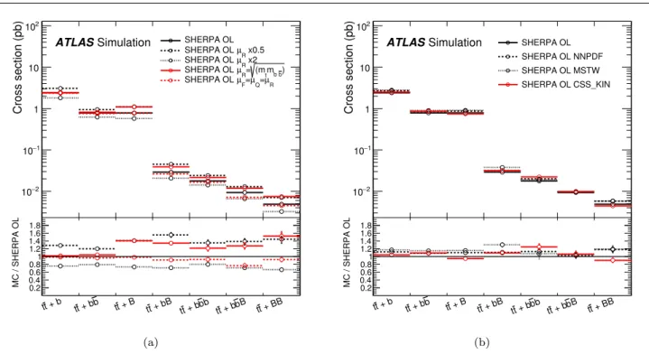
Arbitrary units 3 − 10 2 − 10 1 − 10 1

10 ATLAS Simulation _{POWHEG+PYTHIA}

MADGRAPH+PYTHIA SHERPA OL + b t t tt + bbtt + Btt + bBtt + bbtbt + bbBtt + BB_t_{+ FSR B} t tt + MPI btt + FSR BB b + MPI b t t MC / POWHEG+PYTHIA 0.2 0.4 0.6 0.81 1.2 1.4 1.6 1.8

Fig. 4 Relative contributions of different categories of t¯t+b¯b events in Powheg+Pythia, Madgraph+Pythia and Sher-paOL samples. Labels “t¯t+MPI” and “t¯t+FSR” refer to events where heavy flavour is produced via multiparton in-teraction (MPI) or final state radiation (FSR), respectively. These contributions are not included in the SherpaOL cal-culation. An arrow indicates that the point is off-scale. Un-certainties are from the limited MC sample sizes.

The relative distribution across categories is such

that SherpaOL predicts a higher contribution of the

t¯

t+B category, as well as every category where the

pro-duction of a second b¯

b pair is required. The modelling of

the relevant kinematic variables in each category is in

reasonable agreement between Powheg+Pythia and

SherpaOL. Some differences are observed in the very

low regions of the mass and p

T

of the b¯

b pair, and in

the p

T

of the top quark and t¯

t systems.

The prediction from SherpaOL is expected to model

the t¯

t + b¯

b contribution more accurately than both

Powheg+Pythia and Madgraph+Pythia. Thus, in

(8)

the analysis t¯

t+b¯

_{b events are reweighted from Powheg+}

Pythia to reproduce the NLO t¯

t+b¯

b prediction from

SherpaOL for relative contributions of different

cat-egories as well as their kinematics. The reweighting is

done at generator level using several kinematic

vari-ables such as the top quark p

T

, t¯

t system p

T

, ∆R and

p

T

of the dijet system not coming from the top quark

decay. In the absence of an NLO calculation of t¯

t+c¯

c

production, the Madgraph+Pythia sample is used

to evaluate systematic uncertainties on the t¯

t+c¯

c

back-ground.

Since achieving the best possible modelling of the

t¯

t+jets background is a key aspect of this analysis, a

separate reweighting is applied to t¯

t+light and t¯

t+c¯

c

events in Powheg+Pythia based on the ratio of

mea-sured differential cross sections at

√

s = 7 TeV in data

and simulation as a function of top quark p

T

and t¯

t

system p

T

[57]. It was verified using the simulation

that the ratio derived at

√

s = 7 TeV is applicable

to

√

s = 8 TeV simulation. It is not applied to the

t¯

t+b¯

b component since that component was corrected

to match the best available theory calculation.

More-over, the measured differential cross section is not

sen-sitive to this component. The reweighting significantly

improves the agreement between simulation and data

in the total number of jets (primarily due to the t¯

t

sys-tem p

T

reweighting) and jet p

T

(primarily due to the

top quark p

T

reweighting). This can be seen in Fig. 5,

where the number of jets and the scalar sum of the jet

p

T

(H

Thad

) distributions in the exclusive 2-b-tag region

are plotted in the single-lepton channel before and after

the reweighting is applied.

5.2 Other backgrounds

The W/Z+jets background is estimated from

simula-tion reweighted to account for the difference in the W/Z

p

T

spectrum between data and simulation [58]. The

heavy-flavour fraction of these simulated backgrounds,

i.e. the sum of W/Z+b¯

b and W/Z+c¯

c processes, is

ad-justed to reproduce the relative rates of Z events with

no b-tags and those with one b-tag observed in data.

Samples of W/Z+jets events, and diboson production

in association with jets, are generated using the

Alp-gen 2.14 [59] leading-order (LO) Alp-generator and the

CTEQ6L1 PDF set. Parton showers and

fragmenta-tion are modelled with Pythia 6.425 for W/Z+jets

production and with Herwig 6.520 [60] for diboson

production. The W +jets samples are generated with

up to five additional partons, separately for W

+light-jets, W b¯

b+jets, W c¯

c+jets, and W c+jets. Similarly, the

Z+jets background is generated with up to five

addi-tional partons separated in different parton flavours.

Both are normalised to the respective inclusive NNLO

theoretical cross section [61]. The overlap between W Q ¯

Q

(ZQ ¯

Q)(Q = b, c) events generated from the matrix

el-ement calculation and those from parton-shower

evo-lution in the W +light-jet (Z+light-jet) samples is

re-moved by an algorithm based on the angular separation

between the extra heavy quarks: if ∆R(Q, ¯

Q) > 0.4, the

matrix element prediction is used, otherwise the parton

shower prediction is used.

The diboson+jets samples are generated with up to

three additional partons and are normalised to their

respecitve NLO theoretical cross sections [62].

Samples of single top quark backgrounds are

gen-erated with Powheg-Box 2.0 using the CT10 PDF

set. The samples are interfaced to Pythia 6.425 with

the CTEQ6L1 set of parton distribution functions and

Perugia2011C underlying-event tune. Overlaps between

the t¯

t and W t final states are removed [63]. The

sin-gle top quark samples are normalised to the

approxi-mate NNLO theoretical cross sections [64–66] using the

MSTW2008 NNLO PDF set [67, 68].

Samples of t¯

_{t + V are generated with Madgraph}

5 and the CTEQ6L1 PDF set. Pythia 6.425 with the

AUET2B tune [69] is used for showering. The t¯

tV

sam-ples are normalised to the NLO cross-section

predic-tions [70, 71].

5.3 Signal model

The t¯

tH signal process is modelled using NLO

ma-trix elements obtained from the HELAC-Oneloop

pack-age [72]. Powheg-Box serves as an interface to shower

Monte Carlo programs. The samples created using this

approach are referred to as PowHel samples [73]. They

are inclusive in Higgs boson decays and are produced

using the CT10nlo PDF set and factorisation (µ

F

) and

renormalisation scales set to µ

F

= µ

R

= m

t

+ m

H

/2.

The PowHel t¯tH sample is showered with Pythia

8.1 [74] with the CTEQ6L1 PDF and the AU2

underlying-event tune [75]. The t¯

tH cross section and Higgs boson

decay branching fractions are taken from (N)NLO

the-oretical calculations [19, 76–82], collected in Ref. [83].

In Appendix A, the relative contributions of the Higgs

boson decay modes are shown for all regions considered

in the analysis.

5.4 Common treatment of MC samples

All samples using Herwig are also interfaced to Jimmy

4.31 [84] to simulate the underlying event. All simulated

samples utilise Photos 2.15 [85] to simulate photon

radiation and Tauola 1.20 [86] to simulate τ decays.

(9)

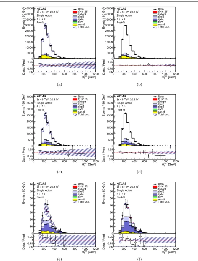
Events 0 20 40 60 80 100 120 140 3 10 × Data H (125) t t +light t t c +c t t b +b t t +V t t t non-t Total unc. ATLAS -1 = 8 TeV, 20.3 fb s 4 j, 2 b ≥ Single lepton Before reweighting Njets 3 4 5 6 7 8 9 Data / Pred 0.5 0.75 1 1.25 1.5 0 (a) Events 0 20 40 60 80 100 120 140 3 10 × Data H (125) t t +light t t c +c t t b +b t t +V t t t non-t Total unc. ATLAS -1 = 8 TeV, 20.3 fb s 4 j, 2 b ≥ Single lepton After reweighting Njets 3 4 5 6 7 8 9 Data / Pred 0.5 0.75 1 1.25 1.5 0 (b) Events / 50 GeV 10 2 10 3 10 4 10 5 10 6 10 Data H (125) t t +light t t c +c t t b +b t t +V t t t non-t Total unc. ATLAS -1 = 8 TeV, 20.3 fb s 4 j, 2 b Single lepton Before reweighting [GeV] had T H 200 400 600 800 1000 1200 Data / Pred 0.5 0.75 1 1.25 1.5 (c) Events / 50 GeV 10 2 10 3 10 4 10 5 10 6 10 Data H (125) t t +light t t c +c t t b +b t t +V t t t non-t Total unc. ATLAS -1 = 8 TeV, 20.3 fb s 4 j, 2 b Single lepton After reweighting [GeV] had T H 200 400 600 800 1000 1200 Data / Pred 0.5 0.75 1 1.25 1.5 (d)

Fig. 5 The exclusive 2-b-tag region of the single-lepton channel before and after the reweighting of the pTof the t¯t system

and the pTof the top quark of the Powheg+Pythia t¯t sample. The jet multiplicity distribution (a) before and (b) after the

reweighting; Hhad

T distributions (c) before and (d) after the reweighting.

Events from minimum-bias interactions are simulated

with the Pythia 8.1 generator with the MSTW2008

LO PDF set and the AUET2 [87] tune. They are

su-perimposed on the simulated MC events, matching the

luminosity profile of the recorded data. The

contribu-tions from these pileup interaccontribu-tions are simulated both

within the same bunch crossing as the hard-scattering

process and in neighbouring bunch crossings.

Finally, all simulated MC samples are processed

thr-ough a simulation [88] of the detector geometry and

response either using Geant4 [89], or through a fast

simulation of the calorimeter response [90]. All

simu-lated MC samples are processed through the same

re-construction software as the data. Simulated MC events

are corrected so that the object identification

efficien-cies, energy scales and energy resolutions match those

determined from data control samples.

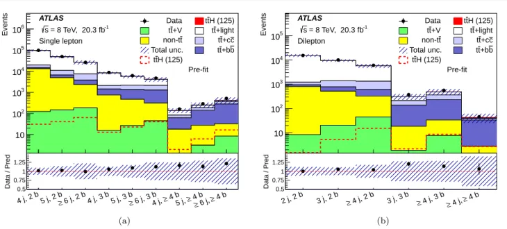
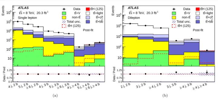
Figures 6(a) and 6(b) show a comparison of

pre-dicted yields to data prior to the fit described in Sect. 9

in all analysis regions in the single-lepton and dilepton

channel, respectively. The data agree with the SM

ex-pectation within the uncertainties of 10-30 %. Detailed

tables of the event yields prior to the fit and the

cor-responding S/B and S/

√

B ratios for the single-lepton

and dilepton channels can be found in Appendix B.

When requiring high jet and b-tag multiplicity in the

analysis, the number of available MC events is

signifi-cantly reduced, leading to large fluctuations in the

re-sulting distributions for certain samples. This can

neg-atively affect the sensitivity of the analysis through the

(10)

4 j, 2 b 4 j, 3 b 4 j, ≥ 4 b 5 j, 2 b 5 j, 3 b 5 j, ≥ 4 b ≥ 6 j, 2 b ≥ 6 j, 3 b ≥ 6 j, ≥ 4 b Events 10 2 10 3 10 4 10 5 10 6 10 Data ttH (125) +V t t tt+light t non-t tt+cc Total unc. tt+bb H (125) t t ATLAS -1 = 8 TeV, 20.3 fb s Pre-fit Single lepton 4 j, 2 b 5 j, 2 b 6 j, 2 b≥ 4 j, 3 b 5 j, 3 b 6 j, 3 b≥ 4 j, ≥ 4 b5 j, ≥ 4 b_≥ 6 j, ≥ 4 b Data / Pred 0.5 0.75 1 1.25 1.5 (a) 2 j, 2 b 3 j, 2 b 3 j, 3 b ≥ 4 j, 2 b ≥ 4 j, 3 b ≥ 4 j, ≥ 4 b Events 10 2 10 3 10 4 10 5 10 Data ttH (125) +V t t tt+light t non-t tt+cc Total unc. tt+bb H (125) t t ATLAS -1 = 8 TeV, 20.3 fb s Pre-fit Dilepton 2 j, 2 b 3 j, 2 b ≥ 4 j, 2 b 3 j, 3 b ≥ 4 j, 3 b_≥ 4 j, ≥ 4 b Data / Pred 0.5 0.75 1 1.25 1.5 (b)

Fig. 6 Comparison of prediction to data in all analysis regions before the fit to data in (a) the single-lepton channel and (b) the dilepton channel. The signal, normalised to the SM prediction, is shown both as a filled red area stacked on the backgrounds and separately as a dashed red line. The hashed area corresponds to the total uncertainty on the yields.

large statistical uncertainties on the templates and

un-reliable systematic uncertainties due to shape

fluctua-tions. In order to mitigate this problem, instead of

tag-ging the jets by applying the b-tagtag-ging algorithm, their

probabilities to be b-tagged are parameterised as

func-tions of jet flavour, p

T

, and η. This allows all events in

the sample before b-tagging is applied to be used in

pre-dicting the normalisation and shape after b-tagging [91].

The tagging probabilities are derived using an inclusive

t¯

t+jets simulated sample. Since the b-tagging

probabil-ity for a b-jet coming from top quark decay is slightly

higher than that of a b-jet with the same p

T

and η but

arising from other sources, they are derived separately.

The predictions agree well with the normalisation and

shape obtained by applying the b-tagging algorithm

di-rectly. The method is applied to all signal and

back-ground samples.

6 Analysis method

In both the single-lepton and dilepton channels, the

analysis uses a neural network (NN) to discriminate

signal from background in each of the regions with

significant expected t¯

tH signal contribution since the

S/

√

B is very small and the uncertainty on the

back-ground is larger than the signal. Those include (5j, ≥

4b), (≥ 6j, 3b) and (≥ 6j, ≥ 4b) in the case of the

single-lepton channel, and (≥ 4j, 3b) and (≥ 4j, ≥ 4b) in the

case of the dilepton channel. In the dilepton channel,

an additional NN is used to separate signal from

back-ground in the (3j, 3b) channel. Despite a small expected

S/

√

B, it nevertheless adds sensitivity to the signal due

to a relatively high expected S/B. In the single-lepton

channel, a dedicated NN is used in the (5j, 3b) region to

separate t¯

t+light from t¯

t+HF backgrounds. The other

regions considered in the analysis have lower

sensitiv-ity, and use H

had

T

in the single-lepton channel, and the

scalar sum of the jet and lepton p

T

(H

T

) in the dilepton

channel as a discriminant.

The NNs used in the analysis are built using the

NeuroBayes [92] package. The choice of the variables

that enter the NN discriminant is made through the

ranking procedure implemented in this package based

on the statistical separation power and the correlation

of variables. Several classes of variables were

consid-ered: object kinematics, global event variables, event

shape variables and object pair properties. In the

re-gions with ≥ 6 (≥ 4) jets, a maximum of seven (five)

jets are considered to construct the kinematic variables

in the single-lepton (dilepton) channel, first using all the

b-jets, and then incorporating the untagged jets with

the highest p

T

. All variables used for the NN training

and their pairwise correlations are required to be

de-scribed well in simulation in multiple control regions.

In the (5j, 3b) region in the single-lepton channel,

the separation between the t¯

t+light and t¯

t+HF events

is achieved by exploiting the different origin of the third

b-jet in the case of t¯

t+light compared to t¯

t+HF events.

In both cases, two of the b-jets originate from the t¯

t

decay. However, in the case of t¯

t+HF events, the third

b-jet is likely to originate from one of the additional

(11)

heavy-flavour quarks, whereas in the case of t¯

t+light

events, the third b-jet is often matched to a c-quark

from the hadronically decaying W boson. Thus,

kine-matic variables, such as the invariant mass of the two

untagged jets with minimum ∆R, provide

discrimina-tion between t¯

t+light and t¯

t+HF events, since the

lat-ter presents a distinct peak at the W boson mass which

is not present in the former. This and other kinematic

variables are used in the dedicated NN used in this

re-gion.

In addition to the kinematic variables, two variables

calculated using the matrix element method (MEM),

detailed in Sect. 7, are included in the NN training in

(≥ 6j, 3b) and (≥ 6j, ≥ 4b) regions of the single-lepton

channel. These two variables are the Neyman–Pearson

likelihood ratio (D1) (Eq. (4)) and the logarithm of

the summed signal likelihoods (SSLL) (Eq. (2)). The

D1 variable provides the best separation between t¯

tH

signal and the dominant t¯

t+b¯

b background in the

(≥ 6j, ≥ 4b) region. The SSLL variable further improves

the NN performance.

The variables used in the single-lepton and dilepton

channels, as well as their ranking in each analysis

re-gion, are listed in Tables 1 and 2, respectively. For the

construction of variables in the (≥ 4j, ≥ 4b) region of

the dilepton channel, the two b-jets that are closest in

∆R to the leptons are considered to originate from the

top quarks, and the other two b-jets are assigned to the

Higgs candidate.

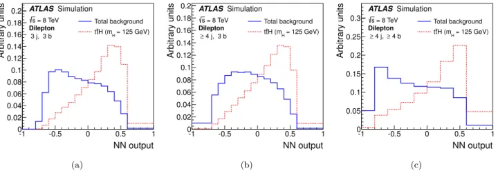
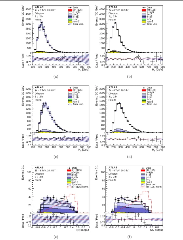
Figures 7 and 8 show the distribution of the NN

discriminant for the t¯

tH signal and background in the

single-lepton and dilepton channels, respectively, in the

signal-rich regions. In particular, Fig. 7(a) shows the

separation between the t¯

t+HF and t¯

t+light-jet

produc-tion achieved by a dedicated NN in the (5j, 3b) region

in the single-lepton channel. The distributions in the

highest-ranked input variables from each of the NN

re-gions are shown in Appendix C.

For all analysis regions considered in the fit, the t¯

tH

signal includes all Higgs decay modes. They are also

included in the NN training.

The analysis regions have different contributions from

various systematic uncertainties, allowing the combined

fit to constrain them. The highly populated (4j, 2b) and

(2j, 2b) regions in the single-lepton and dilepton

chan-nels, respectively, provide a powerful constraint on the

overall normalisation of the t¯

t background. The (4j, 2b),

(5j, 2b) and (≥ 6j, 2b) regions in the single-lepton

chan-nel and the (2j, 2b), (3j, 2b) and (≥ 4j, 2b) regions in

the dilepton channel are almost pure in t¯

t+light-jets

background and provide an important constraint on t¯

t

modelling uncertainties both in terms of normalisation

and shape. Uncertainties on c-tagging are reduced by

exploiting the large contribution of W → cs decays

in the t¯

t+light-jets background populating the (4j, 3b)

region in the single-lepton channel. Finally, the

consid-eration of regions with exactly 3 and ≥ 4 b-jets in both

channels, having different fractions of t¯

t+b¯

b and t¯

t+c¯

c

backgrounds, provides the ability to constrain

uncer-tainties on the t¯

t+b¯

b and t¯

t+c¯

c normalisations.

7 The matrix element method

The matrix element method [94] has been used by the

D0 and CDF collaborations for precision measurements

of the top quark mass [95,96] and for the observations of

single top quark production [97,98]. Recently this

tech-nique has been used for the t¯

tH search by the CMS

experiment [99]. By directly linking theoretical

calcula-tions and observed quantities, it makes the most

com-plete use of the kinematic information of a given event.

The method calculates the probability density

func-tion of an observed event to be consistent with physics

process i described by a set of parameters α. This

prob-ability density function P

i

(x|α) is defined as

P

i

(x|α) =

(2π)

4

σ

_iexp

(α)

Z

dp

A

dp

B

f (p

A

) f (p

B

)

|M

i

(y|α)|

2

F

W (y|x) dΦ

N

(y)

(1)

and is obtained by numerical integration over the entire

phase space of the initial- and final-state particles. In

this equation, x and y represent the four-momentum

vectors of all final-state particles at reconstruction and

parton level, respectively. The flux factor F and the

Lorentz-invariant phase space element dΦ

N

describe

the kinematics of the process. The transition matrix

element M

i

is defined by the Feynman diagrams of the

hard process. The transfer functions W (y|x) map the

detector quantities x to the parton level quantities y.

Finally, the cross section σ

exp_i

normalises P

i

to unity

taking acceptance and efficiency into account.

The assignment of reconstructed objects to

final-state partons in the hard process contains multiple

am-biguities. The process probability density is calculated

for each allowed assignment permutation of the jets to

the final-state quarks of the hard process. A process

likelihood function can then be built by summing the

process probabilities for the N

p

allowed assignment

per-mutation,

L

i

(x|α) =

Np

X

p=1

P

_ip

(x|α) .

(2)

(12)

Variable

Definition

NN rank

≥ 6j, ≥ 4b

≥ 6j, 3b

5j, ≥ 4b

5j, 3b

D1

Neyman–Pearson MEM discriminant (Eq. (4))

1

10 -

-Centrality

Scalar sum of the p

_{all jets and the lepton}

T

divided by sum of the E for

2

1 -p

jet5_T

p

T

of the fifth leading jet

3

7 -

-H1

Second Fox–Wolfram moment computed using

_{all jets and the lepton}

4

3

2 -∆R

avg_bb

Average ∆R for all b-tagged jet pairs

5

6

5 -SSLL

Logarithm of the summed signal likelihoods (Eq. (2))

6

4 -

-m

min ∆R_bb

Mass of the combination of the two b-tagged

_{jets with the smallest ∆R}

7

12

4

4 m

max pT

bj

Mass of the combination of a b-tagged jet and

8

8 -

-any jet with the largest vector sum p

T

∆R

max pT

bb

∆R between the two b-tagged jets with the

9 -

-

-largest vector sum p

T

∆R

min ∆R_lep−bb

∆R between the lepton and the combination

_{of the two b-tagged jets with the smallest ∆R}

10

11

10 -m

min ∆R

uu

Mass of the combination of the two untagged jets

11

9 -

2 with the smallest ∆R

Aplan

b−jet

1.5λ

2

, where λ

2

is the second eigenvalue of the

12 -

8 -momentum tensor [93] built with only b-tagged jets

N

₄₀jet

Number of jets with p

T

≥ 40 GeV

-

1

3 -m

min ∆R_bj

Mass of the combination of a b-tagged jet and

_{any jet with the smallest ∆R}

-

5 -

-m

max pT

jj

Mass of the combination of any two jets with

-

6 -the largest vector sum p

T

H

had

T

Scalar sum of jet p

T

-

7 -m

min ∆R_jj

Mass of the combination of any two jets with

_{the smallest ∆R}

-

9 -m

max pT

bb

Mass of the combination of the two b-tagged

-

1 jets with the largest vector sum p

T

p

min ∆R

T,uu

Scalar sum of the p

T

of the pair of untagged

-

3 jets with the smallest ∆R

m

max m

bb

Mass of the combination of the two b-tagged

-

5 jets with the largest invariant mass

∆R

min ∆R

uu

Minimum ∆R between the two untagged jets

-

6 m

jjj

Mass of the jet triplet with the largest vector

-

7 sum p

T

Table 1 Single-lepton channel: the definitions and rankings of the variables considered in each of the regions where an NN is used.

The process probability densities are used to

distin-guish signal from background events by calculating the

likelihood ratio of the signal and background processes

contributing with fractions f

bkg

,

r

sig

(x|α) =

L

sig

(x|α)

P

bkg

f

bkg

L

bkg

(x|α)

.

(3)

This ratio, according to the Neyman–Pearson

lem-ma [100], is the most powerful discriminant between

signal and background processes. In the analysis, this

variable is used as input to the NN along with other

kinematic variables.

Matrix element calculation methods are generated

with Madgraph 5 in LO. The transfer functions are

obtained from simulation following a similar procedure

as described in Ref. [101]. For the modelling of the

par-ton distribution functions the CTEQ6L1 set from the

LHAPDF package [102] is used.

The integration is performed using VEGAS [103].

Due to the complexity and high dimensionality,

adap-tive MC techniques [104], simplifications and

approxi-mations are needed to obtain results within a

reason-able computing time. In particular, only the

numeri-cally most significant contributing helicity states of a

process hypothesis for a given event, identified at the

(13)

Variable

Definition

NN rank

≥ 4j, ≥ 4b

≥ 4j, 3b

3j, 3b

∆η

max ∆η_jj

Maximum ∆η between any two jets in the event

1

1 m

min ∆R_bb

Mass of the combination of the two b-tagged jets with

_{the smallest ∆R}

2

8 -m

b¯b

Mass of the two b-tagged jets from the Higgs candidate

3 -

-system

∆R

min ∆R

hl

∆R between the Higgs candidate and the closest lepton

4

5 -N

Higgs₃₀

Number of Higgs candidates within 30 GeV of the Higgs

_{mass of 125 GeV}

5

2

5 ∆R

max pT

bb

∆R between the two b-tagged jets with the largest

6

4

8 vector sum p

T

Aplan

jet

1.5λ

2

, where λ

2

is the second eigenvalue of the

7

7 -momentum tensor built with all jets

m

min m

jj

Minimum dijet mass between any two jets

8

3

2 ∆R

_hlmax ∆R

∆R between the Higgs candidate and the furthest lepton

9 -

-m

closest

jj

Dijet mass between any two jets closest to the Higgs

10 -

10 mass of 125 GeV

H

T

Scalar sum of jet p

T

and lepton p

T

values

-

6

3 ∆R

max m

bb

∆R between the two b-tagged jets with the largest

-

9 -invariant mass

∆R

min ∆R

lj

Minimum ∆R between any lepton and jet

-

10 -Centrality

Sum of the p

_{both leptons}

T

divided by sum of the E for all jets and

-

7 m

max pT

jj

Mass of the combination of any two jets with the largest

-

9 vector sum p

T

H4

Fifth Fox–Wolfram moment computed using all jets and

_{both leptons}

-

4 p

jet3_T

p

T

of the third leading jet

-

6

Table 2 Dilepton channel: the definitions and rankings of the variables considered in each of the regions where an NN is used.

start of each integration, are evaluated. This does not

perceptibly decrease the separation power but reduces

the calculation time by more than an order of

magni-tude. Furthermore, several approximations are made to

improve the VEGAS convergence rate. Firstly, the

di-mensionality of integration is reduced by assuming that

the final-state object directions in η and φ as well as

charged lepton momenta are well measured, and

there-fore the corresponding transfer functions are represented

by δ functions. The total momentum conservation and

a negligible transverse momentum of the initial-state

partons allow for further reduction. Secondly, kinematic

transformations are utilised to optimise the integration

over the remaining phase space by aligning the peaks

of the integrand with the integration dimensions. The

narrow-width approximation is applied to the

leptoni-cally decaying W boson. This leaves three b-quark

en-ergies, one light-quark energy, the hadronically

decay-ing W boson mass and the invariant mass of the two

b-quarks originating from either the Higgs boson for

the signal or a gluon for the background as the

re-maining parameters which define the integration phase

space. The total integration volume is restricted based

upon the observed values and the width of the

trans-fer functions and of the propagator peaks in the matrix

elements. Finally, the likelihood contributions of all

al-lowed assignment permutations are coarsely integrated,

and only for the leading twelve assignment

permuta-tions is the full integration performed, with a required

precision decreasing according to their relative

contri-butions.

The signal hypothesis is defined as a SM Higgs

bo-son produced in association with a top-quark pair as

shown in Fig. 1(a), (b). Hence no coupling of the Higgs

boson to the W boson is accounted for in |M

i

|

2

to

allow for a consistent treatment when performing the

kinematic transformation. The Higgs boson is required

to decay into a pair of b-quarks, while the top-quark

pair decays into the single-lepton channel. For the

back-ground hypothesis, only the diagrams of the irreducible

t¯

t + b¯

b background are considered. Since it dominates

the most signal-rich analysis regions, inclusion of other

processes does not improve the separation between

sig-nal and background. No gluon radiation from the fisig-nal-

(14)

final-NN output 1 − −0.5 0 0.5 1 Arbitrary units 0 0.02 0.04 0.06 0.08 0.1 0.12 0.14 0.16 +light t t +HF t t 5 j, 3 b Single lepton = 8 TeV s ATLAS Simulation (a) NN output 1 − −0.5 0 0.5 1 Arbitrary units 0 0.02 0.04 0.06 0.08 0.1 0.12 0.14 0.16 0.18 0.2 Total background = 125 GeV) H H (m t t 4 b ≥ 5 j, Single lepton = 8 TeV s ATLAS Simulation (b) NN output 1 − −0.5 0 0.5 1 Arbitrary units 0 0.01 0.02 0.03 0.04 0.05 0.06 0.07 0.08 Total background = 125 GeV) H H (m t t 6 j, 3 b ≥ Single lepton = 8 TeV s ATLAS Simulation (c) NN output 1 − −0.5 0 0.5 1 Arbitrary units 0 0.02 0.04 0.06 0.08 0.1 0.12 0.14 0.16 0.18 Total background = 125 GeV) H H (m t t 4 b ≥ 6 j, ≥ Single lepton = 8 TeV s ATLAS Simulation (d)

Fig. 7 Single-lepton channel: NN output for the different regions. In the (5j, 3b) region (a), the t¯t+HF production is considered as signal and t¯t+light as background whereas in the (5j, ≥ 4b) (b), (≥ 6j, 3b) (c), and (≥ 6j, ≥ 4b) (d) regions the NN output is for the t¯tH signal and total background. The distributions are normalised to unit area.

NN output -1 -0.5 0 0.5 1 Arbitrary units 0 0.02 0.04 0.06 0.08 0.1 0.12 0.14 0.16 0.18 0.2 ATLAS Simulation = 8 TeV s Dilepton 3 j, 3 b Total background = 125 GeV) H H (m t t (a) NN output -1 -0.5 0 0.5 1 Arbitrary units 0 0.02 0.04 0.06 0.08 0.1 0.12 0.14 0.16 0.18 0.2 _{ATLAS Simulation} = 8 TeV s Dilepton 4 j, 3 b ≥ Total background = 125 GeV) H H (m t t (b) NN output -1 -0.5 0 0.5 1 Arbitrary units 0 0.05 0.1 0.15 0.2 0.25 0.3 ATLAS Simulation = 8 TeV s Dilepton 4 b ≥ 4 j, ≥ Total background = 125 GeV) H H (m t t (c)

Fig. 8 Dilepton channel: NN output for the t¯tH signal and total background in the (a) (3j, 3b), (b) (≥ 4j, 3b), and (c) (≥ 4j, ≥ 4b) regions. The distributions are normalised to unit area.