A Work Project, presented as part of the requirements for the Award of a Masters Degree in Finance from NOVA School of Business and Economics
POST EARNINGS ANNOUNCEMENT DRIFT IN PSI20
RUI DIOGO MARTINS
30002
A Project carried out with the supervision of
Pedro Lameira
2 ABSTRACT
This paper presents an innovative application of post-earnings announcement drift in the PSI-20 from 2011-2017. We show that abnormal returns exist, and are more significant when we incorporate momentum and liquidity factors for different earnings surprises. Moreover, we implement an investment strategy, including transaction costs, which takes advantage of such abnormal returns. A hedging strategy designed according to the stock’s proximity to 52-week high and earnings surprise yields an info Sharpe of 1.78 and a 65.12% accuracy. Finally, we show that a long-portfolio on PSI-20 equities with a 20-day holding period presents unsatisfactory results when incorporating transaction costs.
Keywords: Post-earnings Announcement Drift, 52-week high, Earnings Surprise, Liquidity
Acknowledgments
I am grateful to my supervisor, Pedro Lameira, for all the recommendations, enthusiasm and suggestions. I am also utterly thankful to my friend Francisco Veiga for being a truthful mentor throughout my academic life in Finance.
3
I. Introduction
Over the past few years, research papers on post-earnings announcement drift1 (henceforth
PEAD) have often relied on US and the most liquid European equity markets (France, Germany, Spain and United Kingdom). Current literature available2 regarding capital markets reaction to
earnings announcements in PSI-203 is not substantial to fully comprehend the subject, making
further investigation very attractive. Portuguese stock market analysis also brings a further advantage grounded in its low liquidity and poor financial information quality when compared to other European markets. Most of these attempts to statistically prove abnormal returns tend to forget the investment side of the research. Additionally, research papers in PSI-20 do not exist after 2009 financial crisis.
This paper departs from previous research on PEAD in three ways. First, we focus in the Portuguese stock market, with a lower liquidity when compared to other European and US markets. Second, we observe a post-crisis period 4 that might have incorporated a new risk aversion factor
that could bear for the following decade. This paper examines whether PEAD abnormal returns are just attributable to a given sub-period or profitable over time. Third, we develop, when applicable, a trading strategy according to stock’s liquidity and momentum for different earnings surprise (positive, negative and no surprise). One of the main objectives of implementing such strategy is to observe whether an event-study method would overestimate abnormal returns since it does not incorporate transaction costs. This paper pretends to observe if profits continue to exist after implementing such strategies or if transaction costs eliminate that abnormal gain. Therefore, the
1 PEAD is the tendency for a stock’s cumulative abnormal return to drift in the direction of an earnings surprise for a given time period following the announcement.
2 Wilton (2002), Alves and Santos (2005), Duque and Pinto (2005), Romacho and Cidrais (2007), Lourenço and Coelho (2008). 3 PSI-20 is the reference Portuguese stock index and aggregates the 20 largest (nowadays, are just 18 companies) Portuguese companies trading in Euronext Lisbon.
4 main objective here is to substantiate if there are abnormal returns surrounding earnings announcement dates in PSI 20 from 2011-2015. If true, test the feasibility of such a model by implementing an Equity-Long Only and Equity Long-Short strategies from 2015-2017.
II. Literature Review
Contradictory views about PEAD are very common in authors trying to explore this subject, enhancing the pace at which ideas are changing. Take for example Fama (1970) which pointed out that capital markets are efficient if security prices, at any given time, fully reflect all available information and hence the impossibility of generating abnormal returns. Nevertheless, Fama (1998) reported that post-earnings announcement drift is a robust and persistent anomaly that goes against market semi-strong efficiency form and that occurs mainly in highly illiquid stocks. Post-earnings announcement drift is reported by many authors to represent a market anomaly. Ball and Brown (1968) were the first to notice that stock prices tended to drift upwards (downwards) after earnings announcements if the surprise is positive (negative). Of course, this constitutes a clear violation of the market efficiency hypothesis if one shows that abnormal returns are statistically significant. Authors like Beaver (1968) noticed that both trading activity and price volatility increased during the week surrounding earnings announcements meaning that earnings information brings additional value to the stock market. Posteriorly, May (1971) also noticed that price changes during the weeks of quarterly earnings announcements were, in fact, higher when compared to the average price change. Joy et al. (1977) showed that unanticipated favorable quarterly earnings announcements showed a statistically significant relationship with abnormal price changes over the subsequent 26 weeks. The new information released about an equity’s fundamental or intrinsic value origins an intermediate stock price trend (Jones and Litzenberger, 1970). They confirmed that oscillations in the market’s general belief relative to the stock’s intrinsic value may cause price
5 corrections over time. These price adjustments are steady since those beliefs need to be gradually assimilated by investors and consequently increase stock’s momentum and attractiveness. A surprise in EPS reported by the firm (considering historical earnings trend) is estimated to cause positive revisions in the fundamental value of a given stock. Hence, creating positive price adjustments over time. The opposite rationale for earnings below expected is also valid.5 In a
similar study, Bernard and Thomas (1989) determined that PEAD is consistent with a deferred response rather than a risk mismeasurement.6 In fact, decades later Chudek et al. (2011) and Truong
(2010, 2011) concluded that PEAD is caused by a delayed assimilation of earnings information by the investors in the Canadian, New Zealand and Chinese equity market, respectively. Ball and Shivakumar (2008) also pointed out that earnings announcements convey relevant and essential market information since they seem to generate some market response. Their main results showed that the average quarterly earnings announcement is usually associated with abnormal price volatility.
Shifting our focus to the European markets, Forner et al. (2009) reported that PEAD long-short strategies yield significant positive returns in the months after the earnings announcement in Spanish stock market, and make “things more difficult for the market efficiency hypothesis.” Liu et al. (2000) found significant evidence that suggests a drift in returns after earnings announcements by companies in the United Kingdom, and that market risk, size, book-to-market, price, cash earnings-to-price and number of analysts failed to explain PEAD phenomenon. The variable that better explained PEAD effect was the four-day return around earnings announcement. They showed that PEAD constituted a “clear rejection of the efficient market hypothesis” and that
5 They analyzed two samples of stocks, with 510 companies in the first sample covering a period since 1962-1965. The second sample during the years 1964-1967 for 618 companies. Represents all the companies available from Quarterly Compustat tapes. 6 Their sample included 84 792 firm-quarters of data for NYSE/AMEX firms between 1974 and 1986. They also performed additional tests on 15 457 firm-quarters of data for OTC stocks on the NASDAQ, in the period 1974-85.
6 investors failed to process earnings information efficiently. Forbes and Giannopoulos (2015) confirmed the existence of PEAD anomaly in the Greek market, and state that it increased after the adoption of the international financial reporting standards. On the other hand, Wael (2004) reported that abnormal returns dissipate within the first fifteen minutes in the Euronext Paris, though he emphasizes the fact that there are information asymmetry and bid-ask spread increases just after disclosing earnings information. Regarding the Portuguese Stock Market, some authors stand out. Wilton (2002), Pinto (2005) and Romacho et al. (2007) stated that, for the generality of the set of stocks, the market was efficient and therefore it was not possible to obtain abnormal profits. Nonetheless, Lourenço and Coelho (2008) argued that annual earnings announcements are strongly correlated with stock’s abnormal returns. Furthermore, Alves and Santos (2005) showed that the results obtained in their study indicate that earnings reporting had a significant impact on the 3, 5 and 7 trading days following the announcement, resulting in abnormal price volatility and volume.
As described, a substantial amount of literature presents that abnormal returns exist and that PEAD sustains in the medium/long term in US, Asia and Europe. Nonetheless, one must ensure if it is due to earnings specific information or if there are other variables that might influence the outcome. In fact, Santa-Clara et al. (2008) hypothesized that a significant share of the market reaction around the announcement date is attributable to non-earnings information. Following this general idea, one will consider how liquidity and momentum explain PEAD in stocks with positive, negative or no earnings surprise. Consensus does not exist among authors regarding PEAD and its correlation with earnings surprise. Chen et al. (2015) showed that there is a stronger positive pattern in price movement and that it persists for up to 250 days after the announcement in stocks that had
7 a positive surprise. On the other hand, Schmitz (2007) observed exactly the opposite, where he finds a larger drift for stock with bad news and a very short-term price drift for positive news. 7
PEAD drift is witnessed mainly in highly illiquid stocks. Chordia (2009), using cross-sectional asset pricing tests, presented that the level of liquidity has an impact on the drift. Company size also affects the drift, however this effect could occur because size is a proxy for liquidity. 8 There
is a correlation between liquidity and the amount of information available in the market, for every equity. Chen et al. (1997) attributed earnings surprise (positive, negative or neutral) and stock price drift to be more substantial when there is less quality and quantity of information. Portuguese stock market has fewer equity analysts tracking stocks and therefore exists a poor quantity/quality of available information.9Another variable that might influence the event-study results is momentum.
The way investors’ trade stocks on earnings may depend on stock’s past performance. Goh and Jeon (2017) used 52-week as a proxy for momentum and concluded that stocks with positive (negative) earnings news do not experience a positive (negative) drift when stock prices are far (near) 52-week high. They used anchoring bias10 to explain PEAD in Korean stock market.
III. Methodology
A. Estimation and Event Window
Due to the main purpose of this paper, we will only focus on quarterly earnings announcements, which are mandatory in Portugal. 11 Earnings announcement dates will be considered as the date
in which there exists the first formal communication to the stock market. Let us define day 0 as the
7 Note that both studies are performed in different countries: China and Germany. Thus, this could be a possible explanation for such different study conclusions’. The main idea here is that opinions about the same subject differ among the authors.
8 Sample analyzed was composed of all NYSE and Amex companies between January 1972 and December 2005.
9 Analysts tracking Portuguese stocks are very few. In fact, half of PSI-20 stocks do not have specific analysts following the stocks (this results for example, in no forecasted EPS or lack of market consensus regarding a stock’s target price). The others (most liquid ones) only have up to four analysts tracking them. Hence, making statistical inference and market analysis not significant. 10 It is a cognitive bias for an individual to heavily rely on the initial piece of information given to make subsequent judgements. 11 CMVM Regulation n. 11/98.
8 day of the earnings announcement for every single stock.12 Note that empirically this date changes
across each firm. Recall that day 0 depends on whether the firm announces earnings after the market closes (AMC) or if it does before the market opens (BMO). The estimation window is used when performing OLS regression to find market model estimates’. Essentially, data is collected here to estimate the return on that given window. The event window considers the time-period surrounding the earnings announcement with two main components: pre and post announcement analysis.
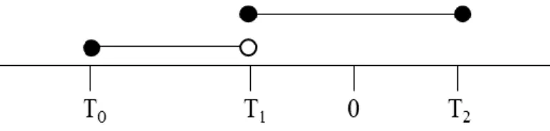
Figure 1. Representation of estimation and event window.
The estimation window is given by T0 t T1 1
13 and the event window
1 2
T t T . Let us define the length of the estimation window as(T1 1) T0 and the length of the event window as T2T1. Normally, the estimation and event window do not overlap to provide unbiased estimators for the parameters since they are not influenced by the returns surrounding the earnings announcement date. Considering day “0” as the event day, a 41-day event window is used, composed of 20 pre-announcement days and 20-post-announcement days, (-20, +20). The estimation window is defined by the interval (-371,-21), corresponding to the 250 trading days prior to the last day on the event window. It is the same method as Mackinlay (1997) uses when constructing his experimental sample. Pre-announcement interval is also considered because: i) could contribute to draw additional conclusions about stock’s behavior, ii) further investigation
12 Technically, day 0 is the day in which earnings announcement affects the market. If AMC, the next day is considered. If BMO, the same day is taken into account.
13 Hence, the interval
0 1 T . t T
9 might be attractive to understand if price movement is just noise or has some degree of inside trading and iii) does not affect current event study (instead of considering the total interval of 41 days, one just considers a 21-day interval). However, for the purpose of this paper, we focus in the post-announcement interval (from day 0 until day 20).
B. Dataset
PSI-20 Index data was gathered from 01/01/2010 until 31/12/201714. Daily closing prices
were downloaded from Bloomberg and log returns were calculated. Earnings announcement dates, information regarding after/before market announcement, earnings percentage surprise (negative, positive and neutral), companies’ market capitalization and 52-week high were also collected for the same date in all the companies of the Portuguese index.
To compute average abnormal returns and cumulative average abnormal returns one will consider all the quarterly (Q1, Q2, Q3 and Q4) announcements, from 2011-2015, with three different approaches:
1) General sample with all the earnings announcements.
2) General sample divided according to Earnings surprise: Estimated EPS > Actual Earnings (positive), Estimated EPS < Actual Earnings (negative) and no surprise (or absence of information).
3) Earnings Surprise (positive, negative and no surprise) sample is further divided according to stock’s liquidity and momentum:
14 This period selected was greater than the period of the event-study because it would be needed when incorporating 250-day estimation period and also to perform an out-of-sample back testing from 01/01/2015 until 01/01/2017.
10 a) High and low liquidity stocks. Market capitalization is used as a proxy for liquidity. PSI-20 sample is divided in a sample of stocks with mci medianmcand a sample with
i mc
mc median . 15 mc accounts for the average market cap in the last 252 trading days i
(1-year sample period) for a given stock iand medianmcfor the median market cap value
in the total sample.
b) Momentum: 52-week high is used as a proxy. Sample is divided into: i) Near to the high, ii) far from the high and iii) at the high. The groups are divided relative to the median proximity value to the high. One group accounts for all the stocks above the median value and the other for the stocks below the value. It is a similar rationale as Goh and Jeon (2017) use in their paper.
The main purpose of these three approaches is to account for different scenarios that might exacerbate or hinder the existence of abnormal returns. As new factors are incorporated in the study, results may change. In addition, daily bid-ask spreads in November 2018 are collected for every PSI-20 stocks. Opening/closing fees for stocks, borrowing costs and financing costs for CFDs are collected from SaxoBank available data.
C. Procedure
Our methodology is based on the literature of a small group of authors that studied abnormal returns around earnings season.16 In order to measure abnormal returns one has to find expected
and actual returns. Actual returns are historical values. To obtain expected return, this paper uses the market model 17. An OLS regression is performed to estimate market model’s parameters using
15 This allows for an actual 50/50 sample division, subject to minor differences due to market cap changes. 16 Brown & Warner (1980 and 1985), Mackinlay (1997), Binder (1998) and Bartholdy et al. (2005)
17 There are a wide variety of models such as the constant mean return model, multifactor model, Arbitrage pricing theory or CAPM, however the straightforwardness of the market model was a plus. Hence, this model is used throughout the paper.
11 an estimation period sample (250 trading days before the event window). In order to compute abnormal return portion in a given i stock at time t one must first compute ex-post returns.
( ) ( ) ( ) , 1 ( ) i i i i P t P t n R t n t P t n Being P ti( )the closing price of stock i at time tover a given time period of lengthn. The formula to calculate abnormal returns of security i
, ,
( ) | ( ) 2
i i t i t
AR t R E R t
The last term in the equation denotes the normal return, Ri t, | ( ) t is the ex-ante return of the stock i at period t conditioned by the information contained in the normal return model( )t . Price performance for a given security can only be perceived as abnormal relative to a particular benchmark (in this case PSI-20 index). In this case, as mentioned previously market model is used to compute expected returns, and subsequently abnormal returns. The estimated parameters, stock i and market index m are then used to compute abnormal returns. This model bears in mind only one factor of risk – equity’s beta. The model regression generates a residual in each period for every security. This residual represents the abnormal return, rather than the expected error. When the market model is used, abnormal returns are computed by the difference between actual stock returns and stock returns derived from OLS estimation.18 Market model’s expression is given by,
( ) ( )
( ) i i m 3
i i
R t
R t v tWhere R represents the actual stock i return during period t, i t, Rm t, the return of market index m during period t, the stock i model parameters and i, i v the residuals term. The i t,
conditional expected return is described as,
18 Being market index the explanatory variable.
12
, | ( ) i i m( ) 4 i t ER t R t Where 1 2 1 ( ( ) )( ( ) ) ( ( ) ) m i i m m t i i m i i m m m t R t R R t R R R R t R
.Abnormal Return is then defined as,
( ) ( ) i i m( ) 5i i
AR t R t R t
In whichAR ti( )is the abnormal stock return of stock i during period t (this is performed for every period in the event window). Then, to aggregate all the abnormal returns across every PSI-20 securities one must computeAR t , ( )
1 1 ( ) ( ) 6 n i i AR t AR t N
After computing average abnormal returns, one has to measure the cumulative average abnormal returns across stocks for the entire event window. Let us compute the average cumulative abnormal returns, which is essentially the sum of all CARs divided by the number of samples, for any interval.
2 1 1 2 1 1 ( , ) n t i( ) 7 i t CAR t t AR t N
When testing for statically significant returns one will use a parametric test that relies on the fact that returns are normally distributed.
1 2 1 2 ( , ) ~ 0, var ( , ) 8 CAR t t N CAR t t
( ) ~ 0, var ( ) 9 AR t N AR t Let us test for whether ARand CAR are statistically different from zero. The null hypothesis being tested are:
13
0a
H : There is not a significant average abnormal return at a given t during the event window due earnings announcement.
0b
H : There is not a significant cumulative average abnormal return (CAAR) at a given t
during the event window due to earnings announcements.
Hence, the cross sectional t-test for average abnormal return is defined as:
2 10 t AR AR t N Where 2 2 1 1 1 1 ( ) ( ) 1 t N N i i AR i i AR t AR t N N
.On the other hand, the t-test for the average cumulative abnormal return is given by:
, 1 2 1 2 2 ( , ) 11 t t CAR CAR CAR t t t N Where , 1 2 2 2 1 2 1 2 1 1 1 1 ( , ) ( , ) 1 t t n n i i CAR i j CAR t t CAR t t N N
forT1 t1 t2 T2.To ensure an efficient event study methodology in PSI-20 we guarantee a sample with at least 50 events to have a robust statistical significance and we also consider different samples according to stocks’ liquidity. Plus, if there is non-normality in stock returns on should use nonparametric tests instead of parametric ones.19
19 Bartholdy et al. (2005) dedicated their investigation on the efficiency of the event study methodology in less liquid stock exchanges such as the Copenhagen Stock Exchange and they concluded that event studies could be efficiently performed in small stock exchanges, but these conditions should be taken into account.
14 IV. Results and Discussion – Event-study
The results of the event study are divided in three sections. The first section presents the results of the general sample. The second section outlines the main deviations in the return’s abnormality with the introduction of a new variable: earnings surprise. The third section further divides positive, negative and no surprise stocks according to Liquidity (market cap) and momentum (52-week high). The graph (Appendix 1) exemplifies the process used in this paper. (*) means that the same factors were incorporated (to simplify process representations) in no surprise and negative surprise samples.
A. Overall Sample
This sample is composed of all 275 announcements from 2011-2015. The average cumulative abnormal return for the 21-day event is 0.19%. Average cumulative abnormal return reaches its peak at day 7 (+0.62%), pointing towards a fairly short-term drift in stock’s price as new information is assimilated by the market. Focusing on the announcement day (day 0) the average abnormal return is 0.19% (Appendix 2), with a value 1
20 of 2.05 and therefore accepting the null
hypothesis that the event has no impact on the price of a given stock. Nevertheless, days 2, 7 and 13 exhibit statistically significant abnormal returns.
B. Earnings Surprise Sample
In day 0 the three samples showed statistically significant returns (Appendix 3). In day 0, negative surprises yielded a 0.60% ARand, whereas positive surprises had the opposite behavior, with an ARof -0.38%. One possible explanation for this outcome is intra-day short term reversal,
20
1
,2correspond to the t-statistic values for the average abnormal returns and average cumulative abnormal returns, respectively.
15 meaning that strong earnings surprises (the average positive earnings surprise in the sample is 24.1%) can lead to stronger price reactions and are more likely to experience a reversal in the first trading day after the announcement (market players are likely to pursue sell-at-highs intraday strategies originating a negative average return for that day).21 The opposite rationale is also valid
for equities with negative surprises. Observing the 21-day period, CAR in positive, negative and no surprise stocks is -0.11%, -0.77% and 0.80% respectively. Negative surprises lead to a short-term portfolio adjustment (as the investor sentiment is negative) and therefore a bearish tendency is witnessed in general for every stock. Positive surprises follow a slight price correction in the following days. This is unexpected, but one possible explanation is the time that market takes to digest reported earnings and normally peak results (high surprise on earnings announced) increase investor’s risk aversion since they could mean weaker quarters in the future. If this occurs, then is very likely to observe an increase in profit taking orders, and therefore there is a price correction in the following days after a positive surprise. No surprise sample accounts for both Actual EPS = Forecasted EPS (5.15 % of the entire sample)22 and stocks with no forecasted EPS (and therefore
no reported surprise, representing 49.5% of the entire sample). No surprise category was supposed to not convey any relevant information to the market, however a positive price drift is observed. Although there are no analysts to forecast EPS, these stocks make news around earnings announcements – whether good, bad or neutral. Researchers state that these equities have high trading volume and high net buying by investors, according Attention-Grabbing Hypothesis, and therefore have a marked drift.23
21 This pattern is observed in PSI-20. For instance, stock’s price in the first hours of trading witnesses a substantial increase that tends to reverse afterwards as the amount of short positions increases.
22 This particular sample of 30 events (5.15% of the entire sample) was not considered alone due to low statistical significance. 23 According to this hypothesis, investors are net buyers of attention-grabbing stocks. Prices are therefore pushed upwards as buy orders are more than sell orders. That is, the publication issued for a given stock catches investors’ attention irrespective of their nature (positive, negative or neutral).
16 Figure 2. Plot of average cumulative returns across all events from day 0 to day 20, according to the earnings surprise. Recall that abnormal return is calculated using market model as the normal return.
C. Incorporating Momentum and Liquidity Factors
Market reaction to a stock with positive, negative or no surprise earnings could be exacerbated or hindered depending on stock’s momentum and liquidity. 52-week high is used as a proxy for momentum and three categories are explored: i) near the high (NH), ii) at the high (AH) and iii) far from the high (FH). Market capitalization is used as a proxy for liquidity and two categories are explored: i) liquid and ii) illiquid.
1. Positive Earnings Surprises
In the previous analysis, PEAD does not seem to exist for positive earnings.24 Nonetheless, this
outcome may change when exploring this sample according to stock’s momentum and liquidity. In the momentum category, within the 21-day event there is a 58.7% of abnormality in returns (Appendix 10).25 All the three sub-samples display significant abnormal returns at the
announcement date (Appendix 4), except for AH. Equities near and at the 52-week high exhibit a
24 The drift is not in the direction of an earnings surprise.
25 Number of days with significant abnormal returns as a percentage of the total days in the event window. -0.02% -0.01% -0.01% 0.00% 0.01% 0.01% 0.02% 0 1 2 3 4 5 6 7 8 9 10 11 12 13 14 15 16 17 18 19 20 CAR
17
CAR of 0.87% and 2.60% respectively. PEAD exists only for stocks at their 52-week high or near.
One possible justification is anchoring bias, since investors interpreted the impact of earnings surprises according to its proximity to the 52-week high leading them to consider that information has already been assimilated into stock’s price. Therefore, they tend to underestimate further news on the firm’s future outlook, leading to a consequent positive price drift (opposite rational for far from the high stocks). Hence, momentum explains PEAD for equities with positive earnings. On the other hand, liquidity does not clarify for PEAD, since both liquid and illiquid sub-samples (Appendix 5) yield negative CAR (-0.03% and -0.26% respectively). Although abnormal returns are significant for a substantial part of the interval (21 days), the drift is not in the same direction as the earnings surprise. Hence, there is evidence that abnormal returns around earnings announcements are not related with PEAD. Following our initial thoughts, illiquidity can exacerbate intra-day short term reversal, due to higher bid-ask spreads and the price being easily influenced by investors (high volume trading when investors want to corner the market).
Figure 3. Plot of average cumulative returns across positive surprise stocks from day 0 to day 20, according to their liquidity and momentum. -0.02% -0.01% 0.00% 0.01% 0.02% 0 1 2 3 4 5 6 7 8 9 10 11 12 13 14 15 16 17 18 19 20 CAR
18 2. Negative Earnings Surprise
PEAD seems to exist for negative surprises, specifically in liquid (Appendix 6) and far-from-high stocks (Appendix 7). FH sub-sample has a CAR of -1.09%. As previously mentioned, investors seem to interpret the impact of earnings surprises according to stock’s proximity to 52-week high. When the stock is far from the high, investors may not underestimate the impact of news and the drift moves in the same direction of the earnings surprise. AH and NH samples had positive results (3.43% and 0.90% respectively) meaning that investors relied heavily on the first piece of information given – price performance). Hence, stocks with negative earnings surprises do not witness a negative price drift when their prices are near 52-week high. One possible explanation for the outcome in liquidity sub-sample is that the return asymmetry surrounding earnings announcements is weaker for more liquid stocks because their prices reflect negative news more timely and so the drift is in the same direction as earnings surprise ( CAR of -1.64%). Conversely, asymmetry becomes stronger as liquidity risk increases ( CAR of 0.19%).
Figure 4. Plot of average cumulative returns across negative surprise stocks from day 0 to day 20, according to their liquidity and momentum. -0.03% -0.02% -0.01% 0.00% 0.01% 0.02% 0.03% 0.04% 0 1 2 3 4 5 6 7 8 9 10 11 12 13 14 15 16 17 18 19 20 CAR
19 3. No Surprise
At the announcement date, if a given stock is AH, NH or FH (Appendix 8) it shows a CAR of -3.27%, 0.51% and 1.07% respectively. Stocks far from the high experience a more positive drift since investors tend to have lack of hard reporting data, and therefore exists a higher upside potential for speculation when compared with stocks closer to their 1-year historical maximum. The opposite rationale is also valid, and therefore NH sub-sample experienced the higher price correction. All categories show significant ARat the announcement date, except for NH category. Liquid equities (evidence of ARin day 0) show a higher CAR (Appendix 9) than illiquid stocks (1.01% vs. 0.38%). Companies with no surprise are more illiquid than companies with positive/negative surprises, possibly because of a higher information asymmetry or uncertainty among released news, therefore makes sense that the price drift in no surprise category is mainly influenced by illiquid stocks.
Figure 5. Plot of average cumulative returns across no surprise stocks from day 0 to day 20, according to their liquidity and momentum. -0.04% -0.02% 0.00% 0.02% 1 2 3 4 5 6 7 8 9 10 11 12 13 14 15 16 17 18 19 20 21 CAR
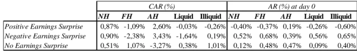
20 Overall, investors’ trading relies more on stock’s momentum rather than earnings surprise (whether positive or negative). On the other, if there is absence of hard data release (no earnings surprise) speculative investment explains the drift (rather than anchoring bias). The table below summarizes the average abnormal return (at the announcement day) and average cumulative abnormal return during the 21-day event window:
Table 1 – Average AR (at day 0) and CAR in the event window, according to stock’s liquidity and momentum.
V. Results and Discussion – Investment Strategy
After using an event-study methodology to test the significance of ARand CAR , this paper intends to implement a feasible investment strategy (accounting for transaction costs) that mimics major findings in the previous event study. Chordia (2009) showed that transaction costs inhibit the exploitation of PEAD. The period of the out-of-sample back testing is performed from 01-01-2015 until 01-01-2017. On this paper we develop 8 trading strategies with a 20 days holding period. This paper seeks to improve trading strategies by incorporating new variables, as explained before. These strategies are Equity-Long Only and Equity Long-Short. Generally, for long positions a
return of ln t n X k X
is generated, where for short positions a return of ln
t n X k i s X is
obtained. Xt is the opening price of the stock at day 1 (one day after market reaction to the announcement) and Xn represents the last day of the holding period (in this case, day 20). k
represents the transactions costs including bid-ask spread and opening/closing fee, i the borrowing costs and s the financing costs.
NH FH AH Liquid Illiquid NH FH AH Liquid Illiquid
Positive Earnings Surprise 0,87% -1,09% 2,60% -0,03% -0,26% -0,40% -0,37% 0,19% -0,26% -0,60%
Negative Earnings Surprise 0,90% -2,38% 3,43% -1,64% 0,19% 0,52% 0,68% 0,39% 0,56% 0,65%
No Earnings Surprise 0,51% 1,07% -3,27% 0,38% 1,01% 0,12% 0,48% 0,47% 0,09% 0,40%
21 A. Transaction costs and Short-selling
In the Portuguese stock market, liquidity is an important issue, and therefore transaction costs for long (Appendix 11) and short positions (Appendix 12) should be precisely incorporated. Transactions costs included are:
a) Bid-ask spread: Average bid-ask spread specific for each company in the Portuguese stock index is computed (illiquidity tends to increase bid-ask spread). Historical data from daily closing prices, in the last month (November 2018), was collected for all companies in PSI-20.
b) Initial fee: fee incurred when opening/closing positions. A total value (for opening and closing a long/short position in a given stock) of 10 bps is used (average cost applied by brokers in Portugal).
c) Borrowing and Financing costs: for the average investor short selling equities in Portuguese market could be performed using CFDs (10 bps is also used as opening and closing fee). First, the financing costs associated with this derivative, with a holding period higher than
one day, is an interest equivalent toLIBID Fixed Spread Holding Period in days 360
.
26
The fixed spread is 3% and LIBID is -0.456%.27 For short positions, there exist also
borrowing costs that depend on the liquidity of the underlying stocks, hence borrowing costs are liquidity-specific and vary across stocks. Note that is not possible to short sell all stocks available in PSI-20 due to high liquidity risk (their short sell status in constantly
26 When holding a short position in CFDs, the investor receives a credit calculated based on the relevant inter-bank bid rate depending on the currency of the underlying asset deducted from a fixed mark-up (spread). If the calculated financing costs in a short position are negative, the financing credit is, in fact, a financing charge. Values provided by SaxoBank.
27 LIBID rate is not publicly available, therefore we used LIBOR rate minus 1/8 of 1% (by convention) as a proxy. 11 December 2018 Euro LIBOR overnight rate was used and collected from Intercontinental Exchange (ICE).
22 changing due to market and liquidity conditions). Nonetheless, this paper assumes theoretically that it is possible to enter in a short position for every single stock.28
d) Spread CFD/Equity: the difference between tradable bid and ask prices between CFDs and its underlying, equity. One will consider 10 bps as an average spread in PSI-20 stocks.29
B. Rationale and Results of Investment Strategies
These strategies are based on the patterns observed in section Results and Discussion. Overall Strategy (Strategy 1) takes advantage of PEAD (positive drift) in PSI-20 and therefore a long-only portfolio is designed. Earnings Surprise Strategy (Strategy 2) also considers earnings surprise (positive, negative or no surprise) and goes long on companies that have no surprise on their EPS surprise (explained by attention-grabbing hypothesis) and short companies that positive (due to intra-day short term reversal) and negative surprises (due to negative price drift). Positive earnings with momentum strategy (Strategy 3) is designed with a long position in AH/NH stock’s with positive earnings and short on FH equities. Anchoring bias, as mentioned before, is the rationale behind the trading strategy. Positive surprises with Liquidity strategy (Strategy 4) is an equity-short only strategy, with short positions in bot liquid and illiquid equities with positive surprises (since it enhances intra-day short term reversal). Negative Surprises with momentum strategy (Strategy
5) relies on the investor’s misinterpretation of stock’s nearness to 52-week high (mentioned
earlier), with long positions in AH and NH, and short positions in FH stocks. Negative surprises with liquidity strategy (Strategy 6) goes long on illiquid stocks (return asymmetry surrounding earnings announcements increases with illiquidity) and short on liquid firms (negative price drift). No surprises with momentum strategy (Strategy 7) is a Long-short equity strategy, going short AH
28 In this case, borrowing cost assumed are the average borrowing cost in the Portuguese stock market for the companies that is possible to short sell plus 1% called a liquidity premium.
23 firms and long on FH and NH (no hard data to support the decision and therefore upside potential for speculation is higher for stocks far from 52-week high). No surprises with liquidity strategy (strategy 8) is a long-only equity strategy with long positions on liquid and illiquid firms with no surprises (attention-grabbing hypothesis is enhanced as illiquidity increases). The following table presents the results for the 8 strategies implemented:
Table 2 – Comparison between trading strategies.
The following graph shows the pattern of cumulative returns for the 8 strategies designed:
Figure 6. Cumulative return of the Trading strategies (1-8) implemented, during the 20-day holding period.
To have a successful strategy, the trading strategy should have an optimal accuracy and risk to reward ratio. As it can be concluded from the analysis of the average cumulative return (net return, including transaction costs) during the 20-day holding period just one strategy presents
Info Sharpe Annualized Retun Volatility % Positive days % negative days Max Drawdown Skewness Kurtosis Accuracy Average TC/day
Strategy 1 0,49 1,24% 2,54% 55,00% 45,00% -0,87% -0,38 0,69 57,55% 0,02% Strategy 2 1,13 6,03% 5,36% 61,67% 38,33% -1,28% -0,32 -0,13 59,71% 0,05% Strategy 3 0,20 2,32% 11,50% 51,67% 48,33% -1,25% 0,88 1,77 56,76% 0,05% Strategy 4 1,47 37,47% 25,48% 62,50% 37,50% -3,47% -0,58 0,62 51,43% 0,06% Strategy 5 -0,63 -10,52% 16,82% 55,00% 45,00% -4,37% -0,44 3,28 41,67% 0,04% Strategy 6 0,01 0,32% 35,69% 52,50% 47,50% -2,94% 0,92 2,74 63,64% 0,04% Strategy 7 1,78 23,57% 13,21% 58,33% 41,67% -2,39% -0,68 3,07 65,12% 0,04% Strategy 8 1,61 26,35% 16,33% 65,00% 35,00% -1,86% -0,18 0,62 64,63% 0,02% -0.03% -0.02% -0.01% 0.00% 0.01% 0.02% 0.03% 0.04% 1 2 3 4 5 6 7 8 9 10 11 12 13 14 15 16 17 18 19 20 C um ul at iv e Ret ur n
Strategy 3 Strategy 2 Strategy 5 Strategy 1
24 negative return. Therefore, strategy 5 is not worthy to engage (IS < 0). Moreover, the presence of high drawdowns (relative to the 20-day period) in strategies 4 and 5 hinders the possible implementation of such models. It seems that strategy 7 has the best risk-return reward, being translated into a higher Sharpe ratio. With strategies 7 and 8 we achieve a better accuracy (65.12% and 64.63%) and maximum Sharpe ratio of 1.78 and 1.61, respectively. Strategy 8 experiences more stable cumulative returns and lower drawdowns (Table 2). In fact, we conclude that strategy
8 results in an optimized and more consistent strategy that outperforms the others. Additionally,
the average cumulative return considering all the 8 strategies is 1.62%, and the average transaction costs for the 20-day holding period performs a total of 78bp. This accounts for 48.5% of the average cumulative returns. Just as an example, strategy 1 yields an Info Sharpe of 0.49 (when including transaction costs) versus 2.49 without. Therefore, engaging in short-term trading strategies like these ones substantially hinder profits. Illiquidity (larger bid-ask spreads) and short-selling increase significantly transaction costs. 30
The main findings of this paper are consistent with previous results on the subject. Similarly to Alves and Santos (2005), who presents a relationship between financial information announced quarterly and investor’s decisions, our event-study on PSI-20 showed the existence of abnormal returns in the days 2, 7 and 13. Moreover, in agreement with Chordia (2009) we conclude that transaction costs do reduce PEAD, however do not inhibit it. When incorporating new factors like momentum, we must agree with Goh and Jeon (2017) that investors interpret impact of earnings news based on stock’s nearness to 52-week high, as the percentage of abnormality in the event window increases significantly with momentum. Additionally, our findings are in line with Schmitz (2007) since we find a larger drift for negative than positive stock’s surprises. Nonetheless,
25 most research papers disregard the potential of firms that do not have an EPS surprise (in line with forecasted or no analysts to forecast it), mainly with stocks trading in less liquid markets. Quite the opposite, we conclude that despite its increased volatility, trading stocks in PSI-20 which do not convey hard reporting data to the market, based on liquidity and momentum factors can yield an optimal financial performance in terms of Sharpe ratio and success rate (accuracy). In fact our findings are different from Forbes and Giannopoulos (2015) as we conclude that an increase in information uncertainty increased the strength of observed post-announcement earnings drift.
VI. Conclusion
In this paper, we study if there are abnormal returns in PSI-20 around earnings announcements. The present study focus on momentum and liquidity as factors that might affect post-announcement drift according to the surprise in each announcement, for every firm. First, we found that abnormal returns do exist in PSI-20. In fact, this market inefficiency is exacerbated when we compute abnormal returns for positive, negative and no surprises according to momentum and liquidity. Second, the out-of-sample results obtained in the investment strategies are robust except for negative earnings surprise with momentum (and therefore not generating a profitable trading strategy). Indeed, we demonstrated that that 50% of the trading strategies implemented yield an info Sharpe greater than one. Third, we concluded that transaction costs affect the profitability of trading strategies, and showed that the average cumulative returns are significantly lower when we include transaction costs. Overall, despite the presented drawbacks and assumptions, we conclude that there is the potential to take advantage of PEAD in PSI-20 to make feasible and efficient investment strategies. As for future researches, the event-study should be complemented with a pre-announcement analysis to study the extent at which PEAD is hindered by market inefficiencies prior to the announcement.
26 VII. References
[1] Alves, Carlos F., and F. Teixeira dos Santos. 2005. “The Informativeness of Quarterly Financial Reporting: The Portuguese Case.” CEMPRE – Centro de estudos Macroeconómicos e
Previsão, 177.
[2] Ball, Ray and Lakshmanan Shivakumar. 2008. “How much new information is there in earnings?” Journal of Accounting Research, 46 (5): 975-1016.
[3] Ball, Ray, and Philip Brown. 1968. “An Empirical Evaluation of Accounting Numbers.”
Journal of Accounting Research, 6: 159-178.
[4] Bartholdy, Jan, Dennis Olson, and Paula Peare. 2005. “Conducting event studies on a small stock exchange.” Arhus School of Business – Department of Finance.
[5] Beaver, William. 1968. “The information content of annual earnings announcements.”
Journal of Accounting Research, 6: 67-92.
[6] Bernard, Victor and Jacob K. Thomas. 1989. “Post-Earnings-Announcement Drift: Delayed Price Response or Risk Premium?” Journal of Accounting Research, 27: 1-36.
[7] Binder, John. 1998. “The event study methodology since 1969.” Review of Quantitative
Finance and Accounting, 11: 111-137.
[8] Brandt, Michael W., Runnet Kishore, Pedro Santa-Clara, and Mohan Venkatachalam. 2008. “Earnings announcements are full of surprises”.
[9] Brown, Stephen J., and Jerold B. Warner. 1980. “Measuring security price performance.”
27 [10] Brown, Stephen J., and Jerold B. Warner. 1985. “Using daily stock returns: the case of event studies.” Journal of Financial Economics, 14: 3-31.
[11] Chen, Carl R., James Wuh Lin, and David A. Sauer. 1997. “Earnings announcements, quality and quantity of information, and stock price changes.” The Journal of Financial Research, 20 (4): 483-502.
[12] Chen, XiaoHua, Edna Solomon, and Thanos Verousis. 2016. "Asymmetric Post-Announcement Drift to Good and Bad News: Evidence from Voluntary Trading Disclosures in the Chinese Stock Market." International Journal of the Economics of Business, 23 (2): 183-198. [13] Chordia, Tarun, Amit Goyal, Ronnie Sadka, and Lakshmanan Shivakumar, 2009. “Liquidity and the Post-Earnings Announcement Drift.” Financial Analysts Journal, 65 (4).
[14] Chudek, Mark, Cameron Truong, and Madhu Veeraraghavan. 2011. "Is trading on earnings surprises a profitable strategy? Canadian evidence." Journal of International Financial Markets,
Institutions and Money, 21 (5): 832-850.
[15] Fama, Eugene F. 1970. “Efficient Capital Markets: A review of Theory and Empirical Work.” The Journal of Finance, 25 (2): 383-417.
[16] Fama, Eugene F. 1998. “Market efficiency, long-term returns and behavioral finance.”
Journal of Financial Economics, 49 (2): 283-306.
[17] Forbes, William, and George Giannopoulos. 2015. “Post-Earnings Announcement Drift in Greece.” Review of Pacific Basin Financial Markets and Policies, 18 (3).
[18] Forner, Carlos, Sonia Sanabria, and Joaquín Marhuenda. 2009. “Post-Earnings Announcement Drift: Spanish Evidence”, Spanish Economic review, 11 (3):207-241.
28 [19] Foster, Chris Olsen and Terry Shevlin. 1984. “Earnings release, anomalies, and the behavior of security returns.” The Accounting Review, 59 (4)
[20] Goh, Jihoon, and Byoung Hyun Jeon. 2017. “Post-earnings-announcement-drift and 52-week high: Evidence from Korea.” Pacific-Basin Finance Journal, 44: 150-159.
[21] Jones, Charles P., and Robert H. Litzenberger. 1970. “Quarterly Earnings reports and intermediate stock price trends.” The Journal of Finance, 25 (1): 143-148.
[22] Joy, Maurice O., Robert H. Litzevberger, R. and Richard W. McEnally. 1977. “The Adjustment of Stock Prices to Announcements of Unanticipated Changes in Quarterly Earnings.”
Journal of Accounting Research, 15 (2): 207-225.
[23] Liu, Weimin, Norman C. Strong, and Xinzhong. Xu. 2001. “Post-earnings-announcement drift in the UK.”
[24] Lourenço, António, and Maria Coelho. 2008. “Conteúdo informativo do resultado anual na Euronext Lisbon.”, Proelium – revista da Academia Militar, 10.
Mackinlay, Craig. 1997. “Event studies in Economics and Finance.” Journal of Economic
Literature, 35: 13-39.
[25] May, Robert G., 1971. “The influence of Quarterly Earnings announcements on investor decisions as reflected in common stock price changes.” Journal of Accounting Research, 9: 119-163.
[26] N.G., Jeffrey, Tjomme O. Rusticus, and Rodrigo S. Verdi. 2008. "Implications of Transaction Costs for the Post-Earnings Announcement Drift." Journal of Accounting Research, 46 (3): 661-696.
29 [27] Pinto, Inês. 2003. “O impacto da divulgação dos factos relevantes no mercado de capitais português”, Instituto Superior de Ciências do Trabalho e da Empresa, Tese de Mestrado.
[28] Romacho, João Carlos, and Vânia Gaspar Cidrais. 2007. “A eficiência do mercado de capitais português e o anúncio dos resultados contabilísticos.” Tékhne – Polytechnical Studies
Review, 4 (7).
[29] Schmitz, Philipp. 2007. “Market and individual investors’ reactions to corporate news in the media.”
[30] Truong, Cameron. 2010. “Post earnings announcement drift and the roles of drift-enhanced factors in New Zealand.” Pacific-Basin Finance Journal, 18 (2):139-157.
[31] Truong, Cameron. 2011. “Post-earnings announcement abnormal return in the Chinese equity market.” Journal of International FinancialMarkets, Institutions and Money, 21 (5): 637- 661.
[32] Wael, Louhichi. 2004. “Market reaction to annual earnings announcements: the case of the Euronext Paris.”
[33] Wilton, Pedro. 2002. “Impacto da Divulgação de Resultados na Negociação em Mercado de Bolsa.” Cadernos do Mercado de Valores Mobiliários - CMVM, 15.
[34] Zhang, Qi, Charlie X. Cai, and Kevin Keasey. 2013. "The profitability, costs and systematic risk of the post-earnings-announcement-drift trading strategy." Review of Quantitative Finance and
Accounting, 43 (3): 605-625.
[35] Cervellati, Enrico, Riccardo Ferretti and Pierpaolo Pattitoni. 2014. “Market Reaction to second-hand news: inside the attention grabbing hypothesis.” Applied Economics, 46 (10): 1108-1121.
30 VIII. Appendix
Appendix 1 - Example of the process used in the paper, when incorporating new variables to account for abnormal returns.
Appendix 2 – Average abnormal and cumulative abnormal returns in the overall sample from 2011-2015.
All earnings announcements AR All earnings announcements CAR
Ove rall Ove rall
0 0,19% 0,19% 1 -0,09% 0,09% 2 0,23% 0,32% 3 0,02% 0,34% 4 0,08% 0,42% 5 0,05% 0,46% 6 -0,04% 0,42% 7 0,20% 0,62% 8 -0,06% 0,56% 9 -0,10% 0,45% 10 -0,12% 0,34% 11 0,02% 0,35% 12 -0,13% 0,22% 13 0,18% 0,40% 14 0,00% 0,40% 15 -0,01% 0,39% 16 -0,02% 0,37% 17 -0,02% 0,34% 18 -0,04% 0,31% 19 -0,14% 0,17% 20 0,02% 0,19%
31
Appendix 3 – Average abnormal and cumulative abnormal returns according to different earnings surprises, from 2011-2015.
Appendix 4 – Average abnormal and cumulative abnormal returns for positive earnings surprises according to stock’s
momentum from 2011-2015.
No Surprise Negative Surprise Positive Surprise No Surprise Negative Surprise Positive Surprise
0 0,31% 0,60% -0,38% 0,31% 0,60% -0,38% 1 -0,14% -0,27% 0,15% 0,16% 0,33% -0,24% 2 0,17% 0,16% 0,39% 0,33% 0,50% 0,16% 3 -0,05% 0,26% -0,07% 0,29% 0,75% 0,09% 4 0,18% -0,12% 0,07% 0,46% 0,64% 0,15% 5 0,32% -0,18% -0,27% 0,78% 0,46% -0,12% 6 0,00% -0,12% -0,06% 0,78% 0,33% -0,18% 7 0,28% 0,05% 0,15% 1,07% 0,39% -0,03% 8 0,23% -0,44% -0,27% 1,29% -0,06% -0,29% 9 -0,04% -0,18% -0,17% 1,26% -0,23% -0,46% 10 -0,18% -0,30% 0,15% 1,08% -0,53% -0,31% 11 0,05% -0,13% 0,09% 1,12% -0,66% -0,22% 12 -0,22% -0,11% 0,02% 0,91% -0,77% -0,20% 13 0,37% 0,10% -0,12% 1,28% -0,67% -0,33% 14 -0,08% 0,03% 0,12% 1,21% -0,65% -0,21% 15 -0,11% 0,00% 0,16% 1,10% -0,65% -0,05% 16 0,18% -0,16% -0,28% 1,28% -0,81% -0,33% 17 -0,07% 0,13% -0,06% 1,20% -0,68% -0,39% 18 -0,26% 0,47% -0,04% 0,94% -0,21% -0,44% 19 -0,22% -0,31% 0,17% 0,72% -0,52% -0,27% 20 0,08% -0,25% 0,16% 0,80% -0,77% -0,11%
Earnings Surprise AR Earnings Surprise CAR
Near High Far High At High Near High Far High At High
0 -0,40% -0,37% 0,19% -0,40% -0,37% 0,19% 1 0,30% -0,01% 0,55% -0,10% -0,38% 0,74% 2 0,09% 0,69% -0,09% 0,00% 0,31% 0,65% 3 0,09% -0,23% 0,89% 0,09% 0,08% 1,54% 4 0,32% -0,19% 0,58% 0,41% -0,10% 2,12% 5 -0,23% -0,31% -0,85% 0,18% -0,41% 1,27% 6 -0,31% 0,20% -0,46% -0,14% -0,21% 0,81% 7 0,13% 0,17% 0,36% -0,01% -0,04% 1,17% 8 -0,27% -0,27% 0,03% -0,27% -0,31% 1,20% 9 -0,27% -0,06% -0,11% -0,54% -0,37% 1,09% 10 0,40% -0,11% -0,05% -0,14% -0,48% 1,04% 11 0,08% 0,10% -0,24% -0,06% -0,38% 0,79% 12 0,40% -0,37% 0,68% 0,34% -0,75% 1,47% 13 -0,27% 0,03% -0,56% 0,07% -0,72% 0,91% 14 0,12% 0,12% 0,28% 0,19% -0,60% 1,20% 15 0,26% 0,06% 0,64% 0,45% -0,54% 1,83% 16 -0,04% -0,53% 0,22% 0,41% -1,07% 2,05% 17 0,23% -0,36% 0,07% 0,64% -1,43% 2,12% 18 -0,05% -0,04% -0,36% 0,59% -1,47% 1,76% 19 -0,01% 0,34% 0,20% 0,58% -1,13% 1,95% 20 0,29% 0,03% 0,64% 0,87% -1,09% 2,60%
32
Appendix 5 – Average abnormal and cumulative abnormal returns for positive earnings surprises according to stock’s liquidity
from 2011-2015.
Appendix 6 – Average abnormal and cumulative abnormal returns for negative earnings surprises according to stock’s liquidity
from 2011-2015.
Liquid Illiquid Liquid Illiquid
0 -0,26% -0,60% -0,26% -0,60% 1 0,10% 0,24% -0,17% -0,37% 2 0,52% 0,16% 0,35% -0,20% 3 0,04% -0,27% 0,39% -0,48% 4 -0,04% 0,26% 0,35% -0,22% 5 -0,05% -0,68% 0,30% -0,90% 6 0,05% -0,26% 0,36% -1,16% 7 0,19% 0,07% 0,55% -1,09% 8 -0,26% -0,28% 0,29% -1,37% 9 -0,30% 0,09% -0,01% -1,28% 10 0,01% 0,40% 0,00% -0,88% 11 -0,03% 0,31% -0,03% -0,57% 12 0,15% -0,22% 0,12% -0,79% 13 -0,05% -0,26% 0,07% -1,05% 14 0,05% 0,24% 0,12% -0,81% 15 -0,20% 0,82% -0,08% 0,01% 16 -0,14% -0,55% -0,22% -0,54% 17 -0,02% -0,13% -0,24% -0,68% 18 -0,30% 0,44% -0,55% -0,24% 19 0,24% 0,03% -0,31% -0,20% 20 0,28% -0,06% -0,03% -0,26%
Positive earnings surprise and Liquidity AR Positive earnings surprise and Liquidity CAR
Liquid Illiquid Liquid Illiquid
0 0,56% 0,65% 0,56% 0,65% 1 -0,54% 0,03% 0,02% 0,68% 2 0,23% 0,08% 0,25% 0,76% 3 0,30% 0,21% 0,55% 0,97% 4 -0,05% -0,19% 0,50% 0,79% 5 0,11% -0,50% 0,61% 0,29% 6 -0,25% 0,02% 0,35% 0,31% 7 -0,55% 0,71% -0,19% 1,02% 8 -0,35% -0,54% -0,55% 0,48% 9 -0,31% -0,03% -0,86% 0,46% 10 -0,28% -0,31% -1,14% 0,15% 11 -0,19% -0,07% -1,33% 0,08% 12 -0,12% -0,11% -1,45% -0,03% 13 -0,05% 0,27% -1,50% 0,23% 14 -0,12% 0,18% -1,61% 0,42% 15 -0,16% 0,17% -1,78% 0,59% 16 -0,13% -0,19% -1,91% 0,40% 17 0,41% -0,17% -1,51% 0,23% 18 0,36% 0,60% -1,15% 0,82% 19 -0,31% -0,30% -1,46% 0,53% 20 -0,18% -0,33% -1,64% 0,19%
33
Appendix 7 – Average abnormal and cumulative abnormal returns for negative earnings surprises according to stock’s
momentum from 2011-2015.
Appendix 8 – Average abnormal and cumulative abnormal returns for no earnings surprises according to stock’s momentum
from 2011-2015.
Near High Far High At High Near High Far High At High
0 0,52% 0,68% 0,39% 0,52% 0,68% 0,39% 1 -0,58% 0,04% 0,13% -0,06% 0,72% 0,52% 2 0,11% 0,22% 0,74% 0,05% 0,93% 1,25% 3 0,30% 0,22% 0,50% 0,35% 1,15% 1,76% 4 0,03% -0,26% 0,32% 0,38% 0,89% 2,08% 5 0,22% -0,57% 0,54% 0,60% 0,32% 2,62% 6 0,01% -0,25% -0,36% 0,61% 0,07% 2,26% 7 0,04% 0,06% -0,09% 0,65% 0,13% 2,17% 8 0,29% -1,16% 0,42% 0,95% -1,03% 2,59% 9 -0,10% -0,25% 0,28% 0,84% -1,27% 2,87% 10 -0,51% -0,09% -0,35% 0,34% -1,36% 2,52% 11 0,19% -0,44% -0,41% 0,52% -1,81% 2,10% 12 0,32% -0,53% 0,78% 0,84% -2,34% 2,89% 13 -0,14% 0,34% 0,20% 0,70% -2,00% 3,09% 14 0,09% -0,04% 0,23% 0,79% -2,04% 3,32% 15 0,24% -0,24% -0,85% 1,03% -2,28% 2,47% 16 0,11% -0,42% -0,59% 1,14% -2,70% 1,88% 17 -0,04% 0,29% 0,54% 1,10% -2,41% 2,42% 18 0,12% 0,81% 0,16% 1,22% -1,60% 2,58% 19 -0,25% -0,36% 0,12% 0,97% -1,96% 2,69% 20 -0,07% -0,43% 0,73% 0,90% -2,38% 3,43%
Negative earnings surprise and Momentum AR Negative earnings surprise and Momentum CAR
Near High Far High At High Near High Far High At High
0 0,12% 0,48% 0,47% 0,12% 0,48% 0,47% 1 -0,36% 0,06% -0,78% -0,24% 0,54% -0,31% 2 0,14% 0,20% 0,27% -0,10% 0,74% -0,04% 3 -0,08% -0,02% -1,44% -0,18% 0,72% -1,49% 4 0,37% 0,00% -0,49% 0,19% 0,72% -1,98% 5 0,01% 0,61% -1,56% 0,20% 1,33% -3,54% 6 0,12% -0,11% 0,43% 0,33% 1,21% -3,12% 7 0,02% 0,53% 0,17% 0,35% 1,75% -2,94% 8 0,39% 0,07% 1,67% 0,74% 1,82% -1,28% 9 -0,08% 0,01% 0,02% 0,66% 1,82% -1,25% 10 0,25% -0,58% 0,68% 0,90% 1,24% -0,57% 11 0,18% -0,08% -0,20% 1,08% 1,16% -0,77% 12 -0,46% 0,01% -1,81% 0,62% 1,17% -2,58% 13 0,26% 0,48% 0,23% 0,89% 1,65% -2,35% 14 -0,05% -0,10% -0,17% 0,84% 1,55% -2,51% 15 0,07% -0,28% -0,29% 0,91% 1,28% -2,80% 16 0,04% 0,31% 0,16% 0,95% 1,59% -2,64% 17 -0,07% -0,08% -1,09% 0,88% 1,50% -3,73% 18 -0,07% -0,44% 0,30% 0,81% 1,06% -3,43% 19 -0,17% -0,27% -0,03% 0,64% 0,79% -3,46% 20 -0,14% 0,28% 0,19% 0,51% 1,07% -3,27%
34
Appendix 9 – Average abnormal and cumulative abnormal returns for no earnings surprises according to stock’s liquidity from
2011-2015.
Appendix 10 – Percentage of average AR and CAR in the event window
Appendix 11 – Average transaction costs (TTC day) in Long positions.
Appendix 12 – Average transaction costs (TTC day) in Short positions.
Liquid Illiquid Liquid Illiquid
0 0,09% 0,40% 0,09% 0,40% 1 0,15% -0,27% 0,24% 0,13% 2 -0,20% 0,33% 0,04% 0,46% 3 0,10% -0,10% 0,14% 0,35% 4 0,22% 0,16% 0,36% 0,51% 5 0,38% 0,30% 0,74% 0,81% 6 -0,12% 0,05% 0,62% 0,86% 7 0,05% 0,39% 0,67% 1,25% 8 0,29% 0,20% 0,96% 1,45% 9 -0,08% -0,03% 0,88% 1,42% 10 -0,12% -0,21% 0,76% 1,21% 11 -0,07% 0,09% 0,69% 1,30% 12 -0,07% -0,30% 0,62% 1,00% 13 0,29% 0,42% 0,92% 1,42% 14 0,14% -0,17% 1,05% 1,25% 15 -0,11% -0,11% 0,95% 1,14% 16 -0,12% 0,32% 0,83% 1,46% 17 -0,33% 0,10% 0,50% 1,55% 18 0,23% -0,50% 0,73% 1,06% 19 -0,08% -0,29% 0,65% 0,77% 20 -0,26% 0,24% 0,38% 1,01%
No earnings surprise and Liquidity AR No earnings surprise and Liquidity CAR
Samples % of AR % of CAR
Overall 14,29% 14,29%
Ernings Surprise 46,03% 47,62%
Positive Surprise + Momentum 66,67% 58,73% Negative Surprise + Momentum 73,02% 90,48% No Surprise + Momentum 47,62% 80,95% Positive Surprise + Liquidity 61,90% 45,24% Negative Surprise + Liquidity 76,19% 61,90% No Surprise + Liquidity 52,38% 64,29% Trading Days Long Positions 20 Initial Fee 0,10% 0,01% Bid/Ask Spread 0,38% 0,02% TTC day 0,48% 0,02% Trading Days Short Positions 20 Initial Fee 0,10% 0,01% Bid/ask Spread 0,38% 0,02% CFD/Equity Spread 0,10% 0,01% Financiang Costs -0,03% Borrowing Costs 0,003% TTC day 0,06%