S
tock
returnS
and
volatility
:
the
B
razilian
caSe
*
Benjamin M. tabak§
Solange M. Guerra¤
reSuMo
Este artigo examina a relação entre retornos de ações e volatilidade no período de junho de 1990 a abril de 2002. Estudamos a relação entre retornos de ações e volatilidade no nível da firma para uma amostra de 25 séries de ações brasileiras. Usando o método de regressões aparentemente não relacionadas (SUR) a evidência empírica sugere que retornos contemporâneos e volatilidades estão positivamente e significativamente rela-cionados enquanto existe relação negativa entre mudanças de volatilidade e retornos de ações. Finalmente, o efeito de assimetria na volatilidade é consistente com as ações brasileiras como pode ser percebido dos re-sultados da estimação AR(1)-EGARCH(1,1).
Palavras-chave: retornos de ações, volatilidade, regressões aparentemente não relacionadas, EGARCH.
aBStract
This paper examines the relationship between stock returns and volatility over the period of June 1990 to April 2002. We study firm-level relationship between stock returns and volatility for a sample of 25 time series of Brazilian stocks. Using Seemingly Unrelated Regressions (SUR) empirical evidence suggests that contemporaneous returns and volatilities are significantly and positively correlated while there is a negative relationship between changes in volatility and stock returns. Finally, the asymmetric volatility effect seems to hold for Brazilian stocks as shown by the results from an AR(1)-EGARCH(1,1) estimation.
key words: stock returns, volatility, Seemingly Unrelated Regressions, EGARCH.
* The authors thank two anonymous reviewers, which have helped improve the paper. The opinions expressed in the paper are those of the authors and do not reflect those of the Banco Central do Brasil. Benjamin M. Tabak gratefully acknowledges financial support from CNPQ Foundation.
§ Banco Central do Brasil, Research Department. SBS – Quadra 3 – Bloco B – Ed. Sede. CEP 70074-900 – Brasília – DF. E-mail: benjamin@ucb.br.
1 i
ntroductionThe seminal work of Markowitz (1952), which developed the basic portfolio theory, derived a linear relationship between risk and return, which in turn proved to be useful for portfolio and asset management, and also for asset and derivatives pricing. Since this seminal work much resear-ch has been done investigating the relationship between stock returns and volatility for developed markets. Uncovering the relationship between risk and return provides a better understanding of price dynamics and can serve as a guide for building new asset pricing models.
Furthermore, Black (1976) and Christie (1982), two authors that have also studied the risk-return relationship, found that stock prices declines for individual firms raises financial leverage, which resulted in an increase in equity’s volatility. A negative relationship between changes in vo-latility and stock returns was found.
Following a similar line of research, Cheung and Ng (1992) using EGARCH models also found evidence of a negative relationship between the log of the one-day-ahead conditional volati-lity and stock returns.
This effect is commonly known in the literature as the leverage effect. Black (1976) argued that a fall in a firm’s stock value relative to the market value of its debt unleashes a rise in its debt-equity ratio and in the stock volatility. From this set of papers the foremost message was that an important channel for the risk-return relationship was financial leverage (debt-to-equity ratio) for individual firms.
When examining the intertemporal relationship between volatility and expected returns for the U.S., French, Schwert and Stambaugh (1987) found evidence that the expected market risk premium is positively related to the volatility of stock returns. Cheung and Ng (1992) analyze the relation between stock price dynamics and firm size. Evidence found shows that conditional future volatility of equity returns is negatively related to the level of stock price. The results also reveal that this effect is stronger for small firms with higher financial leverage.
In the same line, Theodossiou and Lee (1995) inspect the intertemporal relationship betwe-en risk and expected return for tbetwe-en industrialized countries. The authors use a GARCH in mean model and test for the conditional variance and expected market return relationship. They found no significant relationship between conditional volatility and expected return for any of these countries. Following this idea, Mougoué and Whyte (1996) study the connection between stock returns and volatility for the German and French equity markets. They have found that the impact of volatility on stock returns is insignificant.
Moreover, De Santis and Imrohoroglu (1997) study the dynamics of expected returns and volatility for emerging markets. The results evince that the level of volatility in emerging markets is considerably higher than that of more mature markets. They also scrutinize the issue of whether liberalization would increase/decrease volatility. They found evidence suggesting that country-spe-cific risk does not play any role in explaining conditional expected returns.
This paper tests whether there is a contemporaneous relation between stock returns and cur-rent and future volatility for Brazilian stocks, employing Seemingly Unrelated Regressions. The data covers the period of June 1990 to April 2002. A robustness test has been done analyzing two sub-periods. The first sub-period covers June 1990 to July 1994 while the second August 1994 to April 2002, to account for changes in the stock market due to the Real stabilization plan, which has been successful in reducing inflation in Brazil. Empirical evidence suggests that as in the U.S. case studied by Duffee (1995), Brazilian stocks have a positive relationship between stock returns and contemporaneous volatility. Furthermore, using nonparametric techniques we test for firm size, market capitalization and debt/equity ratios as potential explanatory variables for the results found.
Brazil is one of the most important countries in Latin America and accounts for more than 40% of the region’s market capitalization. Furthermore, it has a high volatility environment and has had a structural change in the mid-nineties, which makes it an interesting case to study whe-ther the leverage effect would hold in this environment.
To the best of our knowledge this is the first paper that addresses the relationship between volatility and stock returns for the Brazilian stock market. This paper focuses on this relationship using two methodologies. One using single regressions methods for the most liquid stocks and Nelson’s (1991) exponential GARCH, basically an AR(1)-E-GARCH(1,1) estimation; and another using sign and size effects tests from Engle and Ng (1993). The results found provide evidence that for the Brazilian stock market there is a strong relationship between stock returns and current vo-latility and strong asymmetric effects in vovo-latility.
These results are important to provide a better understanding of stock price dynamics and for building models explaining dynamics of stock prices. Besides, forecasting volatility is important for portfolio and risk management as well as for pricing assets and derivatives. There is no general consensus on how to forecast volatility and the results obtained in this paper suggest that models that incorporate “asymmetric” effects to forecast volatility may be preferred to usual GARCH-type models. Finally, the market microstructure in Brazil is different in many aspects from the market
microstructure found in the US, which may imply in different empirical relationships.1
The paper is organized as follows. In the next section the methodology that is used in the pa-per is described. Section 3 discusses the data used in the papa-per and the sampling approach. Section 4 presents empirical results. Section 5 discusses the relationship between leverage and firm size and debt/equity ratios while section 6 concludes the paper.
2 M
ethodoloGyMost studies have analyzed the relationship between changes in volatility and stock returns in a single-equation framework similar as in (1).
(
Vt+1−Vt)
V = a + d + h0 0rt t+1 (1)where vt represents volatility in instant t, rt stands for the current return, α0 and δ0 are
cients that can be estimated by Ordinary Least Squares (OLS) and ht+1 is an error generally
as-sumed to be serially uncorrelated and normally distributed, and V is the average volatility that is
used to scale coefficients for all firms. Most studies as Black (1976) and Christie (1982) have found
that d0 is significantly negative. Duffee (1995) has argued that this negative link is due to a positive
relationship between stock returns and current volatility.2
We follow Duffee (1995) and estimate a linear system of equations in which a separate equa-tion is estimated for each firm using generalized least squares. As the coefficients are estimated for overlapping time period shocks to returns and volatilities induce dependence between the coe-fficients. The Seemingly Unrelated Regression (SUR) methodology takes into account such cross-correlations, resulting in more efficient estimates than the ordinary least squares (OLS) estimation.
Therefore, a SUR methodology is used.3
We analyze mean coefficients and test for the sign of these coefficients. However in order to make inference on these coefficients we need to correct the standard errors as there is correlation among the coefficients for different stocks. We use the sample variance to estimate this variance and the average correlation between coefficients running seemingly unrelated regressions for fir-ms.
Another approach that we use in this paper is that we estimate an AR(1)-E-GARCH(1,1) for all stocks and test for the significance of the leverage effect.
To test for the association between estimated parameters and firm’s size (measured by ma-rket capitalization and total assets) and debt/equity ratios we use a nonparametric test following Cheung and Ng (1992) and Duffee (1995).
We use Spearman rank correlation, which considers paired data
{
(
z wi, i)
;i=1, 2,...,n}
.The correlation coefficient is given as:
(
L, L)
i i z w s
z w Cov r r r =
σ σ (2)
where rxL is the rank assigned to xl and has a standard deviation σxL , where x=
( )
z w, .4
It is worth noting that if volatility has an asymmetric component it could be rationally ex-plained by the leverage effect as has been discussed in Black (1976) and Christie (1982). The main idea behind using rank correlations and studying associations between the “asymmetry” parameter in GARCH models and levels of financial leverage for different firms is that such conjecture is testable.
2 Recent literature has modeled volatility employing high frequency data. Theoretical results indicate consistency of volatility estimation via this high frequency data – see Martens and van Dijk (2007), Engle and Gallo (2006), Ghysels et al. (2006), Jungbacker and Koopman (2006) and Andersen et al. (2000).
3 SUR is a technique for analyzing a system of multiple equations with cross-equation parameter restrictions and correlated error terms (Zellner (1992)).
3 d
ataSaMPlinGIn general, emerging markets face a lack of liquidity for many stocks that are listed in the Stock Exchanges. This is not different for the Brazilian stock market, although it has one of the highest market capitalization amongst its counterparts in Latin America5.
In order to pursue the objective of studying the relationship between stock returns and vola-tility we would like to control for liquidity problems. Therefore, we have selected stocks from the Index of the São Paulo Stock Exchange (the São Paulo Stock Exchange (BOVESPA), which ac-counts for more than 90% of Brazilian stock market capitalization). Only liquid stocks participate
in this index.6
Another important issue is that we need a sufficiently long time series for inference purposes. Therefore, from the 57 stocks that entered the index, we selected stocks whose price series begun in June 1990. Some of them have price series that begun earlier, but prior to 1990 the market is highly illiquid. For this reason we have chosen 1990 as the beginning of these time series. We employ daily closing prices.
Differently from Duffee (1995) most stocks in our sample have missing observations. Only two stocks, namely Bradesco and Itaú had no missing observations with a total of 2928 observations. We split the sample in two groups. The first group comprises stocks that have less than 1% of missing
observations, which we denominate “continuously traded” firms.7 The second group stands for
sto-cks that have more than 1% of missing observations, which we will denominate “non-continuously
traded” stocks.8 Thus, we have 10 stocks in the first group and 15 stocks in the second group.
A question that is of concern here is how relevant to the major index these stocks are. As of the end of December 2001 the 10 stocks in the first group represent a share of 26% of the index total market capitalization while if we take into account all 25 stocks they represent around 47%. This seems to suggest that our sample is indeed representative, despite the small number of stocks.
4 e
StiMatinGtherelationBetweenStockreturnSandvolatilityIn order to analyze results we first test for stationarity of the return and volatility time series. We perform Augmented Dickey and Fuller (1981) unit root tests using a modified Akaike to select the optimal number of lags as suggested in Ng and Perron (1995, 2001).
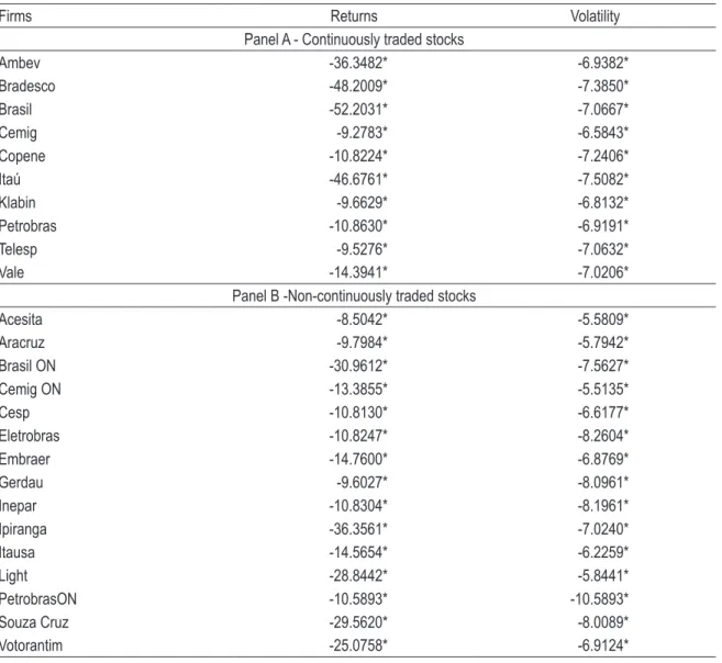
Table 1 presents the results for the unit root tests and evidence suggests that all series can be regarded as stationary as the null of a unit root is rejected in all cases for both stock returns and volatility with 1% significance level. Panels A and B, present results for a panel of 10 continuously traded stocks and non-continuously traded stocks, respectively.
5 In the end of 2001 the Brazilian stock exchange accounted for 45% total market capitalization for Latin America (Argentina, Peru, México and Chile).
6 It is important to notice that this introduces a bias as only the most liquid stocks enter the sample. 7 We fill in missing observations for these stocks using the closing price for the previous day.
table 1 – unit root adF tests
Firms Returns Volatility
Panel A - Continuously traded stocks
Ambev -36.3482* -6.9382*
Bradesco -48.2009* -7.3850*
Brasil -52.2031* -7.0667*
Cemig -9.2783* -6.5843*
Copene -10.8224* -7.2406*
Itaú -46.6761* -7.5082*
Klabin -9.6629* -6.8132*
Petrobras -10.8630* -6.9191*
Telesp -9.5276* -7.0632*
Vale -14.3941* -7.0206*
Panel B -Non-continuously traded stocks
Acesita -8.5042* -5.5809*
Aracruz -9.7984* -5.7942*
Brasil ON -30.9612* -7.5627*
Cemig ON -13.3855* -5.5135*
Cesp -10.8130* -6.6177*
Eletrobras -10.8247* -8.2604*
Embraer -14.7600* -6.8769*
Gerdau -9.6027* -8.0961*
Inepar -10.8304* -8.1961*
Ipiranga -36.3561* -7.0240*
Itausa -14.5654* -6.2259*
Light -28.8442* -5.8441*
PetrobrasON -10.5893* -10.5893*
Souza Cruz -29.5620* -8.0089*
Votorantim -25.0758* -6.9124*
Note: * Statistically significant at the 1% level.
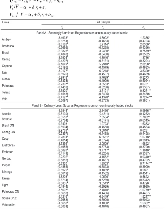
The next step is to estimate the relationship between risk and return and check the sign of the coefficients. Table 2 presents the results using SUR for 10 “continuously traded” stocks in Panel A,
and for 15 “non-continuously traded” stocks in Panel B.9 As we can see, the results are in line with
the findings of Duffee (1995). For all stocks, the coefficient d0 is significantly negative as in Black
(1976), Christie (1982) and Duffee (1995). Nonetheless, the coefficient d1 is significantly positive
implying a positive contemporaneous relation between stock returns and current volatility.
Eviden-ce on the d2 coefficient is much weaker.
table 2 – regressions of firm stock return volatility on firm stock returns, using dollar denomi-nated returns
(
Vt+1−Vt)
V = a + d + h0 0rt t+11 1
t t t
V V = a + d + εr
1 2 2 1
t t t
V+ V = a + d + υr +
Firms Full Sample
d0 d1 d2
Panel A - Seemingly Unrelated Regressions on continuously traded stocks
Ambev -3.4633*(0.6251) (0.4663)4.8902* (0.4703)1.2335*
Bradesco -3.3126*(0.5695) (0.4298)5.7114* (0.4366)2.0300*
Brasil -2.3823*(0.4848) (0.3488)3.2430* (0.3532)0.7579**
Cemig -3.3904*(0.4207) (0.3131)4.8046* (0.3204)1.3786*
Copene -2.1649*(0.6195) (0.4579)5.2948* (0.4633)2.8258*
Itaú -3.0177*(0.5976) (0.4597)6.9218* (0.4689)3.5390*
Klabin -5.9918*(0.6378) (0.4929)5.7629* -0.3273(0.5024)
Petrobras -3.2397*(0.4453) (0.3288)3.3553* (0.3307)0.0761
Telesp -2.6820*(0.4543) (0.3405)3.6121* (0.3430)0.8261**
Vale -3.4127*(0.5097) (0.3763)4.1370* (0.3801)0.7274***
Panel B - Ordinary Least Squares Regressions on non-continuously traded stocks
Acesita -1.3544*(0.5130) (0.4211)2.3466* (0.4232)0.9916**
Aracruz -5.6553*(0.7764) (0.6171)7.3504* (0.6315)1.7062*
Brasil ON -0.3403(0.5904) (0.4558)1.9723* (0.4563)1.6353*
Cemig ON -2.9763*(0.5397) (0.4438)3.6016* (0.4498)0.6281
Cesp -5.2861*(0.4814) (0.3724)6.3561* (0.3913)1.0718*
Eletrobras -3.7396*(0.4655) (0.3783)2.0509* -1.6892*(0.3790)
Embraer -2.5893*(0.4141) (0.3254)3.7717* (0.3337)1.1818*
Gerdau -2.2202*(0.5818) (0.4667)3.1552* (0.4702)0.9340**
Inepar -0.6320(0.4885) (0.3893)1.3503* (0.3900)0.7174***
Ipiranga -2.5979*(0.5619) (0.4502)3.1869* (0.4541)0.5891
Itausa -4.6208*(0.6714) (0.5289)4.0596* -0.5622(0.5342)
Light -3.0835*(0.4844) (0.3929)3.5543* (0.3985)0.4728
Petrobras ON -3.5607*(0.5653) (0.4436)2.4840* -1.0779**(0.4457)
Souza Cruz -5.1216*(0.7683) (0.5920)6.6449* (0.6043)1.5217**
Votorantim -1.5658*(0.6061) (0.4840)3.1030* (0.4867)1.5362*
Despite the significance of these coefficients we have found evidence of instability. Using
CUSUM test we have found evidence suggesting a structural break in 1994.10 We have also
perfor-med a CHOW test and a structural break could not be rejected for mid 1994.11 Hence, as a
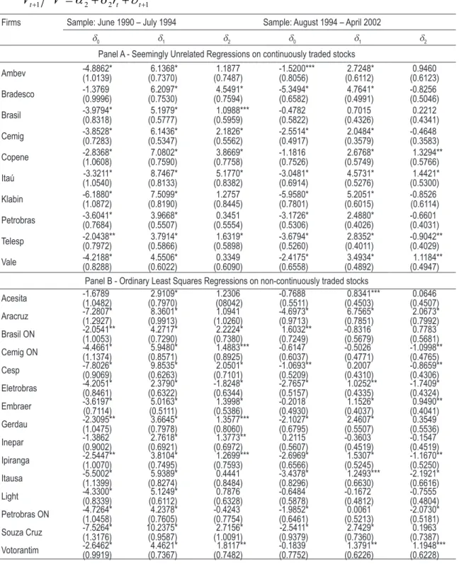
robust-ness check of the results we perform these SUR for two different sub-periods. The first sub-period begins in June 1990 and ends in July 1994 while the second begins in August 1994 and ends April 2002. Table 3 presents results for the two sub-periods analyzed. From the CUSUM test we infer that the coefficients are relatively stable for these sub-periods.
As we can see from Table 3, results are qualitatively the same indicating that when using dollar-denominated returns both periods show strong evidence supporting Duffee’s (1995) asser-tion.12
From Table 3 we can see that for all 10 “continuously traded” stocks the coefficients d0 have
a negative sign as found in previous studies such as in Black (1976), Christie (1982) and Duffee (1995). Even so, we have tested whether the primary reason for this negative relationship would be as suggested by Duffee (1995) that positive returns correspond to increases in current volatility. As
we can see, the sign of the d1 coefficients is significantly positive for all series, which suggest that
our sample behaves quite similarly to U.S. stocks. A qualitative similar result was obtained for the set of “non-continuously” traded stocks.
10 The break seems to be located in 1994. Therefore, we run our regressions with a dummy variable with value 0 prior to the break and 1 thereafter, defining the date of the break to be January, February, and so forth until August. We have chosen the date of the break as the date that maximizes the T-statistic for the dummy in these regressions, which was found to be for the period ending in July. This coincides with the introduction of the Stabilization Plan, denominated Real Plan, which was successful in bringing domestic inflation to a one-digit. Therefore, we have split the data in two sub-periods with a break in the end of July. 11 The CUSUM test is based on the cumulative sum of the recursive residuals. The test finds parameter instability if the cumula-tive sum goes outside the area between the two critical lines. See Brown et al. (1975) and Chow (1960) for a discussion on the CUSUM and Chow tests, respectively.
table 3 – regressions of firm stock return volatility on firm stock returns, using dollar denomi-nated returns
(
Vt+1−Vt)
V = a + d + h0 0rt t+11 1
t t t
V V = a + d + εr
1 2 2 1
t t t
V+ V = a + d + υr +
Firms Sample: June 1990 – July 1994 Sample: August 1994 – April 2002
d0 d1 d2 d0 d1 d2
Panel A - Seemingly Unrelated Regressions on continuously traded stocks
Ambev -4.8862*(1.0139) (0.7370)6.1368* (0.7487)1.1877 -1.5200***(0.8056) (0.6112)2.7248* (0.6123)0.9460
Bradesco -1.3769(0.9996) (0.7530)6.2097* (0.7594)4.5491* -5.3494*(0.6582) (0.4991)4.7641* -0.8256(0.5046)
Brasil -3.9794*(0.8318) (0.5777)5.1979* (0.5959)1.0988*** -0.4782(0.5822) (0.4326)0.7015 (0.4341)0.2212
Cemig -3.8528*(0.7283) (0.5347)6.1436* (0.5562)2.1826* -2.5514*(0.4917) (0.3579)2.0484* -0.4648(0.3583)
Copene -2.8368*(1.0608) (0.7590)7.0802* (0.7758)3.8669* -1.1816(0.7526) (0.5749)2.6768* (0.5766)1.3294**
Itaú (1.0540)-3.3211* (0.8133)8.7467* (0.8382)5.1770* -3.0481*(0.6914) (0.5276)4.5731* (0.5300)1.4421*
Klabin -6.1880*(1.0872) (0.8190)7.5099* (0.8445)1.2757 -5.9580*(0.7801) (0.6015)5.2051* -0.8526(0.6114)
Petrobras -3.6041*(0.7684) (0.5507)3.9668* (0.5554)0.3451 -3.1726*(0.5306) (0.4026)2.4880* -0.6601(0.4031)
Telesp -2.0438**(0.7972) (0.5866)3.7914* (0.5898)1.6319* -3.6794*(0.5260) (0.4011)2.8352* -0.9042**(0.4029)
Vale -4.2188*(0.8288) (0.6022)4.5506* (0.6090)0.3349 -2.4175*(0.6558) (0.4892)3.4934* (0.4947)1.1184**
Panel B - Ordinary Least Squares Regressions on non-continuously traded stocks
Acesita -1.6789(1.0482) (0.7970)2.9109* (08042)1.2306 -0.7688(0.5511) (0.4503)0.8341*** (0.4507)0.0646
Aracruz -7.2807*(1.2927) (0.9913)8.3601* (1.0260)1.0941 -4.6973*(0.9713) (0.7851)6.7565* (0.7992)2.0673*
Brasil ON -2.0541**(1.0053) (0.7290)4.2717* (0.7380)2.2224* (0.7249)1.6032** -0.8316(0.5679) (0.5681)0.7783
Cemig ON -4.4661*(1.1374) (0.8571)5.9480* (0.8925)1.4883*** -0.6147(0.6037) -0.5026(0.4771) -1.0998**(0.4765)
Cesp -7.8026*(0.9069) (0.6263)9.8535* (0.7101)2.0501* -1.0693**(0.5209) (0.4310)0.2007 -0.8659**(0.4306)
Eletrobras -4.2051*(0.8461) (0.6322)2.3790* -1.8248*(0.6344) -2.7657*(0.5157) (0.4335)1.0252** -1.7409*(0.4324)
Embraer -3.6197*(0.7114) (0.5111)5.0163* (0.5386)1.3998* -0.2018(0.4930) (0.4037)1.1526* (0.4041)0.9490**
Gerdau -2.3095**(1.0475) (0.7978)3.6645* (0.8060)1.3577*** -2.1027*(0.6795) (0.5507)2.4607* (0.5536)0.3549
Inepar -1.3862(0.9002) (0.6921)2.7618* (0.6972)1.3773** (0.5607)0.2115 -0.3603(0.4519) -0.1547(0.4519)
Ipiranga -2.5447**(1.0070) (0.7495)3.8104* (0.7593)1.2699*** -2.6969*(0.6566) (0.5245)1.5307* -1.1670**(0.5250)
Itausa -5.5002*(1.1399) (0.8274)5.9389* (0.8484)0.4441 -3.4378*(0.8296) (0.6630)1.2493*** -2.1921*(0.6616)
Light -4.3300*(0.8339) (0.6112)5.1249* (0.6328)0.7876 -0.6484(0.5878) -0.1672(0.4812) -0.7555(0.4804)
Petrobras ON -4.7264*(1.0458) (0.7605)4.2378* -0.4243(0.7754) -1.9852*(0.6461) (0.5213)0.0061 -2.0730*(0.5181)
Souza Cruz -7.5264*(1.3176) 10.2375*(0.9587) (1.0091)2.7156* (0.9379)-2.5411* (0.7360)2.7429* (0.7387)0.1963
Votorantim -2.6462*(0.9919) (0.7367)4.4621* (0.7482)1.8117** -0.1839(0.7752) (0.6226)1.3791** (0.6228)1.1948***
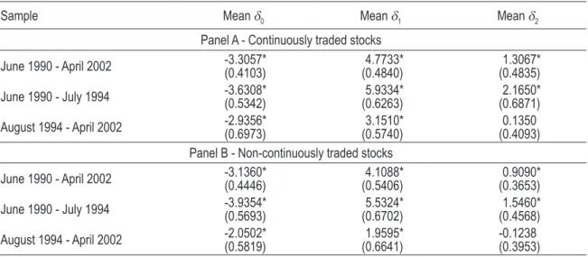
We turn next to analyze aggregate relationships between stock returns and volatility. Table 4 presents the results for the mean coefficients for the 10 stocks (Panel A) and uses the correc-ted standard error suggescorrec-ted in Duffee (1995). As we can see results are qualitatively the same for the entire sample and for both sub-periods suggesting that there is indeed a strong positive relationship between stock returns and current volatility. Furthermore, the results are qualita-tively the same for Panel B (“non-continuously traded” stocks).
table 4 – Summary of regressions of firm stock return volatility on firm stock returns
Sample Mean d0 Mean d1 Mean d2
Panel A - Continuously traded stocks
June 1990 - April 2002 -3.3057*(0.4103) (0.4840)4.7733* (0.4835)1.3067*
June 1990 - July 1994 -3.6308*(0.5342) (0.6263)5.9334* (0.6871)2.1650*
August 1994 - April 2002 -2.9356*
(0.6973)
3.1510* (0.5740)
0.1350 (0.4093) Panel B - Non-continuously traded stocks
June 1990 - April 2002 -3.1360*(0.4446) (0.5406)4.1088* (0.3653)0.9090*
June 1990 - July 1994 -3.9354*
(0.5693)
5.5324* (0.6702)
1.5460* (0.4568)
August 1994 - April 2002 -2.0502*
(0.5819)
1.9595* (0.6641)
-0.1238 (0.3953)
Note: * Rejection of the null with 1% level of significance. Standard errors are given in parenthesis.
From Table 4 we can see that the relationship between stock returns and future volatility is
not clear. In both continuously and non-continuously traded stocks samples the coefficient d2 is not
significant for the second sub-period, while it is significantly positive for the first sub-period and when using the entire sample, suggesting some instability. Nonetheless, the coefficient on current
volatility (d1) is significantly positive in all cases but is significantly smaller for the second
sub-pe-riod .
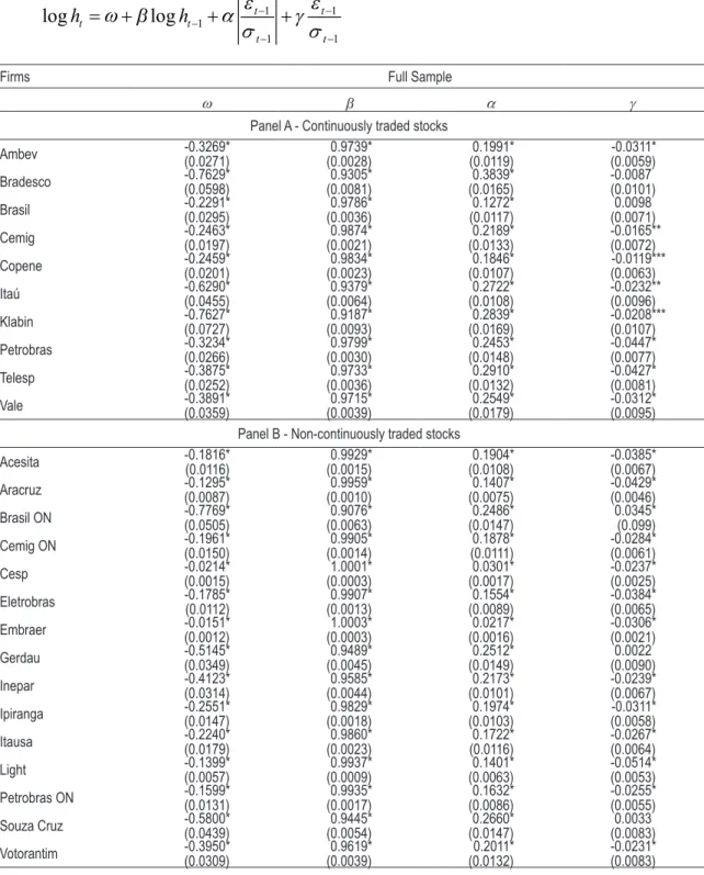
The next step is to present the AR(1)-EGARCH(1,1) estimation. It is important to notice that the leverage effect exists if and only if the distribution of the noise is left skewed. Thus, a leverage effect can be only generated by an asymmetrically distributed noise, which motivates the use of asymmetric ARCH models to test for the leverage effect. In Table 5 we show results for the entire period.
Residuals for some of these regressions seemed to have some degree of autocorrelation. We didn’t try to find the best model by the means of any information criteria but to estimate a
parsimo-nious model as suggested in the literature. Considering all 25 stocks we have that g is significantly
negative for over 80% of the firms. In only one case this coefficient is significantly positive and for four firms it is not significant. Thus, asymmetric effects on conditional volatility seem to be present
form in most stocks. A negative g implies that negative shocks to stock returns tend to have a larger
table 5 – ar(1)-eGarch(1,1) estimates for the 25 stocks sample
0 1 1
t t t
r = ϕ + ϕr− + υ , υ =t htεt, εt ~N
( )
0,1 ,1 1
1
1 1
log log t t
t t
t t
h h− − −
− −
ε ε
= w + b + a + g
σ σ
Firms Full Sample
w b a g
Panel A - Continuously traded stocks
Ambev -0.3269*(0.0271) (0.0028)0.9739* (0.0119)0.1991* (0.0059)-0.0311*
Bradesco -0.7629*(0.0598) (0.0081)0.9305* (0.0165)0.3839* -0.0087(0.0101)
Brasil -0.2291*(0.0295) (0.0036)0.9786* (0.0117)0.1272* (0.0071)0.0098
Cemig -0.2463*(0.0197) (0.0021)0.9874* (0.0133)0.2189* -0.0165**(0.0072)
Copene -0.2459*(0.0201) (0.0023)0.9834* (0.0107)0.1846* (0.0063)-0.0119***
Itaú -0.6290*(0.0455) (0.0064)0.9379* (0.0108)0.2722* -0.0232**(0.0096)
Klabin -0.7627*(0.0727) (0.0093)0.9187* (0.0169)0.2839* -0.0208***(0.0107)
Petrobras -0.3234*(0.0266) (0.0030)0.9799* (0.0148)0.2453* -0.0447*(0.0077)
Telesp -0.3875*(0.0252) (0.0036)0.9733* (0.0132)0.2910* -0.0427*(0.0081)
Vale -0.3891*(0.0359) (0.0039)0.9715* (0.0179)0.2549* -0.0312*(0.0095)
Panel B - Non-continuously traded stocks
Acesita -0.1816*(0.0116) (0.0015)0.9929* (0.0108)0.1904* -0.0385*(0.0067)
Aracruz -0.1295*(0.0087) (0.0010)0.9959* (0.0075)0.1407* -0.0429*(0.0046)
Brasil ON -0.7769*(0.0505) (0.0063)0.9076* (0.0147)0.2486* 0.0345*(0.099)
Cemig ON -0.1961*(0.0150) (0.0014)0.9905* (0.0111)0.1878* -0.0284*(0.0061)
Cesp -0.0214*(0.0015) (0.0003)1.0001* (0.0017)0.0301* -0.0237*(0.0025)
Eletrobras -0.1785*(0.0112) (0.0013)0.9907* (0.0089)0.1554* -0.0384*(0.0065)
Embraer -0.0151*(0.0012) (0.0003)1.0003* (0.0016)0.0217* -0.0306*(0.0021)
Gerdau -0.5145*(0.0349) (0.0045)0.9489* (0.0149)0.2512* (0.0090)0.0022
Inepar -0.4123*(0.0314) (0.0044)0.9585* (0.0101)0.2173* -0.0239*(0.0067)
Ipiranga -0.2551*(0.0147) (0.0018)0.9829* (0.0103)0.1974* (0.0058)-0.0311*
Itausa -0.2240*(0.0179) (0.0023)0.9860* (0.0116)0.1722* -0.0267*(0.0064)
Light -0.1399*(0.0057) (0.0009)0.9937* (0.0063)0.1401* -0.0514*(0.0053)
Petrobras ON -0.1599*(0.0131) (0.0017)0.9935* (0.0086)0.1632* -0.0255*(0.0055)
Souza Cruz -0.5800*(0.0439) (0.0054)0.9445* (0.0147)0.2660* (0.0083)0.0033
Votorantim -0.3950*(0.0309) (0.0039)0.9619* (0.0132)0.2011* -0.0231*(0.0083)
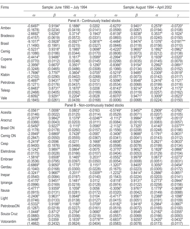
table 6 – ar(1)-eGarch(1,1) estimates for the 10 stocks sample
0 1 1
t t t
r = ϕ + ϕr− + υ , υ =t htεt, εt ~N
( )
0,1 ,1 1
1
1 1
log log t t
t t
t t
h h− − −
− −
ε ε
= w + b + a + g
σ σ
Firms Sample: June 1990 – July 1994 Sample: August 1994 – April 2002
w b a g w b a g
Panel A - Continuously traded stocks
Ambev -0.6497*(0.1678) (0.0234)0.9194* (0.0419)0.1886* (0.0141)0.0202 -0.6270*(0.0599) (0.0067)0.9401* (0.0194)0.2578* -0.0720*(0.0108)
Bradesco -2.6692*(0.4157) (0.0619)0.6250* (0.0572)0.3714* (0.0331)0.1943* -0.8139*(0.0893) (0.0113)0.9238* (0.0240)0.3537* -0.1024*(0.0150)
Brasil -9.1017*(1.1490) -0.5928*(0.1991) -0.0921**(0.0215) (0.0327)0.0816** -0.4484*(0.0848) (0.0118)0.9474* (0.0156)0.1376* -0.0181***(0.0110)
Cemig -0.5231*(0.1086) (0.0186)0.9318* (0.0344)0.1985* (0.0170)0.0698* -0.4220*(0.0608) (0.0073)0.9600* (0.0212)0.1892* -0.0962*(0.0138)
Copene -0.4414*(0.0770) (0.0112)0.9486* (0.0246)0.1617* (0.0145)0.0589* -0.2994*(0.0299) (0.0035)0.9779* (0.0145)0.1939* -0.0320*(0.0079)
Itaú -2.3956*(0.3248) (0.0465)0.6670* (0.0486)0.3501* (0.0308)0.1290* -0.8366*(0.1066) (0.0134)0.9154* (0.0260)0.2992* -0.0891*(0.0152)
Klabin -1.7696*(0.2102) (0.0290)0.7797* (0.0402)0.3804* (0.0268)0.0705* -0.5219*(0.0577) (0.0073)0.9485* (0.0142)0.2309* -0.0519*(0.0117)
Petrobras -0.4697*(0.1271) (0.0176)0.9431* (0.0437)0.1760* (0.0151)0.0210 -0.5096*(0.0534) (0.0068)0.9548* (0.0199)0.2416* -0.1121*(0.0116)
Telesp -0.8483*(0.2468) (0.0405)0.8731* (0.0392)0.1870* (0.0189)0.0208 -0.8143*(0.0909) (0.0119)0.9214* (0.0257)0.3514* (0.0162)-0.1172*
Vale -0.6092*(0.1845) (0.0261)0.9291* (0.0439)0.2204* (0.0168)-0.0028 -0.6070*(0.0006) (0.0068)0.9471* (0.0224)0.3009* -0.0523*(0.0150)
Panel B - Non-continuously traded stocks
Acesita -0.0561*(0.0146) (0.0022)1.0006* (0.0125)0.0803* (0.0114)-0.0163 -0.5749*(0.0529) (0.0071)0.9457* (0.0207)0.2909* -0.0760*(0.0105)
Aracruz -0.2079*(0.0366) (0.0043)0.9842* (0.0203)0.1379* -0.0246**(0.0111) (0.0084)-0.1112* (0.0010)0.9984* (0.0083)0.1385* -0.0513*(0.0057)
Brasil ON -0.5450*(0.1178) (0.0178)0.9227* (0.0260)0.1115* (0.0157)0.0580* (0.1556)-2.1132* (0.0208)0.7325* (0.0248)0.4140* (0.0186)0.0377**
Cemig ON -2.0949*(0.2847) (0.0550)0.6869* (0.0555)0.7428* (0.0367)-0.0587 -0.3406*(0.0341) (0.0041)0.9688* (0.0143)0.1791* -0.0631*(0.0112)
Cesp -5.2419*(0.9400) -0.0596(0.1876) (0.0466)-0.0211 (0.0459)0.1668* -0.6608*(0.0598) (0.0078)0.9264* (0.0199)0.2621* -0.0633*(0.0134)
Eletrobras -0.1242*(0.0175) (0.0028)0.9897* (0.0166)0.0864* (0.0107)-0.0075 -0.3770*(0.0404) (0.0053)0.9652* (0.0129)0.1828* -0.0866*(0.0104)
Embraer -1.5816*(0.3536) (0.0795)0.6508* (0.0397)0.1465* (0.0350)0.2031* -0.0552*(0.0054) (0.0008)0.9979* (0.0051)0.0673* -0.0273*(0.0031)
Gerdau -0.6869*(0.1040) (0.0168)0.9050* (0.0300)0.1770* (0.0228)0.1151* -1.3207*(0.1675) (0.0223)0.8405* (0.0305)0.3050* -0.0454*(0.0172)
Inepar -0.3241*(0.0540) (0.0084)0.9687* (0.0197)0.2011* (0.0140)0.0309** -1.2232*(0.1543) (0.0224)0.8414* (0.0203)0.2886* -0.0651*(0.0141)
Ipiranga -0.4170*(0.0996) (0.0169)0.9451* (0.0218)0.1481* (0.0128)0.0112 (0.0974)-0.8118* (0.0122)0.9131* (0.0258)0.2773* -0.0944*(0.0156)
Itausa -0.4771*(0.0915) (0.0131)0.9359* (0.0281)0.1058* (0.0172)0.0056 -0.3056*(0.0320) (0.0042)0.9761* (0.0149)0.1779* -0.0608*(0.0088)
Light -0.2406*(0.0746) (0.0133)0.9631* (0.0138)0.0648* (0.0127)0.0104 -0.4717*(0.0415) (0.0051)0.9561* (0.0191)0.2388* -0.1098*(0.0109)
PetrobrasON -0.5332*(0.1287) (0.0218)0.9188* (0.0227)0.1180* (0.0161)0.0709* -0.6182*(0.0519) (0.0072)0.9416* (0.0165)0.2984* -0.0667*(0.0100)
Souza Cruz -1.0448*(0.0880) (0.0129)0.8712* (0.0356)0.2764* (0.0218)0.0680* -0.4861*(0.0557) (0.0069)0.9546* (0.0166)0.2182* -0.0355*(0.0093)
Votorantim -5.9498*(1.4662) (0.2432)0.0359 (0.0624)0.1835* (0.0404)0.0778*** -0.6837*(0.0583) (0.0078)0.9255* (0.0173)0.2420* -0.0432*(0.0117)
Table 6 presents results for the two sub-periods analyzed. Residuals for these regressions look much nicer than before. As we can see the leverage coefficient is significant for all stocks and when testing for all 25 stocks we find that for 96% of the firms this coefficient is significantly negative for the second sub-sample, a result that is in line with the findings of Cheung and Ng (1992).
The log-likelihood statistics are large for both sub-periods suggesting that the AR(1)-EGAR-CH(1,1) is a fair representation of daily returns. The EGARCH parameter is statistically significant
for all stocks. In both tables the b coefficients are considerably larger than a, which implies that
large market surprises induce relatively small revisions in future volatility.
We have also run AR(1)-E-GARCH(1,1)-M estimation and found evidence in line with pre-vious studies for the U.S. and industrialized countries which have found that the standard devia-tion in the mean equadevia-tion is not significant.13
A problem with the previous estimations is that the covariance stationarity condition a + b << 1 is not satisfied. Engle and Ng (1993) propose a test to check whether positive and nega-tive shocks have a different impact on conditional variance. Let It−−1 be a dummy variable with
value 1 when the error term for a model for the conditional mean is negative and 0 otherwise. The test can be implemented as follows
2
0 1 1
ˆ It−− t
ε = ϕ + ϕ + h (3a)
2
0 2 1 1
ˆ It−− ˆt− t
ε = ϕ + ϕ ε + h (3b)
2
0 3 1 1
ˆ It+− ˆt− t
ε = ϕ + ϕ ε + h (3c)
2
0 1 1 2 1 1 3 1 1
ˆ It−− It−− ˆt− It+− ˆt− t
ε = ϕ + ϕ + ϕ ε + ϕ ε + h (3d)
where It+−1= −1 It−−1.
The sign bias (SB) tests whether ϕ =1 0, i.e., if the magnitude of the current shock depends
on the sign of the lagged shock. By testing ϕ =2 0 and ϕ =3 0 we examine whether the effect of
negative (negative size bias NSB) or positive (positive size bias PSB) shocks on the conditional va-riance also depend on their size.
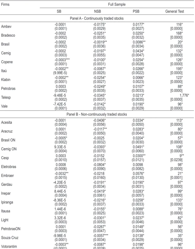
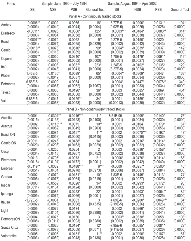
Tables 7 and 8 present results for the SB. There is clearly an asymmetric ARCH effect for the full sample and also for the August-1994/April-2002 sub-period. If we compare the statistics of the SB tests with those of the NSB and PSB the size effects appear to be more important than sign effects.
table 7 – Sign bias, negative size bias, positive size bias and general test
Firms Full Sample
SB NSB PSB General Test
Panel A - Continuously traded stocks
Ambev -0.0001(0.0001) -0.0175*(0.0029) (0.0027)0.0177* [0.0000]116*
Bradesco -0.0002(0.0002) -0.0251*(0.0035) (0.0032)0.0250* [0.0000]168*
Brasil -0.0002(0.0002) -0.0019**(0.0036) (0.0034)0.0086** [0.0000]20*
Cemig -0.0002(0.0003) -0.0197*(0.0055) (0.0047)0.0434* [0.0000]132*
Copene -0.0003***(0.0001) -0.0100*(0.0031) (0.0028)0.0254* [0.0000]126*
Itaú (9.99E-5)-0.0002** -0.0067*(0.0025) (0.0022)0.0266* [0.0000]195*
Klabin -0.0002**(0.0001) -0.0254*(0.0027) 0.0066*0.0023) [0.0000]123*
Petrobras (0.0002)0.0003 -0.0249*(0.0035) (0.0033)0.0107* [0.0000]88*
Telesp -9.48E-5(0.0002) -0.0345*(0.0037) (0.0035)0.0213* [0.0000]1,776*
Vale -7.42E-5(0.0001) -0.0142*(0.0032) (0.0029)0.0190* [0.0000]96*
Panel B - Non-continuously traded stocks
Acesita -0.0001(0.0004) -0.0406*(0.0056) (0.0050)0.0334* [0.0000]113*
Aracruz (0.0002)0.0001 (0.0050)-0.0117** (0.0040)0.0283* [0.0000]80*
Brasil ON -0.0005*(0.0002) -0.0025(0.0032) (0.0030)0.0204* [0.0000]57*
Cemig ON 9.33E-5(0.0004) -0.0393*(0.0070) (0.0060)0.0491* [0.0000]108*
Cesp (0.0010)0.0003 -0.0152(0.0157) (0.0121)0.0300** [0.0239]9**
Eletrobras (0.0006)0.0008 -0.0804*(0.0090) (0.0082)0.0098 [0.0000]98*
Embraer -0.0032**(0.0015) -0.0218(0.0160) (0.0130)0.0576* [0.0001]21*
Gerdau -4.20E-5(0.0002) -0.0191*(0.0034) (0.0031)0.0190* [0.0000]97*
Inepar 8.44E-5(0.0004) -0.0419*(0.0061) (0.0057)0.0283* [0.0000]99*
Ipiranga -8.36E-5(0.0002) -0.0216*(0.0037) (0.0033)0.0258* [0.0000]133*
Itausa 1.44E-6(0.0001) -0.0155*(0.0025) (0.0023)0.0088* [0.0000]76*
Light 3.32E-6(0.0003) -0.0301*(0.0053) (0.0046)0.0237* [0.0000]82*
PetrobrasON (0.0003)0.0001 -0.0267*(0.0047) (0.0044)0.0148* [0.0000]56*
Souza Cruz -9.98E-5(0.0001) -0.0057***(0.0034) (0.0029)0.0138* [0.0000]35*
Votorantim ((0.0001)-0.0003** -0.0087*(0.0028) (0.0025)0.0198* [0.0000]96*
Notes: The *, ** and *** denote statistically significance at the 1%, 5% and 10% level, respectively and standard errors are given in parenthesis.
table 8 – Sign bias, negative size bias, positive size bias and general test
Firms Sample: June 1990 – July 1994 Sample: August 1994 – April 2002
SB NSB PSB General Test SB NSB PSB General Test
Panel A - Continuously traded stocks
Ambev -0.0006**(0.0003) (0.0049)0.0002 (0.0044)0.0065 [0.0004]18* (9.02E-5)3.77E-5 -0.0206*(0.0025) (0.0026)0.0131* [0.0000]194*
Bradesco (0.0003)-0.0011* (0.0064)0.0023 (0.0058)0.0368* [0.0000]125* (0.0001)0.0003*** -0.0484*(0.0038) (0.0037)0.0083** [0.0000]314*
Brasil -0.0007***(0.0004) (0.0074)0.0070 (0.0055)0.0062 [0.0329]9** 9.27E-5(0.0002) -0.0150*(0.0042) (0.0043)0.0020 [0.0000]26*
Cemig -0.0018**(0.0008) (0.0113)0.0076 (0.0089)0.0510* [0.0000]99* (0.0002)0.0004** -0.0339*(0.0039) (0.0039)0.0037 [0.0000]142*
Copene -0.0007**(0.0003) (0.0063)0.0050 (0.0052)0.0310* [0.0000]107* 1.70E-5(0.0001) -0.0179*(0.0027) (0.0027)0.0091* [0.0000]119*
Itaú -0.0007*(0.0002) (0.0048)0.0006 (0.0041)0.0352* [0.0000]223* (8.27E-5)1.24E-5 -0.0102*(0.0024) (0.0023)0.0135* [0.0000]129*
Klabin 1.46E-5(0.0002) -0.0135*(0.0049) 0.0099*0.0037) [0.0000]65* -0.0004**(0.0001) -0.0309*(0.0034) (0.0030)0.0047 [0.0000]163*
Petrobras -6.56E-5(0.0004) (0.0067)0.0009 (0.0062)0.0034 [0.7967]1 (0.0001)0.0004* -0.0447*(0.0033) (0.0034)0.0078** [0.0000]340*
Telesp -0.0006(0.0005) -0.0005(0.0063) (0.0058)0.0190* [0.0000]36* (0.0002)0.0003 -0.0685*(0.0044) (0.0044)0.0069 [0.0000]454*
Vale 6.86E-5(0.0003) -0.0047(0.0058) (0.0053)0.0129** [0.0000]34* (0.00013)-0.0001 -0.0159*(0.0035) (0.0032)0.0186* [0.0000]126*
Panel B - Non-continuously traded stocks
Acesita -0.0001(0.0015) -0.0304**(0.0136) (0.0123)0.0216*** [0.0100]11* 8.51E-05(0.0001) -0.0209*(0.0034) (0.0030)0.0140* [0.0000]76*
Aracruz (0.0002)0.0002 (0.0062)-0.0115*** (0.0049)0.0075 [0.0203]10** (0.0003)0.0001 -0.0104(0.0069) (0.0056)0.0379* [0.0000]67*
Brasil ON -0.0009*(0.0003) (0.0058)0.0084 (0.0050)0.0157* [0.0115]11** -0.0002(0.0002) -0.0070***(0.0036) (0.0036)0.0192* [0.0000]43*
Cemig ON (0.0020)-0.0011 -0.0246(0.0206) (0.0163)0.0488* [0.0029]14* (0.0002)0.0002 -0.0216*(0.0032) (0.0032)0.0114* [0.0000]64*
Cesp -0.0004(0.0034) (0.0413)0.0250 (0.0267)0.0254 [0.6752]2 (0.0002)0.0003 -0.0336*(0.0038) (0.0037)0.0158* [0.0000]124*
Eletrobras (0.0018)0.0013 -0.0795*(0.0191) -0.0073(0.0172) [0.0001]21* (0.0002)0.0006* -0.0476*(0.0042) (0.0040)0.0114* [0.0000]168*
Embraer (0.0051)-0.0119** (0.0404)0.0332 (0.0278)0.0488*** [0.0973]6*** -0.0009(0.0006) -0.0257*(0.0087) (0.0084)0.0500* [0.0000]40*
Gerdau -0.0002(0.0005) -0.0079(0.0073) (0.0064)0.0151** [0.0219]10** -7.83E-5(0.0001) -0.0145*(0.0027) (0.0025)0.0113* [0.0000]74*
Inepar -0.0003(0.0011) -0.0559*(0.0134) (0.0124)0.0328* [0.0000]34* (0.0002)0.0002 -0.0293*(0.0042) (0.0041)0.0172* [0.0000]93*
Ipiranga -0.0005(0.0005) -0.0085(0.0074) (0.0066)0.0253* [0.0001]22* (0.0001)0.0001 -0.0203*(0.0027) (0.0025)0.0064** [0.0000]82*
Itausa -1.72E-5(0.0002) -0.0031(0.0046) (0.0008)0.0003 [0.4335]3 (9.19E-5)4.69E-6 -0.0200*(0.0026) (0.0026)0.0049*** [0.0000]84*
Light -0.0005(0.0008) -0.0072(0.0104) (0.0086)0.0134 [0.2288]4 (0.0002)0.0002 -0.0266*(0.0041) (0.0041)0.0143* [0.0000]73*
PetrobrasON -0.0004(0.0008) -0.0075(0.0111) (0.0093)0.0130 [0.3280]3 (0.0002)0.0003** -0.0338*(0.0035) (0.0035)0.0058 [0.0000]108*
Souza Cruz -0.0003(0.0003) (0.0073)0.0026 (0.0059)0.0194* [0.0071]12* -7.95E-6(9.11E-5) -0.0085*(0.0027) (0.0026)0.0081* [0.0000]29*
Votorantim -0.0005(0.0003) (0.0052)0.0008 (0.0043)0.0131* [0.0136]11** -0.0002(0.0001) -0.0090*(0.0030) (0.0028)0.0187* [0.0000]67*
Notes: The *, ** and *** denote statistically significance at the 1%, 5% and 10% level, respectively and standard errors are given in parenthesis.
5 F
irMSizeandleveraGeFor all firms we have calculated the mean debt/equity ratio, market capitalization and total assets as a proxy for firm size for the entire period and for the August 1994 April 2002 sub-period.
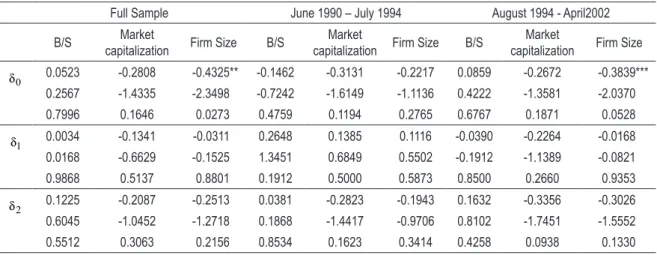
We have used Spearman rank correlation (nonparametric statistic) to check whether the mag-nitude of the coefficients in the regressions relating volatility and stock returns were related to these variables. Table 9 presents empirical results. All 25 stocks were included in the analysis.
table 9 – Spearman rank correlations
Full Sample June 1990 – July 1994 August 1994 - April2002
B/S Market
capitalization Firm Size B/S
Market
capitalization Firm Size B/S
Market
capitalization Firm Size
0
δ 0.0523 -0.2808 -0.4325** -0.1462 -0.3131 -0.2217 0.0859 -0.2672 -0.3839***
0.2567 -1.4335 -2.3498 -0.7242 -1.6149 -1.1136 0.4222 -1.3581 -2.0370
0.7996 0.1646 0.0273 0.4759 0.1194 0.2765 0.6767 0.1871 0.0528
1
δ 0.0034 -0.1341 -0.0311 0.2648 0.1385 0.1116 -0.0390 -0.2264 -0.0168
0.0168 -0.6629 -0.1525 1.3451 0.6849 0.5502 -0.1912 -1.1389 -0.0821
0.9868 0.5137 0.8801 0.1912 0.5000 0.5873 0.8500 0.2660 0.9353
2
δ 0.1225 -0.2087 -0.2513 0.0381 -0.2823 -0.1943 0.1632 -0.3356 -0.3026
0.6045 -1.0452 -1.2718 0.1868 -1.4417 -0.9706 0.8102 -1.7451 -1.5552
0.5512 0.3063 0.2156 0.8534 0.1623 0.3414 0.4258 0.0938 0.1330
Notes: B/S stands for debt to equity ratio, the ** and *** denote statistically significance at the 5% and 10% level, respec-tively.
Obs: In the first row we present the Spearman rank correlations, in the second row the t-statistic and in the last row the p-value.
For most cases these correlations were not significant for both the entire sample and for the
second sub-period. Only for g0 and firm size we find evidence of a relationship for the entire period
at the 5% significance level and at the 10% significance level for the latter sub-period.
This suggests that there could be other elements driving results and further analysis is left for future research.
6 c
oncluSionSIn this paper we have tested the relationship between stock returns and current and future volatility. In line with the findings of Cheung and Ng (1992) and Duffee (1995) we have found evi-dence suggesting that stock returns are significantly related to current volatility while the relation with future volatility is much weaker.
as the major cause of instability. Therefore, we have presented results for the period prior to July 1994 and afterwards.
Evidence presented using both a SUR methodology and an AR(1)-EGARCH(1,1) estimation suggests that changes in volatility are negatively related to stock returns, a result that has been found in the literature examining this relationship since Black (1976). Evidence from the Engle and Ng (1993) test clearly indicates that there are asymmetric ARCH effects. Many explanations have been given for this phenomenon.
Duffee (1995) has argued that this relationship has been found to be negative due to a positive relation between current volatility and stock returns. This test has been applied to 25 Brazilian stocks (which are highly representative) and we found evidence that Duffee’s hypothesis cannot be rejected.
We have finally used Spearman rank correlation (nonparametric statistic) to check whether the magnitude of the coefficients in the regressions relating volatility and stock returns were related to variables such as firm size (measured by market capitalization and total assets) and debt/equity ratios. These correlations were not significant for the entire sample and for sub-periods analyzed.
The empirical results found in this paper have important implications for volatility forecas-ting. We have found strong asymmetric effects in volatility, which implies that asymmetric-GAR-CH models are to be preferred to usual GARasymmetric-GAR-CH models for portfolio and risk management, and also for building models for pricing assets and derivatives.
The relationship between returns and volatility has been explained in the financial literature by viewing stocks as options on the assets of the firm, which implies that higher debt/equity ratios should exhibit stronger negative lagged correlations between stock returns and volatility (see Black (1976) and Christie (1982). Our empirical results are inconsistent with this implication.
Further analysis on these issues is crucial. An interesting extension of this paper would be to use local currency-denominated returns and tests for exchange rate effects on the results. Finally, augmenting the sample and exploring more in depth issues of infrequent trading and the implica-tions on the results obtained would be an interesting line for further research.
r
eFerenceSANDERSEN, T. G.; BOLLERSLEV, T.; CAI, J. Intraday and interday volatility in the Japanese stock market. Journal of international Financial Markets, institutions and Money, v. 10, p. 107-130, 2000. BLACK, F. Studies of stock price volatility changes. Proceedings of the 1976 meetings of the American
Statistical Association, Business and Economics Statistics Section. Washington, DC: American Sta-tistical Association, p. 177-181, 1976.
BROWN, R. L.; DURBIN, J.; EVANS, J. M. Techniques for testing the constancy of regression relation-ships over time. Journal of the Royal Statistical Society, v. 37, p. 149-192, 1975.
CHEUNG, Yin-Wong; NG, Lilian K. Stock price dynamics and firm size: an empirical investigation.
The Journal of Finance, v. 47, p. 1985-1997, 1992.
CHRISTIE, A. The stochastic behavior of common stock variances: value, leverage, and interest rate ef-fects. Journal of Financial Economics, v. 10, p. 407-432, 1982.
DE SANTIS, G.; IMROHOROGLU, S. Stock returns and volatility in emerging financial markets. Journal
of international Money and Finance, v. 16, p. 561-579, 1997.
DICKEY, D. A.; FULLER, W. A. Likelihood ratio statistics for autoregressive time series with a unit root.
Econometrica, v. 49, p. 1057-1072, 1981.
DUFFEE, G. Stock return and volatility: A firm level analysis. Journal of Financial Economics, v. 37, p. 399-420, 1995.
ENGLE, R. F.; GALLO, G. M. Multiple indicators model for volatility using intra-daily data, Journal of
Econometrics, v. 131, p. 3-27, 2006.
________.; NG, V. K. Measuring and testing the impact of news on volatility. The Journal of Finance, v. 48, p. 1749-1778, 1993.
FRENCH, K. R.; SCHWERT, G. W.; STAMBAUGH, R. F. Expected stock returns and volatility. Journal
of Financial Economics, v. 19, p. 3-29, 1987.
GHYSELS, E.; SANTA-CLARA, P.; VALKANOV, R. Predicting volatility: getting the most out of return data sampled at different frequencies. Journal of Econometrics, v. 131, p. 59-95, 2006.
JUNGBACKER, B.; KOOPMAN, S. J. Model-based measurement of actual volatility in high-frequency data. advances in Econometrics, v. 20, p. 183-210, 2006.
KENDALL, M. G. Rank correlation methods. New York: Griffin, 1962.
LI, Q.; YANG, J.; HSIAO, C.; YOUNG-JAE, C. The relationship between stock returns and volatility in international stock markets. Journal of Empirical Finance, v. 12, p. 650-665, 2005.
MARTENS, M.; VAN DIJK, D. Measuring volatility with the realized range. Journal of Econometrics, v. 138, p. 181-207, 2007.
MARKOWITZ, H. Potfolio selection. Journal of Finance, v. 7, 77-91, 1952.
MOUGOUÉ, M.; WHYTE, A. M. Stock returns and volatility: an empirical investigation of the German and French equity markets. Global Finance Journal, v. 7, p. 253-263, 1996.
NELSON, D. B. Conditional heteroskedasticity in asset returns: a new approach. Econometrica, v. 59, p. 347-370, 1991.
NG, S; Perron, P. Unit roots tests in ARMA models with data dependent methods for the selection of the truncation lag. Journal of the americam statistical association, v. 90, p. 268-281, 1995.
________. Lag length selection and the construction of unit roots tests with good size and power.
Econo-metrica, v. 69, p. 1519-1554, 2001.
THEODOSSIOU, P.; LEE, U. Relationship between volatility and expected returns across international stock markets. Journal of Business Finance & accounting, v. 22, p. 289-300, 1995.
