Universidade de Aveiro 2012
Departamento de Biologia
Tânia Marisa
Neves Mendes
Avaliação
integrada
de
rios
baseada
em
diatomáceas e macroinvertebrados
Combined assessment of streams based on diatoms
and macroinvertebrates
Dissertação apresentada à Universidade de Aveiro para cumprimento dos requisitos necessários à obtenção do grau de Mestre em Ecologia, Biodiversidade e Gestão de Ecossistemas, realizada sob a orientação científica da Doutora Salomé Fernandes Pinheiro de Almeida, Professora Auxiliar do Departamento de Biologia da Universidade de Aveiro e da Doutora Maria João de Medeiros Brazão Lopes Feio, Investigadora Auxiliar do Instituto do Mar da Universidade de Coimbra.
Dedico este trabalho ao meu pai. I dedicate this work to my father.
o júri / the jury
Presidente / president Doutor João António de Almeida Serôdio
Professor Auxiliar do Departamento de Biologia da Universidade de Aveiro
Vogais / examiners committee Doutor Bruce Chessman
Principal Research Scientist at the New South Wales Office of Environment and Heritage
Doutora Salomé Fernandes Pinheiro de Almeida
Professora Auxiliar do Departamento de Biologia da Universidade de Aveiro (orientadora)
Doutora Maria João de Medeiros Brazão Lopes Feio
agradecimentos / acknowledments
A realização desta dissertação não teria sido possível sem a ajuda de várias pessoas.
Em primeiro lugar agradeço à Professora Doutora Salomé Almeida (orientadora) e à Doutora Maria João Feio (co-orientadora) pela ajuda, orientação e conhecimento transmitido ao longo da minha dissertação e também pela amizade e disponibilidade demonstradas.
À Carmen Elias, Sónia Serra, Ana Calapez e à Ana Luís por toda a ajuda disponibilizada durante as saídas de campo e no laboratório. Obrigada pela amizade, apoio e paciência.
Agradeço a dois amigos especiais, Raquel Silva e Luís Matos, os quais permaneceram sempre do meu lado.
Luís, obrigada por toda a paciência, dedicação, apoio e motivação em todos os momentos.
Por fim, um enorme obrigado à minha família pelo apoio incondicional e porque sem eles jamais teria chegado até aqui.
Palavras chave Modelos preditivos, diatomáceas, macroinvertebrados, Directiva Quadro da Água, rios, biomonitorização
Resumo As diatomáceas e os macroinvertebrados fornecem informação complementar na avaliação da qualidade da água. No entanto, os métodos utilizados para esse fim têm sido desenvolvidos separadamente para as duas comunidades. O objetivo deste estudo foi verificar se um modelo preditivo baseado nos dois elementos biológicos produz uma avaliação mais simplista e simultaneamente mais holística e robusta da qualidade dos ecossistemas face aos métodos individuais, os quais necessitam de ser combinados posteriormente, usualmente com base na abordagem “one-out al-out”. Para tal, foram utilizados dois métodos, RIVPACS e BEAST, devido às suas diferentes características, especialmente porque o RIVPACS utiliza dados de presença/ausência enquanto o BEAST utiliza dados de abundância. Foram construídos 6 modelos preditivos para o território português: dois para as diatomáceas, dois para os macroinvertebrados e dois integrando as duas comunidades. Nas primaveras de 2004 e 2005 foram simultaneamente amostradas diatomáceas e macroinvertebrados de 143 locais minimamente perturbados. Foram selecionados 23 locais afetados por contaminação orgânica, efluentes industriais e minas do centro de Portugal para serem utilizados como locais teste. O modelo RIV INV+DIAT atribuiu a mesma classe de qualidade do que o método “one-out all-out” a cerca de 70% dos locais teste, enquanto o BEAST INV+DIAT apenas partilhou cerca de 40% dos locais com a mesma classe. As respostas dos diferentes métodos (incluindo o “one-out all-out”) à degradação ambiental foram avaliadas através de correlações de Spearman. Apesar do RIVPACS ser menos sensível do que o BEAST, demonstrou funcionar melhor quando se combinam as duas comunidades. O tipo de dados influenciou a avaliação dos dois métodos demonstrando ser apenas fiável integrar as diatomáceas e os macroinvertebrados num único método usando dados de presença/ausência.
keywords Predictive models, diatoms, macroinvertebrates, Water Framework Directive, streams, bioassessment
abstract Diatoms and macroinvertebrates provide complementary information on stream water quality. However, classification methods have been developed separately for the two biological elements. The aim of the present study was to assess if a predictive model based on the evaluation of biodiversity using taxa from both biological elements, produces a simpler and simultaneously more holistic and accurate assessment of stream health than individual methods. These classifications need to be combined later, usually based on “one-out all-out” approach. For that purpose, two different approaches were used, BEAST and RIVPACS, due to their different characteristics, mostly because RIVPACS uses presence/absence data while BEAST uses abundance. Six predictive models were built for the entire Portuguese territory: two for diatoms, two for macroinvertebrates and two combining diatom and macroinvertebrate communities. Data from 143 minimally disturbed sites sampled simultaneously for diatoms and invertebrates in the spring of 2004 and 2005 were used to calibrate and validate the models. For all the six predictive models, 23 impacted streams from central Portugal affected by organic contamination, industrial effluents and mine drainage were used as test sites. The RIV INV+DIAT model shared with “one-out all-out” approach about 70% of the test sites with the same quality class while the BEAST INV+DIAT model only shared about 40%. The responses to the environmental degradation of the different approaches (including the “one-out all-out”) were analyzed through a Spearman correlation. In spite of the less sensitive RIVPACS approach results in comparison to BEAST, it showed to work better when the two biological elements were joined. The type of data influenced the assessment of the two approaches and diatoms and macroinvertebrates can be integrated reliably into a single method using only the presence/absence type of data.
Index
Index of Figures ... iii
Index of Tables ... v
Acronym list ... vii
Chapter 1 - INTRODUCTION ...1
1.1 Macroinvertebrates as bio-indicators of water quality ...2
1.2 Diatoms as bio-indicators of water quality ...5
1.3 Predictive Models overview ...8
1.3.1 RIVPACS approach ... 10
1.3.2 BEAST approach ... 12
1.4 Goals ... 14
Chapter 2 – STUDY AREA ...17
2.1 Test site characterization ... 19
2.1.1 Botão (M18) ... 19 2.1.2 Foz do Alva (M55) ... 20 2.1.3 Lousã-Piscinas (M2002) ... 20 2.1.4 Lousã-Fábrica do Papel (M101)... 21 2.1.5 Foz do Ceira (M2001) ... 22 2.1.6 Lorvão (M108) ... 22 2.1.7 Casal do Ermio (M109) ... 23
2.1.8 Nossa Senhora da Piedade de Tábua (M112) ... 24
2.1.9 Miranda do Corvo 3 (M111) ... 24
2.1.10 Miranda do Corvo (M110) ... 25
2.1.11 Covão dos Mendes/Crespos (M43) ... 26
2.1.12 Cunha Baixa (M123) ... 26
2.1.13 Casal da Misarela (M49) ... 27
2.1.14 Urgeiriça (M122) ... 28
2.1.15 Mogofores (V78) ... 28
2.1.16 Vila Verde (V94)... 29
2.1.17 São João da Madeira (V125) ... 30
2.1.18 Travanca (V124) ... 30 2.1.19 Alfusqueiro (V36)... 31 2.1.20 Carvalhal (V118) ... 31 2.1.21 Estarreja (V119) ... 32 2.1.22 Colmeias (L42) ... 33 2.1.23 Chãs (L120) ... 33 Chapter 3 – METHODS ...35 3.1 Data base ... 35 3.2 Biological data ... 35
3.3 Abiotic data ... 38
3.4 Data analysis ... 41
3.4.1 Models building ... 41
3.4.2 Classification system ... 43
3.4.3 Models validation and testing ... 43
3.4.4 Response to pressures ... 44
Chapter 4 – RESULTS ...45
4.1 RIV DIAT model ... 45
4.2 RIV INV model ... 51
4.3 RIV INV+DIAT model ... 56
4.4 BEAST DIAT model ... 63
4.5 BEAST INV model ... 66
4.6 BEAST INV+DIAT model ... 71
4.7 Assessment of test sites ... 76
Chapter 5 – DISCUSSION and CONCLUSIONS ...93
REFERENCES ... 101
Appendix A – List of reference sites used for the models construction... 112
Appendix B – List of observed diatoms ... 116
Index of Figures
Figure 1 - Flowchart of assessment methods using BEAST and RIVPACS approaches.
Adapted from Reynoldson et al. (1997)... 14
Figure 2 - Hydrological basins of Portugal. The study area is marked with a black outline. ... 17
Figure 3 - Sampling site Botão (M18). ... 20
Figure 4 - Sampling site Foz do Alva (M55). ... 20
Figure 5 - Sampling site Lousã-Piscinas (M2002). ... 21
Figure 6 - Sampling site Lousã-Fábrica do Papel (M101). ... 21
Figure 7 - Sampling site Foz do Ceira (M2001). ... 22
Figure 8 - Sampling site Lorvão (M108). ... 23
Figure 9 - Sampling site Casal do Ermido (M109). ... 23
Figure 10 - Sampling site Nossa Senhora da Piedade de Tábua (M112). ... 24
Figure 11 - Sampling site Miranda do Corvo 3 (M111). ... 25
Figure 12 - Sampling site Miranda do Corvo (M110). ... 25
Figure 13 - Sampling site Covão dos Mendes/Crespos (M43). ... 26
Figure 14 - Sampling site Cunha Baixa (M123). ... 27
Figure 15 - Sampling Casal da Misarela (M49). ... 27
Figure 16 - Sampling site Urgeiriça (M122). ... 28
Figure 17 - Sampling site Mogofores (V78). ... 29
Figure 18 – Sampling site Vila Verde (V94)... 29
Figure 19 - Sampling site São João da Madeira (V125). ... 30
Figure 20 - Sampling site Tranvanca (V124). ... 30
Figure 21 - Sampling site Alfusqueiro (V36). ... 31
Figure 22 - Sampling site Carvalhal (V118). ... 32
Figure 23 - Sampling site Estarreja (V119)... 32
Figure 24 - Sampling site Colmeias (L42). ... 33
Figure 25 - Sampling site Chãs (L120). ... 34
Figure 26 - Sampling of epilithic diatom community. ... 36
Figure 27 - Sampling of epiphytic diatom community. ... 36
Figure 29 - Sampling of macroinvertebrates. ... 37
Figure 28 - Sampling of epipsammic diatoms. ... 37
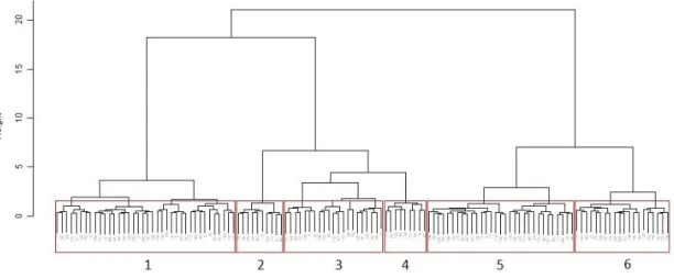
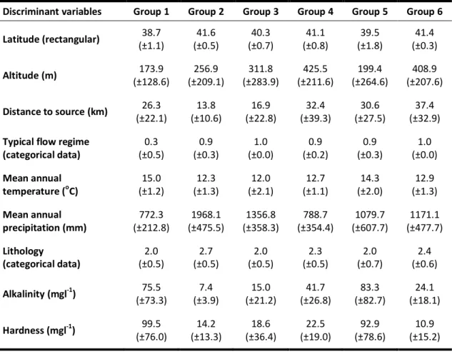
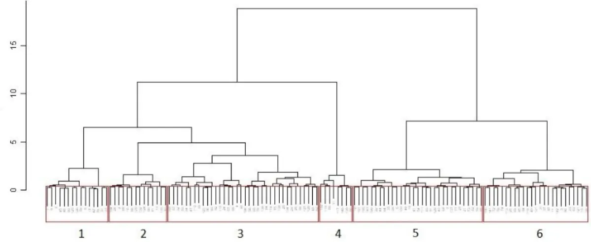
Figure 30 - Cluster of calibration reference sites used for RIV DIAT model construction. Each number corresponds to a group. ... 45
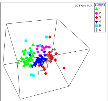
Figure 31 - Three-dimensional MDS ordination of six groups based on diatom references from the calibration dataset of RIV DIAT model. ... 46
Figure 32 - RMSE (O/E) values for both calibration (c) and validation (v) datasets are shown as well as the corresponding maximum of RMSE for calibration dataset (black line) and the selected model (red circles). ... 49
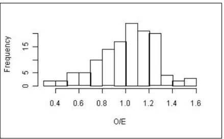
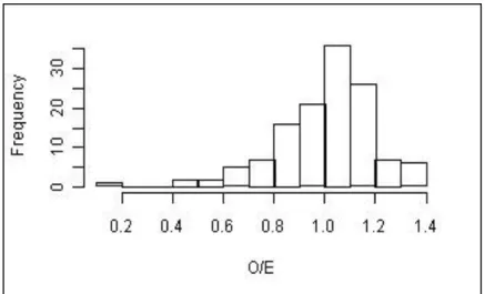
Figure 33 - Distribition of frequencies of the O/E50 of all reference sites in the RIV DIAT model. ... 50
Figure 34 - Three-dimensional MDS ordination of the 6 groups based on macroinvertebrate reference community from the calibration dataset of RIV INV model. ... 51
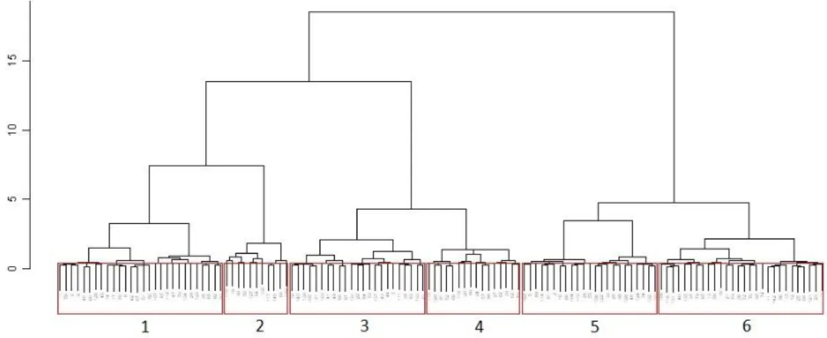
Figure 35 - Cluster of calibration reference sites used for RIV INV model construction. Each number corresponds to a group. ... 51
Figure 36 - RMSE (O/E) values for both calibration (c) and validation (v) datasets are shown as well as the corresçponding maximum of RMSE for calibration dataset (black line) and the selected model (red circles). ... 54 Figure 37 - Distribution of frequencies of the O/E 50 of all reference sites used in the RIV INV model. ... 55 Figure 38 - Cluster of calibration reference sites used for RIV INV+DIAT model construction. Each number corresponds to a group. ... 56 Figure 39 - Three-dimensional MDS ordination of the 6 groups based on the combined biological reference community of macroinvertebrates and diatoms from the calibration dataset of RIV INV+DIAT model. ... 56 Figure 40 - RMSE (O/E) values for both calibration (c) and validation (v) datasets are shown as well as the corresçponding maximum of RMSE for calibration dataset (black line) and the selected model (red circles). ... 60 Figure 41 - Distribution of frequencies of the O/E 50 of all reference sites used in the RIV INV+DIAT model. ... 60 Figure 42 - Cluster of the calibration reference sites used for BEAST DIAT model construction. Each number corresponds to a group. ... 63 Figure 43 - Three-dimensional MDS ordination of the six groups based on diatom reference community from the calibration dataset of BEAST DIAT model. ... 63 Figure 44 - Cluster of the calibration reference sites used for BEAST INV model construction. Each number corresponds to a group. ... 66 Figure 45 - Three-dimensional MDS ordination of the six groups based on biological reference community from the calibration dataset of BEAST INV model. ... 67 Figure 46 - Cluster of the calibration reference sites used for BEAST INV+DIAT model construction. Each number corresponds to a group. ... 71 Figure 47 - Three-dimensional MDS ordination of the six groups based on biological reference community from the calibration dataset of BEAST INV+DIAT model. ... 72 Figure 48 - Box plots representing the examples of clear relationship between increasing pressure level (for total phosphorous, HQA, dissolved O2 and nitrates variables) and the
classification attributed by RIV INV model. ... 87 Figure 49 - Box plots representing the examples of clear relationship between increasing pressure level (for ammonia, BOD5, nitrites and pH variables) and the classification
attributed by RIV DIAT model... 88 Figure 50 - Box plots representing the examples of clear relationship between increasing pressure level (for HMS, HQA, dissolved O2 and nitrites variables) and the classification
attributed by RIV INV+DIAT model. ... 88 Figure 51 - Box plots representing the examples of clear relationship between increasing pressure level (for riparian zone, total phosphorous, dissolved O2 and nitrites variables) and
the classification attributed by BEAST DIAT model. ... 89 Figure 52 - Box plots representing the examples of clear relationship between increasing pressure level (for HQA, HMS, ammonia and nitrates variables) and the classification attributed by BEAST INV model. ... 89 Figure 53 - Box plots representing the examples of clear relationship between increasing pressure level (for total phosphorous, morphological condition, HMS and nitrates variables) and the classification attributed by BEAST INV+DIAT model. ... 90 Figure 54 - Principal Component Analysis of all sites based on disturbance variables ... 91
Index of Tables
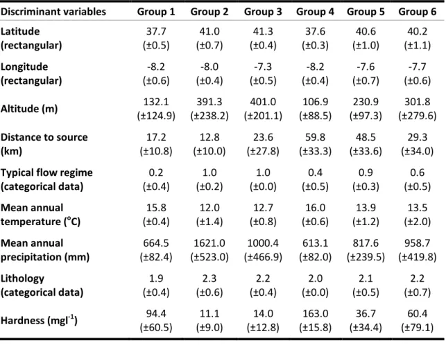
Table 1 - Potential discriminant variables used to characterize the reference sites and build predictive models. ... 38 Table 2 - Environmental variables measured or calculated for each test site. In italic are those not used as pressure variables... 39 Table 3 - Most representative taxa of the 6 reference groups of RIV DIAT model, obtained by SIMPER analysis. The diatoms represented were found in 50% or more of the sites. ... 47 Table 4 - Environmental characterization of the 6 reference groups of streams used in the RIV DIAT predictive model. ... 48 Table 5 - RIV DIAT model validation with 14 reference sites not included in the model construction. ... 50 Table 6 - Most representative taxa of the 6 reference groups of RIV INV model, obtained by SIMPER analysis. The invertebrates represented were found in 50% or more of the test sites... 52 Table 7 - Environmental characterization of the 6 reference groups of streams used in the RIV INV predictive model. ... 53 Table 8 - RIV INV model validation with 14 reference sites not included in the model construction. ... 55 Table 9 - Most representative taxa of the 6 groups of RIV INV+DIAT model, obtained by SIMPER analysis. The invertebrates and diatoms represented were found in 50% or more of the sites. ... 58 Table 10 - Environmental characterization of the 6 reference groups of streams used in the RIV INV+DIAT predictive model. ... 59 Table 11 - RIV INV+DIAT model validation with 14 reference sites not included in the model construction. ... 61 Table 12 - Summary of the characteristics of the three RIVPACS predictive models. ... 62 Table 13 - Most representative diatom taxa of the 6 reference groups of BEAST DIAT model, obtained by SIMPER analysis. The diatoms represented were found in 50% or more of the sites. ... 64 Table 14 - Environmental characterization of the 6 reference groups of streams used in the BEAST DIAT predictive model. ... 65 Table 15 - BEAST DIAT model validation with 14 reference sites not included in the model construction. ... 66 Table 16 - Most representative taxa of the 6 reference groups of BEAST INV model, obtained by SIMPER analysis. The invertebrates represented were found in 50% or more of the sites. ... 68 Table 17 - Environmental characterization of the 6 reference groups of streams used in the BEAST INV predictive model. ... 69 Table 18 - BEAST INV model validation with 14 reference sites not included in the model construction. ... 70 Table 19 - Most representative taxa of the 6 reference groups of BEAST INV+DIAT model, obtained by SIMPER analysis. The invertebrates and diatoms represented were found in 50% or more of the sites. ... 73 Table 20 - Environmental characterization of the 6 reference groups of streams used in the BEAST INV+DIAT predictive model. ... 74 Table 21 - BEAST INV+DIAT model validation with 14 reference sites not included in the model construction. ... 75
Table 22 - Summary of the characteristics of the three BEAST predictive models. ... 75 Table 23 – Water quality classes attributed to test sites by the three predictive models, RIV DIAT, RIV INV and RIV INV+DIAT... 76 Table 24 - Classes attributed to test sites by the three predictive models, BEAST DIAT, BEAST INV and BEAST INV+DIAT... 77 Table 25 – Classification of test sites according to what is used in the context of the WFD (worst classification obtained by the individual diatom or the macroinvertebrate RIVPACS models) and RIV INV+DIAT model. ... 78 Table 26 - Classification of test sites according to what is used in the context of the WFD (worst classification obtained by the individual diatom or the macroinvertebrate BEAST models) and BEAST INV+DIAT model. ... 79 Table 27 - Spearman rank correlation (rs) and respective P value between quality classes of the three RIVPACS type of predictive models and pressure variables for reference and test sites... 81 Table 28 - Spearman rank correlation (rs) and respective P value between quality classes of the three BEAST type of predictive models and pressure variables for reference and test sites... 82 Table 29 - Spearman rank correlation (rs) and respective P value between quality classes of the RIV INV+DIAT and WFD and pressure variables for reference and test sites. In bold the highest significant correlations between methods, for each variable are highlighted. ... 84 Table 30 - Spearman rank correlation (rs) and respective P value between quality classes of the BEAST INV+DIAT and WFD and pressure variables for reference and test sites. In bold the highest significant correlations between methods, for each variable are highlighted. ... 85 Table 31 – Spearman rank correlation (rs) and respective P value between classes of all the approaches and pressure variables for reference and test sites. The red rectangles show the highest and the grey ones the second highest significant correlations between methods, for each variable. ... 86 Table 32 - Spearman rank correlation (rs) and respective P value between quality classes of the three RIVPACS and BEAST predictive models and SCORE 1 of PCA analysis. The red rectangles signed the highest and the gray ones the second highest significant correlations between methods. ... 92
Acronym list
ANOVA Analysis of Variance ASPT Average Score Per Taxon
BEAST Benthic Assessment of Sediment BMWP Biological Monitoring Working Party
CEE Índice da Comunidade Económica Europeia DA Discriminant Analysis
DFA Discriminant Function Analysis DGA Atlas Digital do Ambiente
E Expected
EQR Ecological Quality Ratio GQA General Quality Assessment HMS Habitat Modification Score HQA Habitat Quality Assessment IBD Indice Biologique Diatomées IBI Index of Biotic Integrity
IBMWP Iberian Biological Monitoring Working Party INAG Instituto Nacional da Água
IPS Indice de Polluossensibilité Spécifique IPtI Invertebrate Portuguese Index
MDS Non-metric Multidimensional Scaling
MN Mean Value
NRA National River Authority
O Observed
O/E Observed Expected ratio PC Probability of Capture
PCA Principal Component Analysis
RIVPACS River Invertebrate Prediction And Classification System RMSE Root Mean Squared Error
RSSD Replicate Sampling Standard Deviation SD Standard Deviation
SI Saprobien Index TDI Trophic Diatom Index
UK United Kingdom
UPGMA Unweight Pair Group Method with Arithmetic mean USA United States of America
Chapter 1 - INTRODUCTION
Water degradation is a result of human activities, as most societies are clustered as close as possible to rivers, facilitating waste disposal (Perry and Vanderklein 1996). The realization that unmanaged ecosystems will soon fail to provide free ecological services, such as drinking water, fish and waste assimilation, has led to a considerably improvement in the water legislation viewing the protection of the aquatic ecosystems (Cairns Jr. and Pratt 1993).
Until the 90s, most water quality monitoring programs were focused only on chemical analysis. This is an accurate approach but presents the disadvantage of providing a fragmented overview of ecosystem health, as well as providing information of the water quality only at the time of sampling (Alba-Tercedor and Sánchez-Ortega 1988, Atazadeh et al. 2007, Bere and Tundisi 2011a). On the other hand, assessment based on biological communities has several advantages over the physical and chemical measurements of water quality: they show the cumulative effects of present and past condition and therefore provide a direct, holistic and integrated assessment of environmental conditions that are highly variable in space and time (Bere and Tundisi 2011a, Stoermer and Smol 1999). Furthermore, the use of biological indicators for assessment of water quality is now mandatory under the European Water Framework Directive of 2000 which should achieve the good ecological status (quantitative and qualitative) until 2015 and ensure the sustainable use of aquatic environments (WFD; EC Parliament and Council 2000).
Biomonitoring is defined as the measurement and evaluation of the ecosystem condition using biological responses to impacts, usually caused by human activities but also implies quality control through corrective and preventive actions when the expected conditions are not achieved (Matthwes et al. 1982). The idea of biological monitoring is not new. In the early days of the industrial revolution, canaries were kept in underground coal mines and if they showed adverse responses to conditions, the miners abandoned the mine (Cairns Jr. and Pratt 1993). The modern history of aquatic biomonitoring began in Europe in the twentieth century. Studies of biological indicators relied on the
identification of indicative species of human degradation and biological classification of streams (Cairns Jr. and Pratt 1993). The use of biological communities (fishes, invertebrates, macrophytes and algae) as indicators of water quality is evolving and are becoming more widely used while initially mainly invertebrates were used. Especially in the past two decades, several methods have been developed to assess streams ecological health such as autoecological indices, indices of biotic integrity, predictive models and others.
1.1 Macroinvertebrates as bio-indicators of water quality
The term macroinvertebrate describes the animals that have no backbone and that can be seen by the naked eye. Normally these organisms exceed 500 µm of body size. They are mostly insects but also decapods, crustaceans, mollusks, leeches, oligochaetes and planarians. The majority of freshwater insects has an amphibiotic life cycle and spends their adult stage on land. Macroinvertebrates commonly inhabit the bottom substrates (sediments, debris, logs, macrophytes, filamentous algae, etc.) and are referred as benthic macroinvertebrates or macrobenthos (Cummins 1992, Rosenberg and Resh 1993).
The macroinvertebrate communities are the most widely used for assessing water quality for several reasons. They are found along the river continuum, are cosmopolitan and respond to changes in water quality resulting from anthropogenic disturbances (Azrina et al. 2006). Because of their limited migration, they are good indicators of localized impacts. These organisms have a complex life cycle of approximately 1 year so they can integrate and reflect the environmental changes that they have gone through (Barbosa et al. 2001). The freshwater macroinvertebrates include representatives of many insect orders that contribute to important ecological functions such as decomposition, nutrient cycling and play an important role in food webs as both consumers and prey (Kenney et al. 2009). They are relatively easy to identify to family level and many taxa can be identified to lower taxonomic levels. There are many species within a community with different ranges of tolerance and sensitiveness to stress that provides information for interpreting the cumulative effects (Abbasi and Abbasi 2011). Sampling of macroinvertebrates in wadeable rivers is relatively easy and inexpensive and
has minimal adverse effect on the resident biota (Barbour et al. 1999). In addition, methods for analyzing their data are well established.
Many methods based on macroinvertebrates for evaluating ecosystems health have been developed through time and implemented in Europe in the beginning of the XXth century. Most of them are based on Kolkwitz and Marsson (1908, 1909) and originated new biotic indices (Figueroa et al. 2003).
Biotic indices are numerical expressions combining a quantitative measure of species diversity with the qualitative information on the ecological sensitivity of individual taxa (Bieger et al. 2010). They are based on the assumptions that the number of taxonomic groups decreases and that macroinvertebrates follow this disappearing sequence with the increase of organic pollution: Plecoptera, Ephemeroptera, Trichoptera, Gammarus,
Asellus, red migdes Chironomidae and Tubificidae. The declining order only reflects their
tolerance to organic pollution (Czerniawska-Kusza 2005).
Beck was the person who popularized the term “biotic index”. Beck’s Biotic Index (Beck’s BI - 1954) is based on macroinvertebrates tolerances to organic pollution and was developed in Florida. It’s considered the real first biotic index because it included description of field procedures and identification to the species level. Organisms were divided into three classes: “Class I” for the intolerant and “Class II” for the facultative and “Class III” for those tolerant to organic pollution. However, he decided not use the tolerant organisms because they could be found in clean waters, but in lower abundance. The Beck’s indice value can oscillate between 0 and 40, but it not takes into account the organism’s abundance, only attributes the numeric values of 2 and 1 to the “Class I” and “Class II”, respectively. So, final score of the index for a site is calculated by summing the number of species of “Class I” multiplied by two, with the number of species of “Class II” (Davis 1995).
The Trent Biotic Index [TBI – (Woodiwiss 1964)] was developed by the Trent River Authority in England. The sampling included all available habitats during 10 minutes with a hand-net. The index’s value is based on the presence or absence of six “groups” of invertebrates with different degrees of tolerance to organic pollution. The final value can
vary from 0 (grossly polluted) to 10 (unpolluted). The Trent Biotic Index served as model to other several biotic indices (Muralidharan et al. 2010).
The Belgian Biotic Index [BBI – (De Paw and Vanhooren 1983)] was developed in Belgium and combined different biotic indices. All available habitats are sampled with a 300-500 µm mesh hand-net during 3 or 5 minutes, depending on the width of the river. The macroinvertebrates are preserved in situ and identified to family or genus levels in the laboratory. The final value varies from 0 (very heavily polluted) to 10 (unpolluted) (Abbasi and Abbasi 2011).
The Biological Monitoring Working Party (BMWP) Score index (Chesters 1980) was developed in Britain and has been widely applied. The macroinvertebrates are identified to family level and each one receives a score between 1 (most tolerant) and 10 (least tolerant). This index does not take into account the abundance. The BMWP score is the sum of individual scores that can be divided by the number of taxa with score to produce the Average Score Per Taxon (ASPT). The ASPT is less influenced by season and sample size than BMWP score (Muralidharan et al. 2010).The Iberian IBMWP – (Alba-Tercedor et al. 2002) is and adaptation of the BMWP Score System to Iberian rivers. All available habitats are sampled over a 100m stretch with a kick-net with 250 µm mesh size and the invertebrates are identified to family level. The final IBMWP score, number of taxa and IASPT (IBMWP score divided by number of taxa) are calculated for a site based on all the taxa collected and observed (Abbasi and Abbasi 2011). These indices were, until the implementation of the WFD, the most commonly used in Portugal and Spain.
Nowadays, the official index in Portugal is the IPtI (Invertebrate Portuguese Index), established by INAG (2009). This is a multimetric index produced during the Intercalibration Exercise carried out by the Mediterranean Geographical Intercalibration Group (Med-GIG), in which Portugal took part and which aimed the comparability of quality assessments and compliance with the WFD. The index is divided in two indices, the IPtIN, applied to rivers in North of Portugal and the IPtIS, applied to rivers in the South
and Littoral. It’s calculated as the weighted sum of some metrics, each normalized using the ratio between the obtained values and the corresponding reference values which is
dependent on the river type. The final value (Ecological Quality Ratio-EQR) varies between 0 and approximately 1 (for reference sites).
Currently, over the world, the most common methods for assessing water quality are the multimetric indices and the multivariate approaches. The multimetric indices integrate into a single value different metrics (e.g. taxonomic diversity, exposure of the community to stressors) of the biological community that are sensitive to a broad range of human activities. The chosen metrics are calculated from the taxa data matrix at the sites and can be combined (hence “multimetric”) to enhance predictability compared to individual ones (Milner and Oswood 2000). The first multimetric index was developed by Karr (1981) in the USA, the IBI (Index of Biotic Integrity). This index incorporated zoogeographic, ecosystem, community and populations aspects of fish assemblages into a unique ecologically-based index.
The multivariate approaches rely on multivariate statistical methods to uncover patterns in taxonomic composition and will be described in detail later in this chapter.
In spite of the macroinvertebrates being the preferred organisms for assessing water quality (Harding et al. 2005), they also present some disadvantages such as their aggregated distribution which implies many subsamples to collect a representative sample. Moreover, some insects are absent in the water during part of the year and this should be taken into account in the interpretation of the results (Muralidharan et al. 2010). According to Charles (1996), the use of algae for monitoring rivers has increased because of these limitations with benthic invertebrate methods, coupled with significant improvements in technologies for algal assessment. The algal class Bacillariophyceae, the diatoms, is one of the groups of organisms that fulfill the requisites needed for biological monitoring.
1.2 Diatoms as bio-indicators of water quality
The word “diatom” comes from Greek, which means cut in two. The characteristic feature of diatoms is its rigid cell wall composed of silica, called frustule. Each frustule is box-like in structure and made of two parts, the valves. Diatoms are eukaryotic microscopic unicellular organisms, although chains of cells and colonial aggregations may also occur. These algae are pigmented and most are photosynthetic. Diatoms are
ubiquitous in their distribution and can be found in all waters except the hottest and most hyper saline. In freshwater, diatoms can live in open water (planktonic) or attached to substrata (periphytic). Periphytic diatoms are found attached to rocks (epilithon), sand grains (epipsammon), plants (epiphyton) and soft sediments (epipelon) (Bold and Wynne 1985, Jones 2007).
Within the algae, diatoms have been the main focus of bioassessment studies (Bold and Wynne 1985, Jones 2007, Lee 1980, Bellinger et al. 2006). These organisms play a crucial role as primary producers in streams and due to their position in food webs it is expected that any disturbance in diatom populations affect the whole aquatic community (Andrén and Jarlman 2008). Diatom assemblages are considered useful tools in water quality monitoring for many other reasons. They form a large part of the benthos (about 90%), are ubiquitous and occur in all types of aquatic systems (Solak and Acs 2011). Due to their short generation time (high reproduction rate), diatoms show quick responses to water quality degradation by changing species composition and diversity (Bere and Tundisi 2011a). For a large number of species ecological information is available and many show narrow ranges of tolerance to several abiotic features. This information in conjunction with the persistence of frustules in sediments has been used for historical reconstruction (Cooper 1995). These organisms can be preserved and stored indefinitely as permanent slides and reinvestigated whenever necessary (Solak and Acs 2011). In addition, diatoms are easy to sample and their identification is possible through taxonomic guides because it is mainly based on frustule morphology (Aboal et al. 2003, Krammer 2000, 2002, 2003, Krammer and Lange-Bertalot 1986, 1988, 1991a, 1991b, Lange-Bertalot 2001, Lange-Bertalot et al. 2003, Levkov 2009, Werum and Lange-Bertalot 2004). Nevertheless, the use of these organisms presents the disadvantage of requiring taxonomic expertise (Solak and Acs 2011).
The assessment of water quality in freshwater habitats with benthic diatoms has a long history and the first studies date back a century ago (Kireta et al. 2012). These methods have been reviewed by many authors (Lowe and Pan 1996, Patrick 1973, Rosen 1995, Stevenson and Lowe 1986, Whitton and Kelly 1995, Whitton et al. 1991). Within the last
decades diatom-based indices became popular worldwide, especially in Europe (Bere and Tundisi 2011a).
According to Stevenson and Pan (1999), two different approaches using diatoms have been developed: the autoecological indices based on Kolkwitz and Marsson (1908, 1909) works (Butcher 1947, Descy 1979, Slàdecek 1973, Zelinka and Marvan 1961) and the studies centred on the diversity of diatoms as an indicator of river health based on Patrick’s monitoring studies (Patrick 1949, Patrick and Strawbridge 1963, Patrick et al. 1954). The autoecological indices use the relative abundance of species and are based on the assumption that species have specific optima and tolerances, sensitivities or preferences for environmental conditions (Stevenson 1998). Diatoms are known to respond to eutrophication, organic pollution, heavy metals, salinity, pH, pesticides, and their sensitivity/tolerance to those environmental characteristics differ among species (Stevenson and Pan 1999). Most of those indices are based on the weight average equation of Zelinka and Marvan (1961)and, according to Rimet et al. (2005), there are as many indices as the number of researchers working in the field. The most significant development during the 80’s was the Indice de Polluossensibilité Spécifique (IPS – Cemagref 1982) that provides integrated assessment of a range of water quality variables such as organic pollution, eutrophication, salinity and toxic substances (Solak and Acs 2011). More indices were developed in other countries, like the Trophic Diatom Index (TDI) in UK (Kelly and Whitton 1995), the Saprobienindex (SI) in Austria (Rott et al. 1997) and the Indice Biologique Diatomées (IBD) in France (Lenoir and Coste 1996).
Some characteristics of diatom communities have also been used to assess the ecological integrity of streams such as biomasss, morphology, chemical ratios (chl a, N, P, heavy metals, etc), growth, dispersal and metabolic rates. Usually these features are used together with the characteristics of the entire periphyton or plankton assemblages (Stevenson and Pan 1999).
In Portugal, under WFD legislation, two different diatom-based indices were adopted, the IPS for the North of Portugal and the European Index (CEE – Descy and Coste 1990) for the South of Portugal. The IPS index is based on Descy’s method and differs only on the indicator and sensitivity values of taxa. The species were grouped in 5 classes from 1
(tolerant species) to 5 (sensitive species). The final values of IPS are then converted into EQRs by dividing them by the reference value for their river type (as established in the WFD implementation). Finally intervals of these values correspond to quality classes (high = 1, good = 2, moderate = 3, poor = 4 and bad = 5) (INAG, I. P. 2009). The CEE index is based on a two-way entry table, which includes 208 taxa. In this table, taxa are grouped into 8 groups arranged in descending order of sensitivity to pollution (group 1 more sensitive and group 8 more tolerant). Vertically, there are 4 subgroups of taxa (9 to 12) with restricted geographic distribution based on alkalinity and mineralization. The index value is obtained by crossing the median values of the group and subgroup (those containing 50% or more of abundance of the taxa involved in the calculation), which is then normalized and can vary from 1 (strongly polluted) to 20 (unpolluted) (INAG, I. P. 2009).
Biotic indices are useful tools for rapid bioassessments but they should be wisely interpreted because of their limitations. The most important is the restricted applicability due the geographic area that they are built for (Abbasi and Abbasi 2011). There are evidences that indices developed for one area are less successful when applied in others because of the floristic differences among regions (Bere and Tundisi 2011a). According to Besse-Lototskaya et al. (2011), European indices use different ecological profiles for the same species because most of them are rare and difficult to define, and therefore, not robust.
1.3 Predictive Models overview
More recently, predictive models appeared as an alternative to the traditional indices in some regions of the world. The predictive models are based on multivariate analysis and follow the concept of Reference Condition. Reynoldson et al. (1997) defined the reference condition as a group of sites in which physical, chemical and biological features are within the range characterized as undisturbed or minimally disturbed. The predictive models measure river health as the alteration of the biological community composition to an expected community under reference conditions. Predictive models are founded on the biological classification of reference sites, based on the similarity between species composition (Reynoldson et al. 1997). According to Zamora-Muñoz and Alba-Tercedor
(1996), the main advantage of multivariate methods is the small reduction of multidimensional data with consequent minimal loss of information, identifying the direction of data variability. The greater disadvantage is the huge effort in the initial construction phase. Nevertheless, this problem can be bypassed with software that integrates model analysis and yields easily understandable results (Feio 2004).
Initially, the predictive models were based on macroinvertebrate communities. The first one, RIVPACS (River InVertebrate Prediction And Classification System – Wright et al. 1993) was developed in Great Britain. It was followed by the BEAST (BEnthic Assessment of Sediment – Reynoldson et al. 1995, 1997) developed in Canada and the AUSRIVAS in Australia (AUstralian RIver Assessment Scheme – Marchant et al. 1997, Simpson and Norris 2000). Later, other predictive models appeared based on fishes (Kennard et al. 2006), diatoms (Chessman et al. 1999, Feio et al. 2007) and macrophytes (Aguiar et al. 2011).
In Portugal, the first predictive models were built initially for the Mondego River basin based on macroinvertebrate communities and following the BEAST approach (Feio et al. 2004, 2006a, 2006b, 2007). Three predictive models were built with 55 reference sites using three levels of taxonomic resolution: 1) the lowest practical taxonomic level (Feio et al. 2007); 2) family level (Feio et al. 2006b) and 3) order level (Feio et al. 2006a). Models performances were tested with 20 test sites that covered a wide range of stream types and all seasons. The best performing model was the one built at the lowest practical taxonomic level.
Since then, other studies addressing predictive models based on different approaches, using different biological communities have been developed (review in Feio & Poquet 2011). Feio et al. (2010) built also predictive models based on functional parameters: one for decomposition (D model), using microbial and total decomposition rates in oak and alder leaves and the other based on biofilm characteristics (B model), using sediment respiration rates, biofilm growth and total chlorophyll a of biofilm on natural substrata, the autotrophic index and fungal biomass on conditioned oak leaves. This study showed that functional variables, especially decomposition, can be useful ecological indicators in monitoring programs. Aguiar et al. (2011) built two macrophyte predictive models, one
based on RIVPACS and the other based on BEAST approaches. The models were developed for the entire country (Portugal) and the objectives were to test the suitability of two predictive modeling approaches to macrophyte communities as a water-quality assessment tool and compare their performance with other more common approaches. Almeida and Feio (2012) tested the adaptation of the RIVPACS/AUSRIVAS methods to Portuguese rivers through the development of a predictive model based on diatoms (DIATMOD model). Mendes et al. (2012) used two diatom predictive models developed for Portugal: the MoDi based on BEAST and the DIATMOD based on RIVPACS/AUSRIVAS approaches. The goals of this study were to determine the effect of substrate type and the evaluation method on the assessment of water quality.
The RIVPACS, BEAST and AUSRIVAS approaches are within the most commonly used predictive models (Feio and Poquet, 2011). However, the RIVPACS is probably the furthermost popular approach and is now well established in several countries such as U.K., Australia, Canada, Sweden and the Czech Republic (Clarke and Murphy 2006).
1.3.1 RIVPACS approach
The development of the RIVPACS models started in October 1977 with two major goals: 1) development of a biological classification of minimally polluted waters in Great Britain based on macroinvertebrate communities; 2) determine if those communities could be predicted based on physical and chemical features for each site.
In 1986, the first version of RIVPACS was implemented on a microcomputer and made available to water industry biologists throughout Great Britain for testing. By then, RIVPACS I included 370 reference sites which resulted in 30 groups. The classification and predictions were based on species level (Wright 2000). In 1990, the National River Authority (NRA) funded the development of an operational version, the RIVPACS II, for use in the 1990 River Quality Survey. RIVPACS II was used at almost 9000 sites in 1990 River Quality Survey throughout England, Wales and Scotland and on a more experimental basis in Northern Ireland where there were no local references. In this version, further streams were added to give a total of 438 reference sites which resulted in a new classification with 25 groups, as well as other improvements (Wright 2000). The 1995 General Quality Assessment (GQA) required an upgrade of the system, so data
collected from sites with high biological quality, sites recommended by local biologists and sites of Northern Ireland were added to develop RIVPACS III. One important modification was also implemented: while RIVPACS II was based on qualitative species data, RIVPACS III used qualitative species data plus family data to characterize each site (Wright 2000). Several other improvements were made to the successive versions of RIVPACS such as standardizing sampling protocols, assessing different taxonomic levels, developing single and combined season models, predictive models using both qualitative and quantitative data, studying alternative procedures for site classification and prediction, assessing the uncertainty of the predictive systems outputs (Feio and Poquet 2011). The RIVPACS III+ represents the major step forward through the incorporation of error terms for the O/E ratios used to assess site quality and provides a mechanism for detecting statistically significant spatial and temporal differences between the macroinvertebrate assemblages of sites (Wright 2000). It is implemented in a software package and it was used under the Water Framework Directive in U.K. (Feio and Poquet 2011).
A RIVPACS predictive model is built in several steps. The first and crucial step is the selection of reference sites (Clarke et al. 2003). The next step is collecting the biological and environmental data. Only environmental features not affected by stressors can be used as predictors. Then, the reference sites are grouped according to their similarity between species composition and by means of ordinations obtained from the correspondence analysis method. Then a Discriminant Function Analysis (DFA), which predicts group membership based on multiple linear regressions, is used to select the potential environmental descriptors that best discriminate the reference groups. To determine the discriminatory power of the DFA, the RIVPACS relied on re-substitution and cross-validation analyses. These analyses provide a percentage value of reference sites correctly located in their original groups. In the cross-validation analysis, one reference site is left aside from the others each time and later it is used to rebuild the DFA model. Then the reference sites are used as test sites and the number of sites attributed to its original group gives the percentage of correct classification. The re-substitution analysis occurs the same way as cross-validation, but the DFA model is not
rebuilt for each site. The probability of a new test site belonging to a group can be calculated from the Mahalanobis distance between test site and center of each biological group (Clarke et al. 2003). RIVPACS uses these probabilities of belonging to each reference group to calculate the expected fauna. The final probability of capture (Pc) for a taxon in a test site is calculated as the sum of the probabilities of belonging to each biological reference group, weighted by the frequency of occurrence of that taxon inside each group (Feio and Poquet 2011). The deviation of the observed (O) from the expected taxa (E) is measured by the ratio O/E. Low ratio values (O/E close to 0) means that test sites are strongly impacted by some environmental stressor while ratio values close to 1 means that a site is near to reference (Hawkins et al. 2000).The expected number of taxa (E) is calculated as the sum of individual Pc for all taxa found in a test site. Only taxa with Pc ≥ 0.5 are usually used to calculate E because rare taxa appear to decrease the performance of models. The standard deviation (SD) of O/E characterizes the magnitude of predictor error and low SDs indicates that the model accounts for much of natural variability and provides good predictions. The final biological evaluation obtained by the RIVPACS approach can vary along an assessment gradient (O/E gradient). Based on the taxa predicted to occur, the RIVPACS approach also produces two biotic indices: the ASPT and BMWP for each test site. For the ASPT the lower 5%, and for the number of taxa and the BMWP the lower 10% of the reference O/E distribution are then used as a threshold to considerer the test sites as impacted by setting the quality classes (below reference) in order to calculate the deviation of a site from the reference condition (Feio and Poquet 2011).
1.3.2 BEAST approach
The BEAST approach was developed in Canada to create criteria for sediment quality of the North American Great Lakes by Reynoldson et al. (1995, 1997). This approach was based on methods developed in the United Kingdom with the main goal to determine predictive associations between the macroinvertebrates and the physic-chemical parameters. During the period from 1991 to 1993, 345 samples were collected from 245 sites and included in the construction of the predictive model (Reynoldson et al. 1995). Later, Rosenberg et al. (2000) also built a BEAST model type based on macroinvertebrates
collected from 127 reference sites during autumns of 1994 and 1995. This model was developed for the Fraser River located in North America.
The BEAST models are built in 3 steps: 1) first a PCA (Principal Component Analysis) analysis was used to identify patterns in environmental data through the ordination axes developed from the biological data; 2) determine the environmental variables that best discriminate the biological groups using a DA (Discriminat Analysis); and 3) identify the environmental variables that differ significantly between the biological groups through an ANOVA (Analysis of Variance) (Feio and Poquet 2011).
The major difference between RIVPACS and BEAST approaches (Figure 1) is the assessment of test sites. In BEAST models, the community composition of the test site is compared to the sites included in the biological reference group to which the test site is most likely to belong, based on their environmental characteristics (discriminant predictors). These data are merged in the same matrix, re-ordinated in a MDS-ordination space and plotted, in the original method, in a banding system defined by Gaussian probability ellipses (90, 99, 99.9%). The distance of the test site from the ordination centroid results in the biological assessment. A site located in the first band (inner ellipse) is considered equivalent to the reference, a site located in the second band (90-99%) was potentially different from reference, a site located in the third band (99-99.9%) is different from reference and a site located in the fourth band (beyond 99.9%) is very different from the reference. Thus, the BEAST predictive model gives a direct evaluation of the water status (Reynoldson et al. 1997, Feio and Poquet 2011).
1.4 Goals
Independently of the biological assessment methods used, when more than two biological elements are evaluated, there is a need for a global assessment of the studied site. Presently, that is commonly done in Europe by combining the assessments a
posteriori. This combination is done based on the “one-out all-out” approach, which is a
conservative approach that many researchers consider unrealistic.
Figure 1 - Flowchart of assessment methods using BEAST and RIVPACS approaches. Adapted from
Therefore, the main goal of this study is to evaluate if a predictive model based on the evaluation of biodiversity using the taxa from two biological elements (macroinvertebrates and diatoms), produces a simpler and simultaneously more holistic and accurate assessment of streams health than individual assessments combined a
posteriori. For that purpose, we used two different approaches due to their different
characteristics: 1) the RIVPACS technique which is based on presence/absence data and only includes frequent taxa and 2) the BEAST methodology, based on abundance data that takes into account the entire community. For comparison, we built six predictive models, three of them based on RIVPACS approach and the other three based on BEAST approach, for continental Portugal: two for diatoms, another two for macroinvertebrates, and the last two integrating diatom and invertebrate assemblages. For all the six predictive models, 23 impacted stream sites affected by mine drainage, organic contamination and industrial effluents were used as test sites. The performance of the combined models was achieved by comparing the assessment of the test sites against the assessments made by the individual ones. Those assessments were also compared with those that would be obtained with the “one-out, all out” approach currently used in Europe.
Chapter 2 – STUDY AREA
The study area (Figure 2) comprises three adjacent river catchments with a total area of 11215 km2 located in central Portugal: Mondego, Vouga and Lis. This region has a temperate Atlantic climate and highly diverse geological landscapes (Feio et al. 2009a).
Figure 2 - Hydrological basins of Portugal. The study area is marked with a black outline.
The Mondego is the largest river entirely in national territory located between 39o46’ and 40o48’ N and 7o14 and 8o52’ W, covering an area of 6670 km2. The river starts to flow in Serra da Estrela at 1547 m of altitude in a small fountain called “Mondeguinho” and runs along 300 km until it reaches the Atlantic Ocean, nearby the city of Figueira da Foz. The main tributaries of this river are Dão on the right bank and Pranto, Arunca, Ceira and Alva rivers on the left one. The basin has an approximately rectangular shape elongated in NE-SW direction. Along the river, three distinct segments can be distinguished: high, medium and low sections. In the high section the river flows through glacial valleys in which the substrate is coarse and mostly granite and schist. In the medium section the river flows in valleys between Serra da Estrela and Coimbra where the Dão, Alva and Ceira rivers converge. The dominant substrates remain the same as in the high section, granite and schist. In the low section the river runs through Coimbra in open valleys to floodplains and the bedrock is limestone with fine sediments (Feio et al. 2007, PBH 1999a). The main anthropogenic pressures felt in the littoral (low section) are agriculture (extensive rice fields) and urban effluents. In the interior the main impacts are the presence of dams and weirs, some milk and cheese industries and mine drainage (Feio et al. 2009a, Feio et al. 2010).
The Vouga river source is located at 930 m of altitude in Serra da Lapa (Chafariz of Lapa), located in Viseu district. The Vouga’s basin is the second largest that runs entirely in Portugal and it is limited at 40o15’ and 40o5’ N and 7o33’ and 8o48’ W. The Vouga river covers a total area of 3706 km2. This basin is composed by a hydrographic set of rivers that discharge very close to the Vouga’s mouth in Aveiro estuary (Ria) that communicates with the ocean. The main rivers of this set are Águeda, Cértima, Caster, Antuã and Boco rivers and also Corujeira stream in which the substrate is schist and granite. The Vouga river flows along different types of valleys: through an upland until São Pedro do Sul where the basin is elongated-shaped, in a valley with a high slope between São Pedro do Sul and Albergaria-a-Velha, through open valleys until Aveiro and in the estuary (PBH 1999b). The major impacts affecting this basin are the large-scale eucalyptus plantations and paper pulp industries (Feio et al. 2010).
The Lis river is the smallest catchment covering an area of 945 km2 and it is limited between 39o30’ and 40o00’ N and 8o35’ and 8o00’ W. Lis basin topography is smooth, mostly below 200 m of altitude. The maximum altitude is 562 m in Pedra of Altar. The main water courses are Lis and Lena rivers that run through a limestone massif and an old pine forest. The valleys of Lis and Lena rivers are wide and flat, typical of alluvial floodplains. The Lis valley only narrows when it crosses the anticlinal structure of Leiria and then extends downstream of the confluence of Lena where it forms an alluvial floodplain with 1 km wide. The coastline consists of dunes that include some of the highest in our country (50 m) (Feio et al. 2007, PBH 1999c). The major impacts affecting Lis basin are the dense urbanization and the swine farming (Feio et al. 2010).
2.1 Test site characterization
Twenty-three study sites were sampled in the spring of 2011. Within the 23 sites, 14 were collected in Mondego basin, 7 in Vouga basin and 2 in Lis basin. These sites were selected to cover different levels and types of anthropogenic degradation. The codes attributed to test sites came from a preexisting database in which the letter corresponds to the basin (M to Mondego, V to Vouga and L to Lis) and the numbers corresponds to the sampling order and consequently not sequential.
2.1.1 Botão (M18)
This site is located in Botão stream at 85 m of altitude and belongs to the Mondego basin. The M18 site (Figure 3) is 3 m wide and 24 cm of depth (on average, at sampling location). When sampled, the water was clear and the channel substrate was coble and gravel/pebble. Around the site eucalyptus plantations were present. The riparian vegetation included grasses and alders.
2.1.2 Foz do Alva (M55)
This site is located in Alva river at 39 m of altitude and belongs to the Mondego basin. The M55 site (Figure 4) is 12.4 m wide and a depth of about 40 cm. At the time of sampling, the water was clear and the channel substrate was dominanted by cobles. Around the site eucalyptus plantations and acacias were present. The riparian vegetation, included grasses and alders and many acacias.
2.1.3 Lousã-Piscinas (M2002)
This site is located in São João stream at 236 m of altitude and belongs to the Mondego basin. The M2002 site (Figure 5) is 5.10 m wide and a depth of 25 cm. At the
Figure 3 - Sampling site Botão (M18).
time of sampling, the water was clear and the channel substrate was dominated by boulders and stones made of schist. Around the site semi-natural mixed woodland was present.
2.1.4 Lousã-Fábrica do Papel (M101)
This site is located in São João stream at 176 m of altitude, downstream from M2002 site and belongs to the Mondego basin. The M101 site (Figure 6) is 22 cm deep. At the sampling time, the water was clear and the channel substrate was dominated by coble and gravel/pebble. Part of the channel was obviously realigned. Around the site the land was used for agriculture (orchards) and pasture. The riparian vegetation, when present, included brambles and acacias. The sample location is downstream of a bridge and a weir, as shown in the photo. The major impacts affecting this stream are a landfill and a paper pulp industry.
Figure 5 - Sampling site Lousã-Piscinas (M2002).
2.1.5 Foz do Ceira (M2001)
This site is located in Ceira river at 19 m of altitude and belongs to the Mondego basin. The M2001 site (Figure 7) has a 42 cm depth. At the sampling time, the water was clear and the channel substrate was gravel/pebble and sand. The riparian vegetation included herbs and alders and acacias.
2.1.6 Lorvão (M108)
This site is located in Lorvão stream at 141 m of altitude and belongs to the Mondego basin. The M108 site (Figure 8) is 1 m wide and is 25 cm deep. At the sampling time, the water was clear and the channel substrate was coble and gravel/pebble. Surrounding the site, on the right bank, the land was used for agriculture (orchards). On the left bank there was a wall, a road and houses. The riparian vegetation was composed by grasses and brambles. The major anthropogenic activity affecting this stream is the housing.
2.1.7 Casal do Ermio (M109)
This site is located in Ceira river at 66 m of altitude and belongs to the Mondego basin. The M109 site (Figure 9) is 20 m wide and a depth of 36 cm. At the sampling time, the water was clear and the channel substrate was coble. Around the site semi-natural mixed woodland was present. The riparian vegetation was composed by saplings and acacias.
Figure 8 - Sampling site Lorvão (M108).
2.1.8 Nossa Senhora da Piedade de Tábua (M112)
This site is located in Nossa Senhora da Piedade de Tábua stream at 288 m of altitude and belongs to the Mondego basin. The M112 site (Figure 10) is 2.5 m wide and has a depth of 17 cm. At the sampling time, the water was clear and the channel substrate was cobles and boulders. Around the site semi-natural mixed woodland was present. The riparian vegetation was mainly composed by oaks. Futher away the dominant trees were eucalyptus. The forest had suffered a wildfire recently by the time of sampling.
2.1.9 Miranda do Corvo 3 (M111)
This site is located in Corvo river at 107 m of altitude and belongs to the Mondego basin. The M111 site (Figure 11) is 3.5 m wide and has 15 cm depth. At the sampling time, the water was moderately clear and the channel substrate was gravel/pebble. The banks were reinforced with wooden fences. The riparian vegetation was composed by occasional trees and grasses. The sample was collected inside a park that is downstream of two bridges (road and train).
Figure 10 - Sampling site Nossa Senhora da Piedade de Tábua (M112).
2.1.10 Miranda do Corvo (M110)
This site is located in Corvo river at 90 m of altitude and belongs to the Mondego basin. The M110 site (Figure 12) is 5 m wide and has 36 cm depth. At the sampling time, the water was moderately clear and the channel substrate was gravel/pebble and sand. The riparian vegetation was composed of some alders and grasses but was discontinued, especially on the right bank. The sample was collected inside a park that is downstream of two bridges (road and train) and downstream of the confluence of Miranda do Corvo 3 sampling point.
Figure 11 - Sampling site Miranda do Corvo 3 (M111).
2.1.11 Covão dos Mendes/Crespos (M43)
This site is located in Crespos site at 75 m of altitude and belongs to the Mondego basin. The M43 site (Figure 13) is 25 cm deep. At the sampling time, the water was turbid and the dominant channel substrate was sand with gravel/pebbles. The riparian vegetation was composed by grasses, brambles and some alders were present. Around the site acacias were present.
2.1.12 Cunha Baixa (M123)
This site is located in Castelo river stream at 411 m of altitude and belongs to the Mondego basin. The M123 site (Figure 14) is 22 cm deep. At the sampling time, the water was clear and the channel substrate was gravel/pebble. The banks were resectioned and reinforced with brick walls. The riparian vegetation was composed by grasses, brambles and several alders were present. Around the site semi-natural mixed woodland was present and land was used also for agriculture (orchards) and pasture. The sample was collected downstream of extraction of uranium mines.
Figure 13 - Sampling site Covão dos Mendes/Crespos (M43).
2.1.13 Casal da Misarela (M49)
This site is located in Mondego river at 3 m of altitude and belongs to the Mondego basin. The M49 site (Figure 15) has a depth of 45 cm. The site is located downstream from a riverine beach. At the sampling time, the water was clear and the channel substrate was gravel/pebble. Part of the channel was resectioned and reinforced with rip-rap. There were several sandy side bars with vegetation on both sides of the channel. Around the site eucalyptus plantations and acacias were present. The sample was collected downstream of a wooden bridge.
Figure 14 - Sampling site Cunha Baixa (M123).
2.1.14 Urgeiriça (M122)
This site is located in Pantanha stream at 329 m of altitude and belongs to the Mondego basin. The M122 site (Figure 16) is 1.50 m wide and 20 cm deep. At the sampling time, the water was turbid and the channel substrate was silt and clay. The banks were reinforced with rip-rap. The riparian vegetation was grasses and brambles. Around the site acacias were present. The major impact affecting the stream is the extraction in a uranium mines.
2.1.15 Mogofores (V78)
This site is located in Cértima river at 27 m of altitude and belongs to the Vouga basin. The V78 site (Figure 17) is 40 cm depth. At the sampling time, the water was turbid and the channel substrate was gravel/pebble. The riparian vegetation was composed by herbs and occasional exotic trees nearby a park. Around the site the land was used for agriculture (orchards) and urban development.
2.1.16 Vila Verde (V94)
This site is located in Levira river at 25 m of altitude and belongs to the Vouga basin. The V94 site (Figure 18) is 4.70 m wide and 36 cm deep. At the sampling time, the water was turbid and the channel substrate was gravel/pebble and sand. Part of the channel was obviously realigned. The riparian vegetation was composed by herbs and occasional trees. Around the site the land was used for pasture. This stream is affected by industry, mostly ceramics.
Figure 17 - Sampling site Mogofores (V78).
2.1.17 São João da Madeira (V125)
This site is located in Ul river at 188 m of altitude and belongs to the Vouga basin. The V125 site (Figure 19) is 2.70 m wide and 15 cm depth. At the sampling time, the water was turbid and the dominant channel substrate was clay. The riparian vegetation, when present, was composed by trees and herbs. The sample was collected inside a park surrounded by alders and placed downstream of an industrial area and a wastewater treatment plant.
2.1.18 Travanca (V124)
This site is located in Travanca river at 100 m of altitude and belongs to the Vouga basin. The V124 site (Figure 20) is 23 cm deep. At the sampling time, the water was moderately clear and the channel substrate was clay. The riparian vegetation was composed by herbs. The sample was collected downstream of an industrial area.
Figure 19 - Sampling site São João da Madeira (V125).