Vol. 34, No. 04, pp. 1083 – 1119, October – December, 2017 dx.doi.org/10.1590/0104-6632.20170344s20150748
* To whom correspondence should be addressed
A NOVEL TRANSITION IDENTIFICATION
MECHANISM FOR THE DIESEL BLENDING AND
DISTRIBUTION SCHEDULING PROBLEM USING
THE DISCRETE TIME REPRESENTATION WITH
TWO TIME-SCALES GRANULARITY
D. Dimas
1, V. V. Murata
1and S. M. S. Neiro
1,*
1Federal University of Uberlândia, School of Chemical Engineering. Uberlândia, MG, Brazil. *E-mail: [email protected]
(Submitted: November 18, 2015; Revised: April 19, 2016; Accepted: May 13, 2016)
ABSTRACT – Transitions between tasks arise in many different scheduling problems. Sometimes transitions are undesired because they incur costs; sometimes they are undesired because they require setup time, and sometimes both.
In one way or the other, frequently, transitions need to be identified and penalized in order for their frequency to be
minimized. The present work is concerned with the study of alternative optimization formulations to address transitions with the blending and distribution scheduling of oil derivatives. Our study starts by revisiting a model proposed in the literature that was built considering a very short time horizon (24 h). Next, improvements concerning the transition constraints are evaluated and a new approach is proposed with the purpose of extending model applicability to cases where longer time horizons are of interest. The new proposed mechanism of evaluating transitions relies on aggregating the detailed discrete time scale (hours) to a higher and less detailed level (days). Transitions are then evaluated on the
lower level of aggregation with the benefit of reducing the number of required constraints. It must also be emphasized
that the proposed model is built on the basis of a set of heuristics that have direct impact on solution and solution time. Results attained for a four-day time horizon demonstrate cost savings on the order of 32% when compared with four sequenced schedules of a one-day time horizon each. Savings are mainly obtained as a consequence of the reduction of the predicted number of transitions.
Keywords: diesel blending, distribution scheduling, refinery, discrete time representation, event points.
INTRODUCTION
In the oil industry the growing demand for petroleum derivatives, stringent environmental regulations and increased market competition have driven the companies to improve operations management, reduce cost and operate more efficiently. In such an aggressive environment, optimization of the plan and schedule is a
valuable differentiator that creates nontrivial cost reduction opportunities. Historically, oil industry scheduling has normally been considered for subsystems of the refinery due to the high degree of complexity involved in addressing the problem globally, although efforts treating more than one subsystem of the refinery simultaneously can be identified (Gothe-Lundgren et al., 2002, Simão et al., 2007; Luo and Rong, 2007; Shah et al., 2009,
of Chemical
Harjunkoski et al., 2014, Sha and Ierapetritou, 2015; Gao et al., 2015). Jia and Ierapetritou (2004) decompose the refinery scheduling problem into three subsystems: (i) crude oil unloading, mixing and inventory control; (ii) production unit scheduling, and (iii) product blending and distribution. In the last two decades, a lot of attention has been devoted to studying the crude oil supply operation since it is an important activity that can affect directly the entire refinery operation. The reported literature has comprised a gamut of subjects, covering aspects related to problem features (different topologies, restrictive operating rules, and volume decisions), time representation, model tightness and solution strategies (Shah, 1996; Pinto et al., 2000; Jia et al., 2003; Moro and Pinto, 2004; Furman et al. 2007; Saharidis and Ierapetritou, 2009; Mouret et al. 2011; Chen et al. 2012).
On the distribution side, the main concern is how to distribute large volumes of products with the most cost effective schedule. The most common and reliable mode of transportation used in the oil industry is the pipeline. According to Rejowski and Pinto (2003), pipelines are also used to distribute oil derivatives due to their capability to transport several products for long distances with lower cost. Rejowski and Pinto (2003) proposed an optimization model for a system composed of one refinery, a single pipeline and five depots disposed along the pipeline, whose objective was to minimize the distribution cost composed of inventory, pumping and transition costs. The model was based on disjunctive programming and discrete time formulation. In a subsequent work, Rejowski and Pinto (2004), introduced a set of integer cuts and special interface constraints to their previous model resulting in better solutions. Cafaro and Cerdá (2004) considered the same problem, proposing a model that did not rely on the discretization of both time and volume. In another vein, Relvas et al. (2007) addressed the integration of pipeline and distribution depot through an MILP model combining inventory management and pipeline sequencing operation, which was applied to a real-world case comprising a Portuguese company. Cafaro and Cerdá (2009) addressed a problem comprised of a pipeline network with multiple sources and destinations. The proposed MILP continuous model was able to determine the pipeline input streams considering different sources, batch size and pumping timing. Boschetto et al. (2010) developed a model for a Brazilian system composed of four refineries, two harbors, two market clients, six depots and thirty bidirectional pipelines. They proposed a hierarchical decomposition strategy integrating heuristics and the MILP model to solve the resulting complex problem. MirHassani and BeheshtiAsl (2013) also used heuristics to solve a MILP problem that involved a refinery, a pipeline and a distribution center. Recently, Ghaffari-Hadigheh and Mostafaei (2014) developed a mathematical model considering simultaneous deliveries to multiple terminals
combining continuous representation for both volume and time. Similarly, Cafaro et al. (2015) introduced an MINLP continuous model for single source pipeline with simultaneous deliveries in several terminals in which friction loss related with the pumping cost was included.
The blending problem, also known as pooling, has been the focus of many contributions published in the scientific literature. Rigby et al. (1995) solved offline-blending problems with nonlinear recipe optimization for the Texaco Company using the GAMS system. Glismann and Gruhn (2001) did a study based on the RNT (Resource task network) representation that integrated the product scheduling and blending recipe optimization. A decomposition procedure was proposed that solves first a nonlinear problem to determine the product recipe and volumes, after which an MILP problem determines the best sequence operation. Jia and Ierapetritou (2003) proposed a simultaneous scheduling of gasoline blending and distribution based on continuous time where constant recipe has been considered to maintain the model linearity. Mendez et al. (2006) developed an MINLP model for optimizing simultaneously blending recipes and the short term scheduling considering identical blenders. Li et al. (2010) proposed a continuous time model for scheduling gasoline blending and integrating several operations. The model considers a set of features such as parallel non-identical blenders, multiple demands, blending and storage transitions among other practical rules. Later, Li and Karimi (2011) improved that work by considering setup time for blenders and using the unit slot representation, which enabled them to achieve better solutions. More recently, Shah and Ierapetritou (2015) proposed a Lagrangian decomposition algorithm for integrating production unit scheduling with product blending and distribution. A canonical piecewise linear model (CPWL) was developed by Gao et al (2015) to approximate nonlinearities into linear pieces, which transforms the MINLP model into an MILP. The proposed model was applied to a real-world problem involving the scheduling of diesel and gasoline blender’s operation from a Chinese refinery. Castillo-Castillo and Mahalec (2016) addressed a continuous time formulation for the gasoline blending scheduling based on the work by Li and Karimi (2011). They have significantly improved the former work by adding operational constraints, a procedure to reduce the number of binary variables and a way to set a lower bound to the objective function.
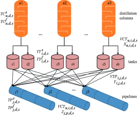
Figure 1. Schematic of blending and distribution infrastructure for diesel production. The text is organized as follows: in section 2 a
description of the problem addressed in this work is detailed. In section 3 the base model is presented. In section 4 three approaches are presented for addressing short term horizons and another approach is proposed for addressing long term horizons. Results and discussions are presented in section 5. Finally, the concluding remarks are brought up in section 6.
PROBLEM STATEMENT
The target problem involves a set of distillation units, which provide intermediate streams that are stored in dedicated storage tanks (Figure 1). Only cuts related to diesel production are in scope for the present problem. Taking into consideration that each distillation unit operates continuously and tanks cannot load and unload simultaneously, two run-down tanks are required for each distillation unit so that their cuts are available for composing the fi nal products at any time along the entire scheduling horizon. The quality of the content in each of the two rundown tanks is the same as that of the cut provided by its corresponding feeding unit and considered constant for the duration of the scheduling horizon as if the refi nery was developing a campaign imposed by planning, which is a reasonable assumption for short scheduling cycles. It is also assumed that the quality of the initial inventory in each of the intermediate tanks coincides with that of the underlying campaign, so that no mixing occurs at the run-down tanks.
F inished products are obtained by mixing the cuts produced by the distillation units, which are then sent through unidirectional pipelines to local markets. Each diesel grade is diff erentiated by two quality indicators; sulfur content and cetane number, which for simplicity are assumed to be determined as the weighted average of the volumes used of each cut. The blended products are pumped to the fi nal destinations without going through intermediate storage tanks, i.e., blending is done in-line prior to feeding pipelines. Full connectivity between tanks and pipelines is assumed. Pipelines operate independently and under unique demand requirements. Diesel parcels with diff erent grades are pumped contiguously, in which case an interface between two adjacent parcels establishes an undesirable interface containing off -spec material that demands appropriate handling.
The problem scope is as follows, given:
• The diesel related cuts produced by distillation units and their qualities;
• Initial intermediate material inventory; • Tank capacity;
• Pumping capacity;
• Product demand and specifi cations; • Time horizon.
Determine:
• Tank operations management and inventory profi le;
blended product for fulfilling demand and quality specifications;
• Pipeline operations schedule.
The objective function is to minimize costs, which include raw material, pumping, inventory costs as well as costs resulting from off-spec material generated at the interface in between blended diesel parcels transported through pipelines. The problem is subjected to the operating rules previously postulated.
MATHEMATICAL FORMULATION
Pinto et al. (2000) addressed the problem described in the problem statement and the complete model is presented next in detail with minor corrections. The mathematical model was built based on discrete time representation, which relies on a number of equally spaced time points resulting in an MILP model. The following nomenclature is used in the formulation presented in this section and in the studied approaches in the next section:
Indices and Sets
D set of days (d = {1, 2,…, D}) E set of events (e = {1, 2,…, E})
Ed set of events e that belong to each day d
EL
d set of events e that belong to each day d with the exception of the last event of each day
Ij subset of tanks i that can be aligned to pipeline j Iu subset of tanks i that can be loaded by distillation unit u J set of pipelines (j = {1, 2,…, J})
Ji subset of pipelines j that are allowed to connect to tank i K set of qualities (k = {1, 2,…, K})
P set of products (n,p = {1, 2,…, P}) T set of time intervals (t = {1, 2,…, T})
Td set of time periods t that belong to each day d U set of distillation units(u = {1, 2,…, DU})
Parameters
Cii inventory cost for tank i ($/m3)
Cpi cost associated with pumping intermediate material from tank i to pipeline ($/m3)
Crmi raw material cost associated with using intermediate material stored in tank i ($/m3)
Ctp,n cost associated with the interface established between products p and n ($) Dj,p demand of end product p incurred at pipeline j (m3)
Dj,p,t demand of product of each day) p incurred at pipeline j at time period t (m3) (usually incurred at the last time period Fmax
i maximum flowrate between distillation column and tank i (m 3/h)
Fmax
ij maximum pumping flowrate between tank i and pipeline j (m 3/h)
Fmax
j maximum pumping flowrate for pipeline j (m 3/h)
Fmin
i minimum flowrate between distillation column and tank i (m 3/h)
Fmin
ij minimum pumping flowrate between tank i and pipeline j (m 3/h)
Fmin
j minimum pumping flowrate for pipeline j (m 3/h)
H number of time periods (H = │T│)
NCi maximum number of connections between tank i and pipelines NTj maximum number of transitions allowed at pipeline j
T total length of time horizon (h) V0
i initial inventory in tank i (m 3)
Vimax maximum inventory allowed in tank i (m3)
Vimin minimum inventory allowed in tank i (m3)
ZDj,p 0-1 parameter that indicates if there is demand incidence for end product p at pipeline j
ZDj,p,t 0-1 parameter that indicates if there is demand incidence for end product p at pipeline j at time period t Continuous Variables
Fi,t inlet flowrate of tank i at time period t (m3/h)
Fj,p,t inlet flowrate of end product p to pipeline j at time period t (m3/h)
Fi,j,t flowrate between tank i and pipeline j at time period t (m3/h)
TE
j,p end time of loading end product p to pipeline j
TE
j,p,d end time of loading end product p to pipeline j within day d
Tj,e instant of time in which event e occurs in pipeline j TS
j,p start time of loading end product p to pipeline j
TS
j,p,d start time of loading end product p to pipeline j within day d
Vi,t inventory level at tank i in time period t (m3)
Binary Variables
Ej,p,e denotes if product p starts being pumped at event point e in pipeline j Pj,p,n indicates potential transition between product p and n on pipeline j
Sj,p,t denotes if operation of pipeline j is interrupted at time period t and the last product loaded to the pipeline was p
Sj,p,e denotes that no pumping operation is allocated to event point e in pipeline j and the last product loaded to the pipeline was p
Wj,p,n denotes if product n is pumped right after product p in pipeline j
Wj,p,n,e denotes if product n is pumped right after product pin pipeline j at event point e Xi,t denotes if tank i is being loaded at time period t
Yi,j,t denotes if tank i is loading pipeline j at time period t ZE
j,p,t denotes if end product p ends being loaded to pipeline j at time period t
ZE
,j,p,t,d denotes if product p ends being loaded to pipeline j at time period t within day d
Zj,p,t denotes if pumping of end product p to pipeline j is active at time period t ZS
j,p,t denotes if end product p starts being loaded to pipeline j at time period t
ZS
j,p,t,d denotes if product p starts being loaded to pipeline j at time period t within day d
As already mentioned, the objective function is to minimize costs, which include raw material, pumping, inventory as well as transition costs resulting from the
interface generated between blended diesel parcels transported through pipelines, which is mathematically stated in Equation 1.
The objective function is subject to the following constraints:
a) Material balance constraints
The total amount of material in each tank at each time
period is given by the initial inventory plus the amounts in and out of the tank accounted since the beginning of the time horizon, as given by Equation 2. In addition, constraint 3 sets upper and lower bounds to the inventory level.
(
)
, , , , , ,min
∈ ∈ ∈ ∈ ∈ ∈ ∈ ∈
+
+
+
∑∑∑
i i i j t∑∑
i i t∑∑∑
p n j p ni I j J t T i I t T j J p P n P
Crm
Cp F
Ci V
Ct W
(1), , ' , , ' '
,
≤ ∈
=
+
−
∀ ∈
∈
∑
∑
i
o
i t i i t i j t
t t j J
Equation 4 establishes the material balance between tanks and pipelines, which sets the amount of product p pumped through pipeline j equal to the consumed amount
of raw materials. Since at a given time t only one product p can be loaded to the pipeline j, the left hand side of Equation 4 has all terms null except for one.
Every product pumped through pipelines must satisfy quality requirements, which are guaranteed through
constraints 5a and 5b. In these constraints,
x
i k0, is a static parameter that represents the quality k of the raw materialstored in storage tank i, whereas
x
i kspc, is the specification value that the corresponding product must meet. Note that the quality calculation is a volume weighted average relationship, which can be assumed so because properties of raw materials are assumed to be constant for the duration of the scheduling horizon, which in turn means that density is also constant and thus cancelles out when put on bothsides of the equations. It must also be borne in mind that
the relationship between
F
j p t, , andF
i j t, , is establishedthrough Equation 4. If the assumption of a single campaign was not assumed, Equations 5 would assume a nonlinear form, making the problem more difficult to solve. This assumption is somewhat limiting but valid for short scheduling horizons. The sign on the inequality depends on the property under consideration. Sometimes a greater than or equal sign is used and sometimes the opposite is desired. In this paper, constraint 5a imposes a maximum amount on the sulfur content, while constraint 5b is used for imposing a minimum on the cetane number.
0
, , , , , ,
,
1,
∈ ∈
≥
∀ ∈
=
∈
∑
spc∑
p k j p t i k i j t
p P i I
x
F
x F
j
J k
t
T
(5a)0
, , , , , ,
,
2,
∈ ∈
≤
∀ ∈
=
∈
∑
spc∑
p k j p t i k i j t
p P i I
x
F
x F
j
J k
t
T
(5b)b) Demand constraint
Besides satisfying quality specifications, the total product volume produced must meet the demand, Equation 6. Although Equation 6 imposes the condition that demand
must be satisfied exactly, in the present work it will sometimes be allowed to dispatch an amount that is greater than the minimum required volume.
, , ,
,
∈
=
∀ ∈
∈
∑
j p t j pt T
F
D
j
J p
P
(6)c) Operating rules and logic constraints
Since distillation columns operate continuously, intermediate products are continuously transferred to either
of the available rundown tanks depending only on which tank is feeding a pipeline. At any time, however, only one rundown tank can receive the intermediate product from the distillation unit, as stated by Equation 7.
,
,
≤
≤
∀ ∈
∈
min max
i i t i
V
V
V
i
I t
T
(3), , , ,
,
∈ ∈
=
∀ ∈
∈
∑
∑
j
j p t i j t
p P i I
F
F
j
J t
T
(4)
,
1 ,
∈
= ∀ ∈
∈
∑
u
i t i I
In addition, it is forbidden for a tank to load and unload simultaneously. Therefore, at any time a tank is loading, unloading or settling. If a tank i is not being loaded (Xi,t = 0), then the maximum number of connections between tank i and pipelines
j
∈
J
i is given by NCi. On the otherhand, if a tank i is being loaded (Xi,t = 1), constraint 8 forbids unloading to any pipeline by setting all Yi,j,t = 0. Therefore, constraint 8 serves two purposes: it forbids simultaneous loading and unloading and at the same time limits the maximum number of connections between tanks and pipelines.
, , ,
,
∈
+
∑
≤
∀ ∈
∈
i
i i t i j t i
j J
NC X
Y
NC
i
I t
T
(8)Pinto et al. (2000) addressed a problem involving a very short time horizon. In that case, the heuristic that each product be shipped only once along the entire scheduling
horizon is operationally convenient. For that reason, constraint 9 limits the number of times each product is loaded to pipelines along the scheduling horizon.
, ,
1
,
∈
≤ ∀ ∈
∈
∑
Sj p t t T
Z
j
J p
P
(9)Once a pumping operation is started it must also be finished within the time horizon as given by Equation 10.
(
, , , ,)
0
,
∈
−
= ∀ ∈
∈
∑
S Ej p t j p t t T
Z
Z
j
J p
P
(10)Moreover, the time periods in which pumping has started and finished are identified by equations 11 and 12, respectively. It should be noted that, because of constraints 9 and 10, only one of the ZSj,p,t in the summation on the right hand side of equation 11 will be nonzero. Likewise,
only one of the ZEj,p,t in the summation on the right hand side of equation 12 will be nonzero. The inequality 13 ensures that the start of pumping will be no later than its end.
,
.
, ,,
∈
=
∑
∀ ∈
∈
S S
j p j p t
t T
T
t Z
j
J p
P
(11),
.
, ,,
∈
=
∑
∀ ∈
∈
E E
j p j p t
t T
T
t Z
j
J p
P
(12),
≤
,∀ ∈
,
∈
S E
j p j p
T
T
j
J p
P
(13)Equation 14 sets the time interval in which product p is being pumped. Zj,p,t= 1 means that pumping of product p is active in time period t on pipeline j. Equation 14 sets the time-period interval in which product p is being blended
and shipped. Equation (10) together with equation (14) prevents the situation where a product would start shipment and, before its completion, another product would start being shipped to the same pipeline.
, , , , ' , , ' '
, ,
≤ ′<
=
∑
S−
∑
E∀ ∈
∈
∈
j p t j p t j p t
t t t t
Z
Z
Z
j
J p
P t
T
(14)If a tank is loading to a pipeline, then one of the products p is being pumped, as stated by constraint 15. In addition, for a given pipeline and a given time period at most one of
, , , ,
,
,
∈
≤
∑
∀ ∈
∈
∈
i j t j p t p P
Y
Z
i
I j
J t
T
(15), ,
1 ,
∈
≤ ∀ ∈
∈
∑
j p t p PZ
j
J t
T
(16)d) Flowrate constraints
Constraints 17, 18 and 19 impose limits to flowrate
between column and tanks, between tanks and pipelines and through pipelines, respectively.
,
≤
,≤
,∀ ∈
,
∈
min max
i i t i t i i t
F
X
F
F
X
i
I t
T
(17), , ,
≤
, ,≤
, , ,∀ ∈
,
∈
,
∈
min max
i j i j t i j t i j i j t
F
Y
F
F
Y
i
I j
J t
T
(18), ,
≤
, ,≤
, ,∀ ∈
,
∈
,
∈
min max
j j p t j p t j j p t
F
Z
F
F
Z
i
I p
P t
T
(19)e) Transition constraints
Transitions are known as the interfaces created between parcels of different products pumped consecutively through
the same pipeline. Constraints 20 and 21 are complementary to each other and are used to identify potential transitions, given that each product is allowed to be pumped only once throughout the entire scheduling horizon.
, ,
, ,
, ,
,
−
≥
∀ ∈
∈
≠
S S
j n j p j p n
T
T
P
j
J
p n
P
p
n
T
(20)
(
1
, ,)
, ,, ,
,
−
−
≤
S−
S∀ ∈
∈
≠
j p n j n j p
T
P
T
T
j
J
p n
P
p
n
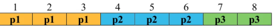
(21)A sample schedule is used to illustrate the application of the constraints 20 and 21. Three products, p1, p2 and
p3 are pumped through pipeline j along a time horizon composed of 8 discrete time-periods as given by Figure 2. Pumping of product p1 starts at time-period 1 and finishes
at time-period 3, pumping of product p2 starts at time period 4 and finishes at time-period 6, whereas pumping
of product p3 starts at period 7 and finishes at
time-period 8. Therefore, , 1
=
1
S j p
T
, , 1
=
3
E j p
T
, , 2
=
4
S j p
T
,
, 2
=
6
E j p
T
, , 3
=
7
S j pT
and , 3
=
8
E j pT
. It should be noted that transitions are established between products p1 and
p2 and between p2 and p3. However, there is no transition between p1 and p3, p2 and p1, p3 and p1 and p3 and p2.
Figure 2. Schedule involving pumping of three products (p1, p2 and p3) through a pipeline along a time horizon comprised of eight discrete time periods.
1
2
3
4
5
6
7
8
Table 1. onstraints 20 and 21 reflecting the sample schedule of Figure 2.
Constraint 20 Constraint 21 Pj,p,n
p1, p2
P
j, 1, 2p p≥
(
4 1 / 8
−
)
=
3 / 8
−
8 1
(
−
P
j, 1, 2p p)
≤ − =
4 1
(
)
3
1p1, p3
P
j, 1, 3p p≥
(
7 1 / 8
−
)
=
6 / 8
−
8 1
(
−
P
j, 1, 3p p)
≤ − =
7 1
(
)
6
1p2, p1
P
j, 2, 1p p≥ −
(
1 4 / 8
)
= −
3 / 8
−
8 1
(
−
P
j, 2, 1p p)
≤ −
1 4
(
)
= −
3
0p2, p3
P
j, 2, 3p p≥
(
7 4 / 8
−
)
=
3 / 8
−
8 1
(
−
P
j, 2, 3p p)
≤ −
7 4
(
)
=
3
1p3, p1
P
j, 3, 1p p≥ −
(
1 7 / 8
)
= −
6 / 8
−
8 1
(
−
P
j, 3, 1p p)
≤ −
1 7
(
)
= −
6
0p3, p2
P
j, 3, 2p p≥
(
4 7 / 8
−
)
= −
3 / 8
−
8 1
(
−
P
j, 3, 2p p)
≤ −
4 7
(
)
= −
3
0Constraints 20 and 21 are created for all combinations of p1, p2 and p3 as presented in Table 1. Note that the last column in the Table refers to the resulting values assumed by the variable Pj,p,n when constraints 20 and 21 are simultaneously satisfied. The purpose of those constraints is to indicate potential transitions. For this reason, besides indicating the actual transitions between products p1 and
p2 and between products p2 and p3, transition between products p1and p3 is also indicated as a potential one. Consequently, additional constraints must be introduced in order to screen out transitions that are not actual. However, before presenting the additional constraints, it must be emphasized that there is no transition when product n equals product p, as postulated by Equation 22.
, ,
=
0
∀ ∈
, ,
∈
,
=
j p n
P
j
J
p n
P
p
n
(22)Since each product can be handled only once along the entire time horizon and knowing that products for which there is no demand will not be shipped through pipelines (equation 6), it is possible to predict the total number of transitions at each pipeline. The total number of transitions
will be equal to the total number of products for which there is demand diminished by 1 or null if demand is incurred for only one product, Equation 23. Note that Equation 23 is not part of the model but just the way parameter NTj is calculated and used as an input parameter to the model.
,
1, 0
∈
=
−
∀ ∈
∑
j j p
p P
NT
max
ZD
j
J
(23)where,
ZD
j p, indicates if there is demand incidence forproduct p at pipeline j. The input parameter NTj is used to
define the actual total number of transitions allowed to be identified by the model, as given by Equation 24.
, ,
∈ ∈
=
∀ ∈
∑∑
j p n jp P n P
W
NT
j
J
(24)
Variable Wj,p,n assumes 1 if the actual transition is identified and 0 otherwise and it is upper bounded by Pj,p,n determined by constraints 20 and 21. If there is no potential feasibility for the occurrence of a transition between
, ,
≤
, ,∀ ∈
, ,
∈
j p n j p t
W
P
j
J
p n
P
(25)As discussed before, constraints 20 and 21 usually indicate a number of potential transitions that is greater than or equal to the total number of the actual transitions.
Therefore, constraints 26 and 27 are added to screen out invalid transitions and to allow transitions between products p and n (or n and p) to occur only once.
, , ,
,
∈
≤
∀ ∈
∈
∑
j p n j pn P
W
ZD
j
J
p
P
(26), , ,
,
∈
≤
∀ ∈
∈
∑
j p n j np P
W
ZD
j
J
n
P
(27)Constraints 26 and 27 only allow transitions involving product p or n if there is demand incidence for them. In the model proposed by Pinto et al. (2000), the right hand side of constraints 26 and 27 was set to 1 instead of ZDj,p/ ZDj,n. That modification was necessary because, if there was no demand for a product, a value 1 on the right hand side of constraints 26 and 27, instead of ZDj,p/ZDj,n, could produce an erroneous transition identification, as we indeed found out.
In order to demonstrate the idea on how the set of
constraints 26 and 27 work, we take again the example of Figure 2 and the potential candidates indicated in Table 1: [(p1, p2), (p1, p3), (p2, p3)]. The total number of transitions calculated by equation 23 is 2, which is used in constraint 24. Now, writing constraints 26 and 27 explicitly for all combinations of p and n we get Equations 26a-c and 27a-c shown in Table 2 as the individual constraints generated from constraint 26 and 27 defined over their domain, respectively.
Table2. Constraints 26 and 27 reflecting the sample schedule of Figure 2.
Constraint 26 Constraint
p1
W
j, 1, 1p p+
W
j, 1, 2p p+
W
j, 1, 3p p≤
1
(26a) p2W
j, 2, 1p p+
W
j, 2, 2p p+
W
j, 2, 3p p≤
1
(26b)p3
W
j, 3, 1p p+
W
j, 3, 2p p+
W
j, 3, 3p p≤
1
(26c) Constraint 27p1
W
j, 1, 1p p+
W
j, 2, 1p p+
W
j, 3, 1p p≤
1
(27a) p2W
j, 1, 2p p+
W
j, 2, 2p p+
W
j, 3, 2p p≤
1
(27b)p3
W
j, 1, 3p p+
W
j, 2, 3p p+
W
j, 3, 3p p≤
1
(27c)From 26a, either transition [(p1,p2), (p1,p3)] is feasible. From 26b only transition (p2,p3) is possible, whereas 27b allows only (p1,p2) and by 27c either of the transitions [(p1,p3), (p2,p3)] is allowed. Therefore, the only solution that satisfies simultaneously 20-22 and 24-27 is the pair [(p1,p2), (p2,p3)], having in mind that the total number of transitions that must be identified is 2.
A quick analysis of the just presented model lead us to conclude that this model, as is, cannot be readily applied to represent real-world problems encompassing a few days
STUDIED APPROACHES
Transitions arise naturally in scheduling problems and have been modeled and discussed in a number of PSE papers (Karamarkar and Schrage, 1985; Sahinidis and Grossmann, 1991; Kondili et al., 1993; Lee at al., 1996; Wolsey, 1997; Mendez et al., 2006; Kelly and Zyngier, 2007; Liu et al, 2010; Harjunkoski et al., 2014). Two contributions are worth bringing up in more details; Kondili et al. (1993), using the discrete time representation, introduced a mechanism for identifying transitions that relies on the evaluation of any two time-periods, as opposed to the traditional form in which only consecutive time-periods are evaluated (Lee at al., 1996). Kelly and Zienger (2007) proposed an alternative approach that uses auxiliary non-integer variables capable of producing tighter relaxation problems and thus resulting in a much more efficient approach than that of Kondili and coworkers.
In this section, two formulations are derived from the base model, which result from replacing the set of constraints that are used for identifying transitions by the two most common forms found in the literature, which
consider evaluation of any two time-periods and evaluation of consecutive time-periods. The resulting formulations encompass very short time horizons in the same fashion as the base model. In that case, the adopted heuristic which dictates that products are handled only once at each pipeline is kept in the formulations without any hurdle. A new approach is then introduced that takes into consideration characteristics of the two classic forms of identifying transitions. Results obtained with the three formulations are compared and discussed in the results section. Next, attention is turned in the direction of problems addressing longer time horizons. In this case, improvements for the introduced approach are proposed that rely on use of two time scales, in which one can be derived as the aggregation of the other. The following sections are organized so that the discussion is concentrated in two different fronts; formulations for short-term time horizons and formulation for long-term time horizons. The complete set of equations that compose each optimization problem presented in the following sections are summarized in Appendix A1-A4. In all problems that follow, the objective function is given by Equation 28.
(
)
, , , , , , , ,min
∈ ∈ ∈ ∈ ∈ ∈ ∈ ∈ ≠ ∈
+
+
+
∑∑∑
i i i j t∑∑
i i t∑∑ ∑ ∑
p n j p n ei I j J t T i I t T j J p P n P p n e E
Crm
Cp F
Ci V
Ct W
(28)Short-Term Time Horizon
Model 1
In the first approach, the variable Pj,p,n together with constraints 20-22 and 25-27 are dropped from the base
model, which are replaced by constraint 29. This constraint has been extensively used in optimization formulations for identifying transitions between tasks occurring in consecutive time-periods (see for example Lee at al., 1996).
, ,
≥
, ,+
, , 1+− ∀ ∈
1
, ,
∈
,
∈
,
≠
j p n j p t j n t
W
Z
Z
j
J
p n
P t
T p
n
(29)The reader should notice that 29 causes an expressive increase in the number of constrains, since an equation is created for every (p,n) combination between two time
periods, t and t+1, with
p
≠
n
. On the other hand, there is also a reduction in the number of constraints and variables by dropping constraints 20-22 and 25-27 and variables Pj,p,n.There is an evident flaw in this approach in that constraint 29 is only capable of identifying transitions in cases where different tasks are allocated to adjacent time-periods. Therefore, it is not of practical use unless allocation is enforced for every time-period or if idle time periods are not intermediary ones. In spite of that, this approach is kept in our studies for sake of comparison with other approaches.
Model 2
scheduled in between the time-periods under evaluation and thus Wj,p,n = 1 will be enforced given that p is allocated to t and n is allocated to t’. If, on the other hand, at least one task is scheduled in between t and t’, the third term on
the right hand side of 30 will result in an integer number, leading to the relaxation of the constraint, regardless of the allocations in t and t’.
1 , , , , , , , ,
1
1
, ,
,
,
′
′ ′ ′′
′∈ ′′= + −
≥
+
−
∑ ∑
t− ∀ ∈
∈
∈
≠
j p n j p t j n t j p t
p Pt t
W
Z
Z
Z
j
J p n
P t
T p
n
(30)An apparent drawback of constraint 30 in comparison to 29 is the total number of constraints necessary for creating all combinations of (t, t´) and (p,n). Note that for each t, t’ will be varied from t + 1 to the last time-period of the scheduling horizon and hence creating a huge number of constraints.
Figure 3 illustrates the use of constraint 30 in one such example where the pumping operation for product p1 is scheduled to start in the first time-period and to end in the fourth time period. Pipeline operation is then temporarily interrupted for the next two time-periods. Pumping of product p2 is initiated in the seventh time-period and
continues until the end of the schedule horizon. In Table 3, constraint 30 is illustrated for t = 4, with t’ varying from 5 to 8, p = p1 and n = p2. It should be noted that, for t’ = t + 1 (adjacent time periods), 30 assumes the form of constraint 29. It is also demonstrated that 30 is able to handle pumping interruption and still identify transitions correctly. It must be borne in mind that constraint 30 works in synchronization with the objective function in that Wj,p,n = 1 incurs transition costs. Therefore, Wj,p,n will be pushed down to zero by the objective function in case constraint 30 does not impose that Wj,p,n =0.
Figure 3. Schedule involving pumping of two products (p1 and p2) through a pipeline along a time horizon comprised of ten discrete time periods.
Table 3. Constraints 30 reflecting the sample schedule of Figure 3.
Constraint 30 Wj,p1,p2 Constraint
, 1, 2
≥
, 1,4+
, 2,5−
1
j j j
W
p pZ
pZ
p 0 (30a)(
) (
)
, 1, 2
≥
, 1,4+
, 2,6−
, 1,5−
, 2,5−
1
j j j j j
W
p pZ
pZ
pZ
pZ
p 0 (30b)(
) (
)
, 1, 2
≥
, 1,4+
, 2,7−
, 1,5+
, 1,6−
, 2,5+
, 2,6−
1
j j j j j j j
W
p pZ
pZ
pZ
pZ
pZ
pZ
p 1 (30c)(
) (
)
, 1, 2
≥
, 1,4+
, 2,8−
, 1,5+
, 1,6+
, 1,7−
, 2,5+
, 2,6+
, 2,7−
1
j j j j j j j j j
W
p pZ
pZ
pZ
pZ
pZ
pZ
pZ
pZ
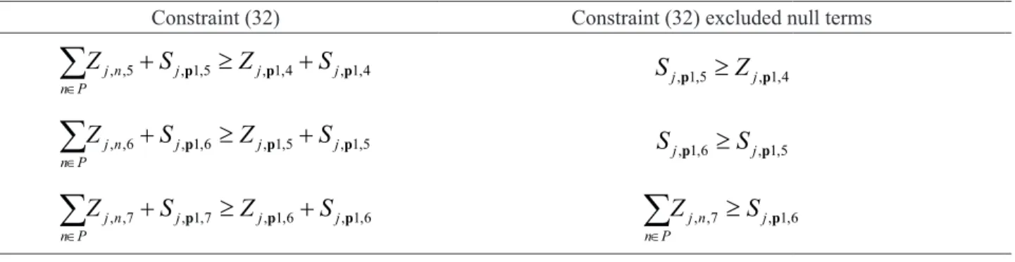
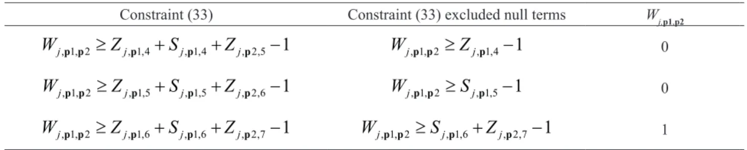
p 0 (30d)Table 4. Constraints 32 and 33 reflecting the sample schedule of Figure 3.
Constraint (32) Constraint (32) excluded null terms
, ,5 , 1,5 , 1,4 , 1,4
∈
+
≥
+
∑
j n j j jn P
Z
S
pZ
pS
p, 1,5
≥
, 1,4j j
S
pZ
p, ,6 , 1,6 , 1,5 , 1,5
∈
+
≥
+
∑
j n j j jn P
Z
S
pZ
pS
p, 1,6
≥
, 1,5j j
S
pS
p, ,7 , 1,7 , 1,6 , 1,6
∈
+
≥
+
∑
j n j j jn P
Z
S
pZ
pS
p , ,7 , 1,6∈
≥
∑
j n jn P
Z
S
p1
2
3
4
5
6
7
8
9
10
Constraint (33) Constraint (33) excluded null terms Wj,p1,p2
, 1, 2
≥
, 1,4+
, 1,4+
1
, 2,5−
j j j j
W
p pZ
pS
pZ
pW
j, 1, 2p p≥
Z
j, 1,4p−
1
0, 1, 2
≥
, 1,5+
, 1,5+
1
, 2,6−
j j j j
W
p pZ
pS
pZ
pW
j, 1, 2p p≥
S
j, 1,5p−
1
0, 1, 2
≥
, 1,6+
, 1,6+
1
, 2,7−
j j j j
W
p pZ
pS
pZ
pW
j, 1, 2p p≥
S
j, 1,6p+
1
Z
j, 2,7p−
1Model 3
If on the one hand constraint 29 is simple and easy to apply, on the other hand it is not able to identify transitions if allocation of intermediary time-periods is vacant. Constraint 30 is able to circumvent the downside of constraint 29 but at the expense of an increase in the number of constraints, which affect computational performance. We propose a third approach that is conceptually similar to the first approach in that only consecutive time-periods are evaluated but some kind of mechanism needs to be added to address the case of idle time-periods. The solution found was to keep track of the history on the last product loaded to the pipeline, in case the pipeline operation is interrupted temporarily. That information is then used to correctly
identify transitions under any circumstances. This idea of using memory variables has been used by other researchers in the past (Kelly and Zyngier, 2007), but our formulation is completely different.
In order to be able to track history, a new variable is introduced, Sj,p,t, which assumes 1 if operation of pipeline j is interrupted at time period t and the last product loaded to the pipeline was p. In the context of the pipeline operation schedule, at any point in time a pipeline might be either pumping a single product or idle, as stated in Equation 31. The second summation on the left hand side of the equation will be nonzero if the pipeline operation was interrupted in time-period t and one of the products p was the last product injected into the pipeline sometime in the past.
, , , ,
1 ,
∈ ∈
+
= ∀ ∈
∈
∑
j p t∑
j p tp P p P
Z
S
j
J t
T
(31)Constraint 32 identifies the exact time-period in which the last injection was done. If product p is shipped in time-period t, Zj,p,t = 1 and Sj,p,t = 0 by 31. If operation is
interrupted in the following time period ∈ , , 1+
0
=
∑
j n t n PZ
in constraint 32, which then enforces Sj,p,t+1 = 1, meaning that the information on p as the last loaded product will be carried over. If the pipeline remains static for more than
one time-period Sj,p,t will repeatedly pass the information on to Sj,p,t+1 until pipeline operation is recovered or the end of the scheduling horizon is reached. Transition is then easily identified by evaluating adjacent time-periods according to constraint 33. Note that the only difference between constraints 29 and 33 is the introduction of Sj,p,t on the right hand side. However, this constraint works in coordination with constraints 31 and 32.
{ }
, , 1+ , , 1+ , , , ,
,
, T
∈
+
≥
+
∀ ∈
∈
∈ −
∑
j n t j p t j p t j p tn P
Z
S
Z
S
j
J p
P t
T
(32){ }
, ,
≥
, ,+
, ,+
, , 1+− ∀ ∈
1
, ,
∈
,
∈ −
T ,
≠
j p n j p t j p t j n t
W
Z
S
Z
j
J
p n
P t
T
p
n
(33)Constraints 31 and 32 are illustrated with the example of Figure 3 (Table 4) along time-periods 4, 5 and 6 comprising the time interval in which the pipeline operation is interrupted. Constraint 32 is written only for product p1, whereas constraint 33 is written for the transition identification between products p1 and p2, which is effectively done even with the pipeline remaining without operation for two consecutive time-periods.
Long-Term Time Horizon
are used to screen out non-existing transitions potentially identified by constraints 20 and 21.
In principle, for long time horizons, the idea that products are shipped only once along the entire time horizon cannot be sustained since multiple shipments are unavoidable because demand is distributed along the time horizon and pipelines are capacitated. In other words, there may be multiple due dates for the same product and, most likely, it will not always be possible to lump parcels so as to fulfill multiple demand incidences because of pumping capacity. On the other hand, enforcing a maximum number of shipments for each product establishes the maximum number of events or shipments that may happen within a time interval, which sets an upper bound on the number of transitions. In order to take advantage of this fact, the idea was to create two levels of granularity for time, e.g., the scheduling horizon could be subdivided in days within which products could be allowed to be shipped only once, which in turn could be subdivided in hours to accommodate allocation of multiple time periods. Bottom line, with the two levels of aggregation, transitions would be managed on a higher level of detail and hence a few constraints would be required to create all combinations of product interfaces and product allocation would be managed on the lower level of aggregation.
As to the second heuristic in which the total number of transitions is known beforehand, under no conditions could it be sustained in longer scheduling horizons because shipment of products could be anticipated, including products for which there was no demand in previous days. As long as there was available free capacity, anticipation would be possible. Shipment of products with zero demand could be convenient in cases of pipelines that transport multiple products and require more flexibility in terms of product sequencing. In that case, a small volume of a product with no demand could be injected in between products that would otherwise not be allowed to be put in contact with each other, which is sometimes a common
practice.
In the previous section three different approaches were considered, all of which involve replacement of constraints 20-22 and 25-27 by other forms of transition identification. As already stated and, as will be demonstrated by the results presented below, the first approach is not robust enough to address scenarios where interruptions are scheduled between shipments. The second approach produces models with dimensions that grow very quickly with the scheduling horizon. The third approach was then readjusted to incorporate the time aggregation scheme mentioned previously so that that approach can be extended to cases where longer time horizons are considered.
Model 4
In this approach, the fundamental premise that each product can be shipped only once at each pipeline is retained in the model, not for the entire scheduling horizon but for a predefined set of time-periods. The scheduling horizon is subdivided into two levels of granularity. In the lowest level, the scheduling horizon is split in time-periods representing hour buckets. Time-time-periods are then aggregated in day buckets. There is a subset of time-periods
that belongs to each day (
t
∈
T
d), as illustrated in Figure 4. With this bi-level time representation, it is imposed that the same product cannot be shipped more than once within the same day. Note also, by the scheme presented in Figure 4, that event points are created to either indicate points in time in which the start of new shipments is scheduled or the start of a new day. The number of event points within each day must equal the number of products and the total number of event points must be │E│=│P│.│D│. Asubset of event points is allocated to each day in increasing
order (
e
∈
E
d) so that the event point subsets are mutually exclusive. With that framework, transitions are identified by comparing adjacent events e and e+1, even if they belong to different days.Figure 4. Event point - bilevel time representation.
1 2 3 4 21 22 23 24 25 26 27 28 45 46 47 48 49 50 51 52 69 70 71 72
d
1d
2d
3e
1e
2e
3e
4e
5e
6e
7e
8e
9e
10Most of the constraints indexed in time remain unchanged. The only constraints that are impacted by the new time representation are those representing operating rules used for ensuring that there will be single movements for each product within the same day. Therefore,
constraints 34-38 are the equivalent of Equations 9-12 and 14 indexed only in time-periods, which represent hours. Constraint 13 is replaced by Equation 39 to ensure that the end of pumping will be equal to its start plus the pumping duration.
, , ,
1
,
,
∈
≤ ∀ ∈
∈
∈
∑
d
S j p t d t T
Z
j
J p
P d
D
(34)(
, , , , , ,)
0
,
,
∈
−
= ∀ ∈
∈
∈
∑
d
S E
j p t d j p t d t T
Z
Z
j
J p
P d
D
(35), ,
.
, , ,, ,
∈
=
∑
∀ ∈
∈
∈
d
S S
j p d j p t d t T
T
t Z
j
J p
P d
D
(36), ,
.
, , ,, ,
∈
=
∑
∀ ∈
∈
∈
d
E E
j p d j p t d t T
T
t Z
j
J p
P d
D
(37)
, , , , ,′ , , '
, ,
,
′≤ ′<
=
∑
S−
∑
E∀ ∈
∈
∈
∈
j p t j p t d j p t d d
t t t t
Z
Z
Z
j
J p
P t
T d
D
(38), , , , , ,
1 ,
,
,
∈
=
+
−
∀ ∈
∈
∈
∑
d
E S
j p d j p d j p t t T
T
T
Z
j
J p
P d
D
(39)Equation 6 must be decomposed into two equations if demand is to be met exactly. Equation 40a guarantees that demand is satisfied at due dates, whereas 40b enforces that the total amount of product p shipped along the scheduling horizon must exactly meet demand. Note that products with
no demand are allowed to be shipped since constraint 40b is applied only for those products with non-zero demand. If the total volume transferred of each product were allowed to be greater than the total demand, 40b would be modified with a corresponding greater than or equal sign.
, , ´ , , ´ ´ ´
,
,
,
1
≤ ≤
≥
∀ ∈
∈
∈
>
∑
j p t∑
j p t jt t t t
F
D
j
J p
P t
T NT
(40a), ,
=
, ,∀ ∈
,
∈
,
∈
∑
j p t∑
j p tt t
F
D
j
J p
P t
T
(40b)The start of a pumping operation must match an event point, which is done through Equation 41. The instant of time in which the event occurs must exactly match the start of the pumping operation, (constraints 42 and 43).
, , , , ,
,
,
∈ ∈=
∀ ∈
∈
∈
∑
∑
d d S j p e j p t de E t T
E
Z
j
J p
P d
D
(41)(
)
,
≥
, ,−
1
−
, ,∀ ∈
,
∈
,
∈
,
∈
S
j e j p d d j p e d
T
T
H
E
j
J p
P e
E d
D
(42)(
)
,
≤
, ,+
1
−
, ,∀ ∈
,
∈
,
∈
,
∈
S
j e j p d d j p e d
T
T
H
E
j
J p
P e
E d
D
(43)Event points must be monotonically non-decreasing, since adjacent event points are used in transition
,
≥
,−1∀ ∈
,
∈
j e j e
T
T
j
J e
E
(44)There might be event points to which no pumping operation will be allocated. With the intent of avoiding the occurrence of symmetric solutions, constraint 45 is added. By introducing such a constraint, pumping operations will be always forced to be allocated to the first events of each day, which has a direct impact on computational performance.
, , , ,+1
,
,
∈ ∈
≥
∀ ∈
∈
∈
∑
∑
Lj p e j p e d
p P p P
E
E
j
J d
D e
E
(45)Transitions are identified considering only consecutive event points, instead of consecutive time-periods, which drastically reduces model size in comparison to the case where time-periods are used. The set of constraints involved in transition identification is similar to that proposed in model 3. The only difference is that, instead of time-periods, event points are considered (constraints 46-48).
, , , ,
1
,
∈ ∈
+
=
∀ ∈
∈
∑
j p e∑
j p ep P p P
E
S
j
J e
E
(46){ }
, ,+1 , ,+1 , , , ,
,
,
E
∈
+
≥
+
∀ ∈
∈
∈ −
∑
j n e j p e j p e j p en P
E
S
E
S
j
J p
P e
E
(47){ }
, , ,
≥
, ,+
, ,+
, ,+1− ∀ ∈
1
, ,
∈
,
∈ −
E ,
≠
j p n e j p e j p e j n e
W
E
S
E
j
J
p n
P e
E
p
n
(48)The complete model is presented in Appendix A4.
NUMERICAL RESULTS
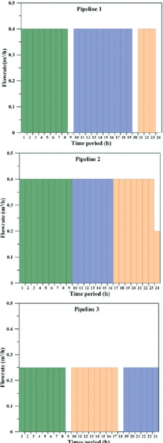
The problem presented in Pinto et al. (2000) was used, with minor changes, for illustrating the application of the first three approaches, which comprises a very short-term time horizon comprised of 24 uniform time-periods of 1 hour. A derivation of that example was also used to illustrate the application of the extended approach, which comprises a time horizon of 4 days (96 hours). For the short-term schedule, the volume injected into the pipeline is allowed to be greater than demand, which is incurred only at the end of the time horizon, whereas demand is distributed along the time horizon for the extended one with incurrence at the end of each day. Demand data are given in Table 5. Three distillation columns produce intermediate products with different constant properties, which are stored in dedicated tanks. The input data related to distillation columns, rundown tanks and pumping capacities are given in Table 6. The intermediate products are blended in-line to produce diesel with three different specs (Table 7) and dispatched through three pipelines. Full connectivity is assumed. Dependent transition costs are given in Table 8.
All formulations resulted in MILP problems which were coded using the GAMS 24.4 system and solved by
CPlex 12 on an Intel(R) Core(TM)i7, CPU3.5 GHz and 16.0GB RAM. The relative gap was set to 0.01% as one of the termination criteria for the approaches involving short-term time horizons and 0.1% or 3,600 CPU seconds for the approach encompassing longer time horizon.
Short-Term Time Horizon
The computational results for all approaches encompassing short-term time horizons are presented in Table 9, from which it can be noticed that the first and second approaches contain less binary variables than the base model since the variable Pj,p,n was dropped in the new approaches. However, the introduction of Sj,p,t variable in the third approach contributed to a slight increase in the number of binary variables.