Clustering of variables with a three-way approach for health sciences

H

ELENA

B

ACELAR

-N

ICOLAU

UNIVERSITY OF LISBON

F

ERNANDO

C

OSTA

N

ICOLAU

NEW UNIVERSITY OF LISBON

Á

UREA

S

OUSA

UNIVERSITY OF THE AZORES

L

EONOR

B

ACELAR

-N

ICOLAU

UNIVERSITY OF LISBON

Cluster analysis or classification usually concerns a set of exploratory multivariate data analysis methods and techniques for grouping either a set of statistical data units or the associated set of descrip-tive variables, into clusters of similar and, hopefully, well separated elements. In this work we refer to an extension of this paradigm to generalized three-way data representations and particularly to classifi-cation of interval variables. Such approach appears to be especially useful in large data bases, mostly in a data mining context. A health sciences case study is partially discussed.

Key words: Three-way data; Interval variable; Cluster analysis of variables; Similarity coefficient; Hi-erarchical clustering model.

Correspondence concerning this article should be addressed to Helena Bacelar- icolau, Universidade de Lisboa, Faculdade de Psicologia, LEAD, Alameda da Universidade, 1649-013 Lisboa, Portugal. Email: hbacelar@psicologia. ulisboa.pt

Cluster analysis or classification usually concerns exploratory multivariate data analysis methods and techniques for grouping either a set of statistical data units (individuals, cases, …) or an associated set of descriptive variables, into clusters of similar elements, hopefully homogenous and well separated. In this work we refer to a generalization of this paradigm that appears to be particularly useful (but not only) when large data bases are used, mostly in a data mining context: classification/clustering of generalized three-way or complex data instead of the more common two-way data approach. Hierarchical clustering methods are based on the affinity coefficient and on some empirical aggregation criteria as well as probabilistic aggregation criteria. These are is-sued from an adaptive (parametric) family of aggregation criteria.

Concerning applications, individuals which belong to three different groups and variables which correspond to psychological scales, are analyzed in this study. The aim was first of all to ana-lyze the underlying clustering structures of groups, separately, and to compare them. Hence, cluster analysis of each group was based on the usual two-way data representation of a matrix crossing the

set of individuals with the set of variables. Additionally we searched for a reference global cluster-ing structure over the whole sample, able to keep the variability of the groups. Thus in this case the corresponding data base should include not only the two sets of individuals and variables but also the groups set. Moreover, groups might have different dimensions or alternatively be represented by interval data. Therefore such a global cluster analysis should be based on a generalized three-way or complex data representation (H. Bacelar-Nicolau, 2002; H. Bacelar-Nicolau, Nicolau, Sousa, & L. Bacelar-Nicolau, 2009; Souza & De Carvalho, 2004). The present work refers to global cluster analysis. In order to obtain data typologies, hierarchical cluster analysis methods were ap-plied to classify the set of variables/scales, using a suitable extended affinity coefficient (e.g., Matu-sita, 1951, 1955; H. Bacelar-Nicolau, 2002; Nicolau & Bacelar-Nicolau, 1982) as a proximity measure associated with four different aggregation criteria: two empirical ― single link and com-plete link ― and two probabilistic criteria ― Aggregation Validity Link (AVL) and Aggregation Validity B-Link (AVB) (B from Bacelar-Nicolau, 1985, meaning also Brake that is “reducing both chain and symmetry/equicardinality clustering effects”; e.g., Bacelar-Nicolau, 1988; Lerman, 1972, 1981). The single link and the two probabilistic criteria are incorporated into an adaptive family of aggregation criteria similar to Lance and Williams’ well known formula (e.g., H. Bacelar-Nicolau, 2002; Lerman, 1981; Nicolau & Bacelar-Nicolau, 1998). Part of the three-way or complex cluster-ing approach was published and programmed in Bock and Diday (2000) and associated software SODAS, as well as in H. Nicolau (2000, 2002), L. Nicolau (2002), H. Bacelar-Nicolau et al. (2009, 2010), and Sousa (2005). Applications have been reported in those papers as well as, for instance, in H. Bacelar-Nicolau (2002), Nicolau et al. (2007), Sousa, Nicolau, H. Bace-lar-Nicolau, and Silva (2010), Sousa, Tomás, Silva, and H. Bacelar-Nicolau (2013).

The next section provides an overview of the extended three-way clustering approach based on the generalized affinity coefficient, adapted to the real data base and clustering aims referred to in the case study, where the application of the methodology to psychological data issued from the Par-enting Stress Index (PSI; Abidin, 1997) questionnaire is illustrated.

WEIGHTED GENERALIZED AFFINITY

AND ASYMPTOTIC PERMUTATION STANDARDIZED COEFFICIENTS

Let D be a set of individuals (first-order statistical data units), described by a set V of p variables. Individuals are split into n different groups (second-order statistical data units), with same or different cardinals. Here we are concerned with hierarchical clustering models on the set of variables/scales. Therefore the global data table to work with is composed by n sub-tables repre-senting groups Gj (j = 1,…,n), where columns correspond to variables Vk (k = 1,...,p) and rows (ℓ =

1,...,mj) of each j-th sub-table describe Gj individuals (Table 1).

The Basic Affinity Coefficient

The affinity coefficient was introduced by Matusita in 1951 to measure proximity between two distribution functions (Matusita, 1951, 1955). Matusita studied affinity properties and ap-plications in a number of important papers, mostly in an inferential statistics context. The affinity

TABLE 1

Generalized three-way data matrix

V1 ··· Vp Group G1 1 x111 ··· x1p1 . . . . . . m1 x11m1 ··· x1 pm1 Total x11• _··· x1p• . . . . . . . . . Group Gn 1 xn11 ··· xnp1 . . . . . . mn xn1mn ··· xnpmn Total xn1• ··· xnp•

coefficient is related to a special case of the Hellinger distance, also designated as the Bhat-tacharyya distance (e.g., H. Bacelar-Nicolau, 2000; Bock & Diday, 2000; Domenges & Volle, 1979; Nikulin, 2001). We have extensively studied the affinity coefficient in a cluster analysis context frequently regarding classification of variables, for instance when searching for typolo-gies in multivariate analysis of data from human sciences. Furthermore exploratory empirical as well as probabilistic clustering methods/models based on the affinity coefficient have been de-veloped for classification of variables. Later on the affinity coefficient was extended to clustering of statistical data units, mainly in a three-way approach (e.g., H. Bacelar-Nicolau, 1988, 2000, 2002; H. Bacelar-Nicolau et al., 2009, 2010).

Let V be a set of p variables, describing a set D of statistical data units, so that each of the ×p cells of the corresponding data table X contains one single non-negative real value xik (i =

1,..., ; k = 1,...,p) which is the value of the k-th variable on the i-th individual. This applies for instance to cluster analysis of each group Gj above, with = mj (j = 1,…,n). The basic affinity

coefficient a

(

k, k'

)

between Vk and Vk' variables (k, k' = 1,…,p), is defined by:

(

)

_∑

₌ • • ⋅ = _i k ik k ik x x x x k k a ₁ ' ' ' , , where x•k =

∑

_i=1xik and x•k' =

∑

_i=1xik' (1) Therefore the basic affinity coefficient between two such -dimension real variables is the inner product between the square root column profiles associated with those variables. It is easy to prove that the affinity coefficient between profiles, a, satisfies the following proprieties: it is a symmetric similarity coefficient which takes values in [0,1], 1 for equal or proportional vec-tors and 0 for orthogonal vecvec-tors; it measures a monotone tendency between column profiles; it is related to the Hellinger distance d by the relation d2 _{= 2 (1-a); in the case of binary variables, the} affinity coefficient turns out to be the well known Ochiai (1957) coefficient. Moreover, the affinity

coefficient is not changed if two or more equal or proportional data units are replaced by one sin-gle data unit with adjusted proportional contributions to the concerned pair of profiles ― princi-ple of distributional equivalence, also verified by the chi-square distance ― or if more propor-tional data units are added to the data matrix; it is not changed if more profile columns are added to the data matrix (larger V set size); it is independent of the D set size; it may be easily extended to practical situations where negative real values are present; in simulation studies with missing data the affinity coefficient shows a better performance than the Pearson correlation coefficient (Silva, H. Bacelar-Nicolau, & Saporta, 2002; Silva, Saporta, & H. Bacelar-Nicolau, 2004). Those properties (among others related to more complex data) turn out to be real advantages in using the affinity coefficient or the associated Hellinger distance as a robust basic coefficient to measure the similarity or the dissimilarity between profiles. The Hellinger distance has been used in the so called spherical factor analysis by Michel Volle since 1979, in France (Domenges & Volle, 1979).

Generalized Three-Way Affinity Coefficient

The generalized affinity coefficient a(k,k')between a pair of variables k, k' ∈ V (k, k' = 1,…,p) may be defined, in a three-way context, as the weighted mean of partial affinities between

k and k'over the j-th group (j = 1,…,n):

(

)

_∑

(

)

_∑

_∑

₌ • • = = ⋅ ⋅ π = ⋅ π = mj jk jk jk jk n j j n j j x x x x j k k aff k k a ₁ ' ' 1 1 ; ' , ' , _l l l (2)

where the sum aff(k,k';j) represents the partial or local affinity over the j-th group, mj is the

num-ber of individuals of this group, xjkℓdepends on the k-th variable type and πj is a weight so that 0

≤ πj ≤ 1, Σ πj = 1.

Either the partial affinities aff(k,k';j), or the whole weighted generalized affinity coefficient, take values in the interval [0,1] and satisfy the set of main proprieties of a similarity coefficient, some of which are mentioned in the previous section.

Application of Three-Way Affinity Coefficient to Interval-Type Variables

A variable Yk defined on a set of (second-order) statistical data units/groups Gj is an

in-terval variable if for all Gj (j = 1,…,n) the (j, k)-th cell contains an interval Ijk (k =1,…,p) of the

real data set R. Let Ij be the union of intervals Ijk:Ij=∪Ijk (k = 1,…,p). Thus, the related data table may be represented as in Table 2.

Let

{

I_j : =l 1,...,m'_j

}

l be a set of m'j elementary intervals, so that the following properties

hold, for l,l'=1,....,m'_j, l≠l'; j=1,...,n: i)Ij =∪Ijl,

ii) Ijl∩Ijl' =0,

iii) Ijk ∩Ijl = Ijl , if Ijk∩Ijl ≠0, and Ijk ∩Ijl =0, otherwise;

where   represents the interval range.

Let xjkl be xjkl = Ijk ∩Ijl . Then, xjkl = Ijl if I_jk∩I_jl=I_jl, and x_jkl =0 otherwise.

Consequently, we also have: x_jk• = I_jk , x_jk'• = I_jk' and m'j

x

x

I

I

.

' jk jk ' jk jk

∑

l=1 l l

=

∩

TABLE 2 Interval data matrix

V1 ··· Vk ··· Vk' ··· Vp Union Group 1 (G1) I11 ··· I1k ··· I1k' ··· I1p I1 . . . . . . . . . Group j (Gj) Ij1 ··· Ijk ··· Ijk' ··· Ijp Ij . . . . . . . . . Group n (Gn) In1 ··· Ink ··· Ink' ··· Inp In

In the generalized three-way interval data matrix each row/group Gj gives place to a

sub-matrix with m' rows as represented in Table 3. _j

TABLE 3

Generalized three-way interval data matrix

··· Vk ··· Vk' ··· Group 1 (G1) ··· ··· ··· ··· ··· ··· . . . . . . . . . Group j (Gj) I j1 ··· x_jk1= I_jk∩I_j1 ··· x_jk'1= I_jk'∩I_j1 ··· . . . . . . l j I ··· _{l l} j jk jk I I x = ∩ ··· xjk'l= Ijk'∩Ijl ··· . . . . . . j ' jm I ··· j j jk jm' ' jkm I I x = ∩ ··· j j jk' jm' ' m ' jk I I x = ∩ ··· . . . . . . . . . Group n (Gn) ··· ··· ··· ··· ··· ···

Thus the original interval data matrix (Table 2) becomes a generalized three-way interval data matrix (Table 3) with n sub-matrices eventually of different dimensions (different number of rows), each one describing the corresponding set of disjoint elementary intervals.

Hence, the local affinity coefficient between a pair

(

k

, k

'

)

of interval variables, over the j-th group, may be computed by formula (2), just replacing all x values by the corresponding

in-terval ranges as described above, for j, j' = 1,…,n; l_{= 1,...,}

j

m' . The local affinity aff

(

k,k';j

)

=

(

Ijk,Ijk'

)

(

, ';

)

(

,

)

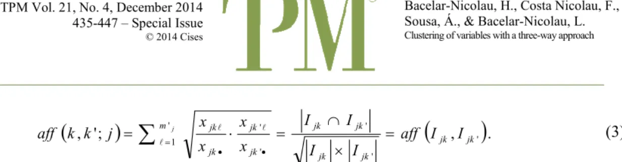
. ' ' ' ' 1 ' ' jk jk jk jk jk jk m jk jk jk jk I I aff I I I I x x x x j k k aff j = × ∩ = ⋅ =

∑

₌ • • l l l (3)

Consequently, for interval data the local affinity between a pair

(

k

, k

'

)

of intervals is also a

generalized Ochiai coefficient, which might be computed either from formula (3) or from the gen-eralized 2 × 2 contingency Table 4, associated with the pair

(

k

, k

'

)

of interval variables over the j-th

group. Instead of the usual cardinals in a 2 × 2 contingency table associated to a pair of binary vari-ables, agreements or disagreements for a pair of intervals are measured by the respective interval ranges, in Table 3. Here, Ic_jk represents the complementary interval of Ijk in the domain Ij.

TABLE 4

Table of agreements and disagreements for a pair

(

k

, k

'

)

of interval variables

k\k' Agreement Disagreement Total

Agreement s_j= I_jk∩I_jk' c jk jk j I I u = ∩ _' sj+uj = Ijk Disagreement c _jk' jk j I I v = ∩ c jk c jk j I I t = ∩ _' vj+tj = Icjk Total sj+vj = Ijk' c ' jk j j t I u + = I j

Asymptotic Permutation Standardized Affinity Coefficient

Using prior knowledge as a reference hypothesis may allow us to compute asymptotic standardized affinity values and the corresponding cumulative distribution function values, giv-ing place to new similarity coefficients and to new probabilistic clustergiv-ing models (PCM), instead of empirical clustering models. A reference hypothesis usually stands in this probabilistic ap-proach not only as a convenient reference point, but also has a natural interpretation, depending on the type of data and context.

In a three-way clustering probabilistic analysis, the random variable aff(k,k';j) has an as-ymptotic normal distribution, and under a permutation reference hypothesis based on the limit theorem of Wald and Wolfowitz (1944), the asymptotic mean value and variance are as follows (Kendall & Stuart, 1967):

(

)

_∑

_∑

= • = • = µ j j m jk jk m jk jk j * WW x x x x m j k k 1 ' ' ' ' 1 1 ; ' , l l l l

(

)

. x x m x x x x m x x m j k k j j j j m m jk jk j jk jk m m jk jk j jk jk j * WW 2 1 '1 ' ' ' ' ' 2 1 '1 ' 2 1 1 1 1 ; ' ,

∑

∑

∑

∑

= • = • = • = •         − ×         − − = σ l l l l l l l l

Thus the generalized affinity coefficient a(k,k')between variables k, k' ∈ V gives place to (for interval variables use m'j instead of mj as explained in the above section concerning the

(

)

(

)

_∑

(

)

= π = = n j * WW j * WW k k a k k .aff k k j a 1 ; ' , ' , ' , ,

whereaff

(

k k j

)

[

aff

(

k k j

)

(

k k j

)

]

/ *WW

(

k k j

)

* WW * WW , '; , '; , '; , '; 2 σ µ − = .

Then, a probabilistic coefficient α_WW

(

k, k'

)

between two variables k, k' ∈ V, is as follows:

(

k,k'

)

P

[

A

(

k,k'

)

a

(

k,k'

)

]

ˆ

(

k,k'

)

[

a*

(

k,k'

)

]

WW * * WW WW = ≤ ≅α =Φ α

where Φ denotes the cumulative distribution function of the standard normal distribution and A*

represents an asymptotic standardized random variable. Applications to simulated data (Sousa, 2005) assure that convergence to the normal distribution is quite fast (n > 10 in most cases). A large value of the probabilistic coefficient means that the observed affinity value is significantly larger than one might expect, under the reference hypothesis. Therefore this probabilistic coeffi-cient validates the affinity coefficoeffi-cient between twovariables k, k' in a probabilistic scale (e.g., H. Bacelar-Nicolau, 1988, 2000; H. Bacelar-Nicolau et al., 2010; Lerman, 1972, 1981, 2000; Nico-lau & H. Bacelar-NicoNico-lau, 1982, 1998). Thus α_WW

(

k ,k'

)

is sometimes called Validity Link (VL) similarity coefficient.

Several good proprieties of the generalized affinity coefficient between (homogenous or heterogeneous) variables, as well as of the corresponding standard and probabilistic coefficients have so far been demonstrated and several applications to simulated or to real data have been analyzed. In this perspective an adaptive/parametric formula, such as Nicolau and H. Bacelar-Nicolau’s extension of the Lance and Williams (1967) adaptive formula to VL similarity coeffi-cients (e.g., H. Bacelar-Nicolau, 1988, 2002; Lerman, 1981; Nicolau & H. Bacelar-Nicolau, 1998) generates new aggregation criteria and allows us to compare probabilistic or semi-probabilistic cluster-ing models in an easy way.

A PCM or a semi-PCM operates in an exploratory framework where prior knowledge about the data structure may be used as a complementary tool to extract knowledge from its clus-tering hierarchical structure. Comparisons of such models have so far been developed mainly in-side some adaptive families, based on a suitable set of parameter values. Other methods are being studied. In the present work we use an adaptive family depending on two real valued parameters ε, ξ

∈

[0,1], so that the single linkage criterion corresponds to (ε = 1, ξ = 0), while AVL and AVB aggregation methods are obtained with respectively (ε = 1, ξ = 1) and (ε = 1, ξ = 0.5). This is illustrated in the case study of the following section. By varying ξ from 0 to 1, with ε = 1, one may for instance analyze how the VL models evolve, when going from the chaining effect asso-ciated to the first criterion, toward the symmetry/equicardinality effect assoasso-ciated to AVL (e.g., H. Bacelar-Nicolau, 1988, 2002; Lerman, 1981; Nicolau & H. Bacelar-Nicolau, 1998).

CASE STUDY

The data resulted from the application of the Parenting Stress Index (PSI; Abidin, 1997) to measure stress in parent-child relationships on a sample of three groups of parents: parents of children with attention deficit/hyperactivity disorder, parents of children with asthma and a con-trol group of parents of children with neither diagnosis of deficit/hyperactivity disorder, nor asthma (Magalhães, 2005; Nicolau et al., 2007). These data have been used as an illustrative example in several statistical studies.

This research concerns 13 scales of the PSI and the corresponding scale scores (sum of Likert scale item values), identifying sources of stress within the family. Regarding children there are six scales: Distractibility/Hyperactivity (E1); Reinforcement of Parent (E2); Mood (E3); Accept-ability (E4); AdaptAccept-ability (E5); Demandingness (E6). Concerning parents there are seven scales: Competence (E7); Attachment (E8); Role Restriction (E9); Depression (E10); Spouse (E11); Isola-tion (E12); Health (E13).

The purpose here is to obtain a typology of the 13 scales, that is to search for a classifica-tion of variables, described by the three groups of parents. Each group had initially 30 respondents, but a missing values analysis detected 13 response patterns with missing values: five in the first group, six in the second group, and two in the third group, corresponding to a total sample of 77 respondents without missing values. All the children are between 6 and 10 years old.

Using Generalized Three-Way Affinity Coefficient

The three groups analyzed contained respectively 25 (Group 1), 24 (Group 2), 28 (Group 3) respondents respectively corresponding to a total sample of 77 individuals. Hierarchical cluster analysis was applied to classify the 13 PSI scales, using the empirical and probabilistic affinity coefficients described above in the sections titled “Generalized three-way affinity coefficient” and “Asymptotic permutation standardized affinity coefficient” with parents groups Gj (j = 1,2,3),

variables/scales Vk (k = 1,...,13), rows (ℓ = 1,..., mj) of each j-th sub-table so that m1 = 25, m2 =

24, m3 = 28, and πj = 1/3 (j = 1,2,3). In this work only results obtained from the probabilistic

co-efficient are referred to, together with four aggregation criteria: Single link (SL), Complete link (CL), and two probabilistic criteria, AVB and AVL. Thus obtaining two semi-PCM and two PCM. Aggregation criteria SL, AVB, and AVL belong to the same adaptive family.

The hierarchical trees or dendrograms obtained are represented below (Figure 1). Several quality statistics, which are not included here, were used for each clustering model helping for instance to choose the most significant partitions of clusters.

The four hierarchical clustering trees present several common clusters, mostly merging in the same way, especially in the CL, AVB, and AVL cases. Considering the three aggregation cri-teria belonging to the parametric family referred to above, we may easily observe how the den-drograms progress when going from SL (ε = 1, ξ = 0) to AVL (ε = 1, ξ = 1) through AVB (ε = 1, ξ = 0.5) methods. This is also supported by the usual tables of quality statistics associated to each clustering model and computed by the statistical software. Here we mention some of these parti-tions without giving the corresponding tables of values. In summary we may observe that: – the following pairs of scales are common to all models: {E2 (Reinforcement of Parent), E3 (Mood)}; {E5 (Adaptability), E7 (Competence)}; {E9 (Role Restriction), E11 (Spouse)}; {E12 (Isolation), E13 (Health)};

– in all models, cluster {E9, E11} joins {E4 (Acceptability)};

– in the three CL, AVB, and AVL models, cluster {E12, E13} joins {E8 (Attachment)}. In the SL case they are quite near, but the chain effect is already working;

– in the three models CL, AVB, and AVL clusters {E2, E3} and {E12, E13, E8} merge together at the 10-th level of the dendrogram, corresponding to the maximum value of the quality statistics,

FIGURE 1

Dendrograms issued from original data, two empirical and two probabilistic aggregation criteria.

that is to the best classification. At this level, AVB and AVL methods propose the same classification in three clusters: the previous one, the small-strong cluster {E5, E7} and the cluster joining {E9, E11} and {E4 (Acceptability)} to {E1 (Distractibility/Hyperactivity), E6 (Demandingness), E10 (Depression)}; – at 11-th level all three CL, AVB, and AVL models give the second most significant partition in the same two clusters of scales.

We do not go into a psychological interpretation in this paper. We just point out one of the first features that appear to be appealing to both statisticians and psychologists for future de-velopments: using the generalized affinity coefficient and its probabilistic coefficient re-enforces the tendency to join sources of stress concerning children with sources concerning parents them-selves at lower levels of the dendrograms.

Using Three-Way Affinity Coefficient with Interval-Type Variables

Instead of basing our study on incomplete sub-samples, because of the presence of miss-ing data, the interval approach as described in the section above entitled “Application of

three-CL Dendrogram SL Dendrogram (ε = 1, ξ = 0)

way affinity coefficient to interval-type variables” allows us to use the complete groups. Thus each group Gj (j = 1,…,3) refers to the total sub-sample, with m_j = 30 (j = 1,…,3), and is

de-scribed over each variable Vk (k = 1,...,13) by an interval of the real axis: lower and upper limits

are respectively the minimum and maximum values that Gj takes over Vk. An alternative

ap-proach could consist in replacing missing values by medians or by other convenient values (e.g., Silva et al., 2002). The intervals approach here is a different way to deal with missing values in a whole study based on the affinity coefficient and its robustness properties.

According to expressions (2) and (3) we may compute the generalized three-way affinity coefficient between interval variables by choosing two different ways of computing the local af-finities, which correspond respectively to the first left part of formula (2), that is using a unique algorithm either Vk is or not an interval variable ― an interesting approach for instance when

dif-ferent types of variables are involved ― or to its right part using the generalized Ochiai coeffi-cient for interval variables.

Again only clustering models based on the probabilistic coefficient and the four aggrega-tion criteria as used in the previous secaggrega-tion concerned with the generalizaaggrega-tion of the three-way affinity coefficient, are referred to in this section. Also the same quality statistics were applied. The dendrograms obtained are represented below (Figure 2).

FIGURE 2

Dendrograms issued from interval data, two empirical and two probabilistic aggregation criteria. CL Dendrogram

SL Dendrogram (ε = 1, ξ = 0)

It can be seen that although data representations using either the original (incomplete) data matrix or the transformed one based on the intervals approach seem quite different (see Ta-bles 1 and 3), both groups of four clustering models kept the most important features of cluster-ing structure in a similar way.

Concerning graphical representations, excepting SL dendrograms (first top dendrograms in Figures 1 and 2), which show the usual chain effect, at 11-th level all three CL, AVB, and AVL models give the same second most significant partition in two clusters of scales, in both ap-proaches. The larger upper cluster presents a few natural differences from the one obtained with the first approach, while the bottom cluster represents a consistent group identically built in both approaches and by all three CL, AVB, and AVL models.

CONCLUSIONS

In this work we refer to empirical and probabilistic hierarchical clustering models of variables based on the generalized affinity coefficient for three-way (also called symbolic) data. The particular case of interval type variables is analyzed and used as an alternative method in the case of missing data. Some information is lost when dealing with intervals instead of the original values, but we gain in robustness of the results and by the fact that the whole sample can be ana-lyzed. Moreover pairs of interval variables may also be directly analyzed in the same way that pairs of binary variables usually are. From a (generalized) 2 × 2 contingency table, instead of cardinals (for binary data), cells contain ranges of appropriate intervals. We briefly discuss a case-study (which has been used as an illustrative example in other applied researches), where aggregation criteria come from an adaptive family of semi-probabilistic and probabilistic meth-ods. As might be expected in this case, results on hierarchical clustering of original and of inter-val variables are not very different and often the second ones gain in quality of typology explana-tion. Obviously, the three-way approach partially described here has increasing relevance when larger data bases are used, mostly in a data mining context.

ACKNOWLEDGEMENTS

This research was partially supported by ISAMB (Faculty of Medicine, University of Lisbon, Lisbon) and

CEEAplA (University of the Azores, Ponta Delgada, Azores).

REFERENCES

Abidin, R. R. (1997). Parenting Stress Index: A measure of the parent-child system. In C. P. Zalaquett & R. J. Wood (Eds.), Evaluating stress: A book of resources (pp. 277-291). Lanham, MD: Scarecrow Education.

Bacelar-Nicolau, H. (1985). The affinity coefficient in cluster analysis. In M. J. Beckmann, K.-W. Gaede, K. Ritter, & H. Schneeweiss (Eds.), Methods of operations research (Vol. 53, pp. 507-512). Munchen, Germany: Verlag Anton Hain.

Bacelar-Nicolau, H. (1988). Two probabilistic models for classification of variables in frequency tables. In H.-H. Bock (Ed.), Classification and related methods of data analysis (pp. 181-186). North Hol-land: Elsevier Sciences Publishers B.V.

Bacelar-Nicolau, H. (2000). The affinity coefficient. In H.-H. Bock & E. Diday (Eds.), Analysis of

sym-bolic data: Exploratory methods for extracting statistical information from complex data. Series:

Studies in classification, data analysis, and knowledge organization (pp. 160-165). Berlin-Heidelberg,

Germany: Springer-Verlag.

Bacelar-Nicolau, H. (2002). On the generalized affinity coefficient for complex data. Byocybernetics and

Biomedical Engineering, 22, 31-42.

Bacelar-Nicolau, H., Nicolau, F. C., Sousa, Á., & Bacelar-Nicolau, L. (2009). Measuring similarity of complex and heterogeneous data in clustering of large data sets. Biocybernetics and Biomedical

En-gineering, 29, 9-18.

Bacelar-Nicolau, H., Nicolau, F. C., Sousa, Á., & Bacelar-Nicolau, L. (2010). Clustering complex

Hetero-geneous data using a probabilistic approach. Proceedings of Stochastic Modeling Techniques and

Data Analysis International Conference (SMTDA2010), 85-93. Retrieved from http://www. smtda. net/images/SMTDA_2010_Proceedings_pp_1-356.pdf

Bacelar-Nicolau, L. (2002). Caracterização dos sistemas de informação das organizações com base no

modelo de olan. Aplicação de modelos de classificação hierárquica aos organismos da

Administração Pública [Characterization of information systems from organizations based on the

Nolan model. Application of hierarchical classification models to Public Administration Agencies]. (Unpublished master’s thesis). ISEGI, New University of Lisbon, Portugal.

Bock, H.-H., & Diday, E. (Eds.). (2000). Analysis of symbolic data: Exploratory methods for extracting

statistical information from complex data. Series: Studies in classification, data analysis, and

knowl-edge organization. Berlin-Heidelberg, Germany: Springer-Verlag.

Domenges, D., & Volle, M. (1979). Analyse factorielle sphérique: Une exploration [Spherical factor analy-sis: An exploration]. Annales de l’I SEE, 35, 3-84.

Kendall, M. G., & Stuart, A. (1967). The advanced theory of statistics (Vol. 2). London, England: Griffin. Lance, G. N., & Williams, W. T. (1967). A general theory of classificatory sorting strategies. Hierarchical

systems. The Computer Journal, 9, 373-380. doi:10.1093/comjnl/9.4.373

Lerman, I. C. (1973). Étude distributionnelle de statistiques de proximité entre structures algébriques finies du même type; application à la classification automatique [Statistical distribution of proximity measures between combinatorial structures. Application to cluster analysis].Cahiers du Bureau

universitaire de recherche opérationnelle: Vol. 19 (Série Recherche). Paris, France: Institut de

statistique des universités de Paris.

Lerman, I. C. (1981). Classification et analyse ordinale des données [Data classification and ordinal analy-sis].Paris, France: Dunod.

Lerman, I. C. (2000). Comparing taxonomy data. Revue Mathématiques et Sciences Humaines, 38, 37-51. Magalhães, B. (2005). Stress parental e idade escolar: Contributo para a compreensão dos factores de

stress em três grupos de famílias [Parental stress and school age: Contribution for understanding stress

factors in three groups of families]. (Unpublished master’s thesis). University of Lisbon, Portugal. Matusita, K. (1951). On the theory of statistical decision functions. Annals of the Institute of Statistical

Mathemathics, 3, 17-35. doi:10.1007/BF02949773

Matusita, K. (1955). Decision rules, based on distance for problems of fit, two samples and estimation.

An-nals of the Institute of Statistical Mathemathics, 26, 631-640.

Nicolau, F. C., & Bacelar-Nicolau, H. (1982). ouvelles méthodes d’agrégation basées sur la fonction de

répartition [New aggregation methods based on the probabilistic distribution function]. Collection

Séminaires INRIA, Classification Automatique et Perception par Ordinateur, 45-60.

Nicolau, F. C., & Bacelar-Nicolau, H. (1998). Some trends in the classification of variables. In E. C. Hayashi, K. Yajima, H.-H. Bock, N. Oshumi, Y. Tanaka, & Y. Baba (Eds.), Data science,

classification and related methods. Series: Studies in classification, data analysis, and knowledge

organization (pp. 89-98). Berlin-Heidelberg, Germany: Springer-Verlag.

Nicolau, F. C., Bacelar-Nicolau, H., Sousa, Á., Bacelar-Nicolau, L., Silva, O., & Magalhães B. (2007).

Probabilistic models in three way cluster analysis. Proceedings of the 56th Session of the

Interna-tional Statistical Institute, LXII, 1861-1866. Retrieved from http://isi.cbs.nl/iamamember/CD7-Lisboa2007/Bulletin-of-the-ISI-Volume-LXII-2007.pdf

Nikulin, M. S. (2001). “Hellinger distance”. In M. Hazewinkel (Ed.), Encyclopedia of mathematics. Berlin-Heidelberg, Germany: Springer-Verlag. ISBN 978-1-55608-010-4

Ochiai, A. (1957). Zoogeographical studies on the soleoid fishes found Japan and its neighboring regions.

Bulletin of the Japanese Society, 22, 526-530.

Silva, A. L., Bacelar-Nicolau, H., & Saporta, G. (2002). Missing data in hierarchical classification of vari-ables. A simulation study. In K. Jajuga, A. Sokołowski, & H.-H. Bock (Eds.), Classification,

cluster-ing, and data analysis ― Recent advances and applications. Series: Studies in classification, data

analysis, and knowledge organization (pp. 121-128). Berlin-Heidelberg, Germany: Springer-Verlag.

Silva, A. L., Saporta, G., & Bacelar-Nicolau, H. (2004). Missing data and imputation methods in partition of variables. In D. Banks, F. R. McMorris, P. Arabie, & W. Gaul (Eds.), Classification, clustering,

and data mining applications. Series: Studies in classification, data analysis, and knowledge

Sousa, Á. (2005). Contribuições à Metodologia VL e índices de validação para Dados de atureza Complexa [Contributions to the VL methodology and validation indexes for complex data]. (Unpublished PhD thesis). University of Azores, Portugal.

Sousa, Á., Nicolau, F. C., Bacelar-Nicolau, H., & Silva, O. (2010). Weighted generalized affinity coeffi-cient in cluster analysis of complex data of the interval type. Biometrical Letters, 47, 45-56.

Sousa, Á., Tomás, L., Silva, O., & Bacelar-Nicolau, H. (2013). Symbolic data analysis for the assessment of user satisfaction: An application to reading rooms services. European Sientific Journal, 3(Special Edition), 39-48.

Souza, R. M. C. R., & De Carvalho, F. A. T. (2004). Clustering of interval data based on City-Block dis-tances. Pattern Recognition Letters, 25, 353-365. doi:10.1016/j.patrec.2003.10.016

Wald, A., & Wolfowitz, J. (1944). Statistical test based on permutations of the observations. Annals of