A HYBRID MULTI-OBJECTIVE BAYESIAN ESTIMATION OF DISTRIBUTION ALGORITHM THESIS

(1)

ENGINEERING

MARCELLA SCOCZYNSKI RIBEIRO MARTINS

A HYBRID MULTI-OBJECTIVE BAYESIAN ESTIMATION OF

DISTRIBUTION ALGORITHM

THESIS

(2)

A HYBRID MULTI-OBJECTIVE BAYESIAN ESTIMATION OF

DISTRIBUTION ALGORITHM

Thesis submitted to the Graduate Program in Electrical and Computer Engineering of Federal University of Technology - Paraná in partial fulfillment for the degree of “Doutor em Ciências” (Computer Engineering).

Advisor: Myriam Regattieri Delgado

Co-Advisor: Ricardo Lüders

(3)

Martins, Marcella Scoczynski Ribeiro

N244h A hybrid multi-objective bayesian estimation of distribution 2017 algorithm / Marcella Scoczynski Ribeiro Martins.-- 2017.

124 f. : il. ; 30 cm

Texto em inglês com resumo em português Disponível também via World Wide Web

Tese (Doutorado) – Universidade Tecnológica Federal do Pa-raná. Programa de Pós-graduação em Engenharia Elétrica e In-formática Industrial, Curitiba, 2017

Bibliografia: f. 97-108

1. Algoritmos computacionais. 2. Probabilidade (Matemática). 3. Teoria bayesiana de decisão estatística. 4. Algoritmos heurísti-cos. 5. Otimização matemática. 6. Engenharia elétrica – Teses. I. Delgado, Myriam Regattieri de Biase da Silva. II. Lüders, Ricardo. III. Universidade Tecnológica Federal do Paraná. Programa de Pós-Graduação em Engenharia Elétrica e Informática Industrial. IV. Título.

CDD: Ed. 23 – 621.3 Biblioteca Central da UTFPR, Câmpus Curitiba

(4)

Universidade Tecnológica Federal do Paraná Diretoria de Pesquisa e Pós-Graduação

TERMO DE APROVAÇÃO DE TESE Nº 163

A Tese de Doutorado intitulada “A Hybrid Multi-objective Bayesian Estimation of Distribution Algorithm”, defendida em sessão pública pelo(a) candidato(a) Marcella Scoczynski Ribeiro Martins, no dia 11 de dezembro de 2017, foi julgada para a obtenção do título de Doutor em Ciências, área de concentração Engenharia de Computação, e aprovada em sua forma final, pelo Programa de Pós-Graduação em Engenharia Elétrica e Informática Industrial.

BANCA EXAMINADORA:

Prof(a). Dr(a). Myriam Regattieri de Biase da Silva Delgado -Presidente– (UTFPR) Prof(a). Dr(a). Roberto Santana Hermida – (University of the Basque Country) Prof(a). Dr(a). Gilberto ReynosoMeza – (PUC-PR)

Prof(a). Dr(a). Aurora Trinidad Ramirez Pozo – (UFPR) Prof(a). Dr(a). Viviana Cocco Mariani - (PUC-PR)

Prof (a). Dr(a). Lucia Valeria Ramos de Arruda

A via original deste documento encontra-se arquivada na Secretaria do Programa, contendo a assinatura da Coordenação após a entrega da versão corrigida do trabalho.

(5)

As all of these long and hard working years went by, I realize I would not be able to accomplish anything, if God was not by my side. I thank for all the prayers my mother, my family and my friends have said in my behalf. I specially thank my Professors, Myriam and Ricardo, which have always supported me. She is an example of wisdom, kindness and respect - probably she uses a bit of magic too. He does not spare efforts when helping others, and I seek to become a person and a Professor like them, and to have the opportunity to take care of my students like they have done to me: as friends. I would also like to thank Roberto, for the help he has provided for this work. His suggestions and opinions were very important. Plus, I extend my acknowledgment to the Professors who kindly accepted to be part of my presentation board, as well as their important contributions. I also thank Carol, Ledo and Richard, who always pointed out relevant ideas to this research.

I can not forget the great opportunity I had to attend extraordinary conferences due to help of my Graduate Program, the CAPES (Coordenação de Aperfeiçoamento de Pessoal de Nível Superior) government agency, the student grants by ACM (Association for Computing Machinery) and the Department of Electronics - UTFPR Ponta Grossa, where I work. I thank my colleagues Jeferson, Virginia, Claudinor and Frederic, for all the help with classes, laboratories and with the server, where I ran all the experiments.

(6)

invencible. Intentar cuando las fuerzas se desvanecen. Alcanzar la estrella inatingíble; esa es mi búsqueta..."

(7)

MARTINS, Marcella Scoczynski Ribeiro. A HYBRID MULTI-OBJECTIVE BAYESIAN ESTIMATION OF DISTRIBUTION ALGORITHM. 124 f. Thesis – Graduate Program in Electrical and Computer Engineering, Federal University of Technology - Paraná. Curitiba, 2017.

Nowadays, a number of metaheuristics have been developed for dealing with multiobjective optimization problems. Estimation of distribution algorithms (EDAs) are a special class of metaheuristics that explore the decision variable space to construct probabilistic models from promising solutions. The probabilistic model used in EDA captures statistics of decision variables and their interdependencies with the optimization problem. Moreover, the aggregation of local search methods can notably improve the results of multi-objective evolutionary algorithms. Therefore, these hybrid approaches have been jointly applied to multi-objective problems. In this work, a Hybrid Multi-objective Bayesian Estimation of Distribution Algorithm (HMOBEDA), which is based on a Bayesian network, is proposed to multi and many objective scenarios by modeling the joint probability of decision variables, objectives, and configuration parameters of an embedded local search (LS). We tested different versions of HMOBEDA using instances of the multi-objective knapsack problem for two to five and eight objectives. HMOBEDA is also compared with five cutting edge evolutionary algorithms (including a modified version of NSGA-III, for combinatorial optimization) applied to the same knapsack instances, as well to a set of MNK-landscape instances for two, three, five and eight objectives. An analysis of the resulting Bayesian network structures and parameters has also been carried to evaluate the approximated Pareto front from a probabilistic point of view, and also to evaluate how the interactions among variables, objectives and local search parameters are captured by the Bayesian networks. Results show that HMOBEDA outperforms the other approaches. It not only provides the best values for hypervolume, capacity and inverted generational distance indicators in most of the experiments, but it also presents a high diversity solution set close to the estimated Pareto front.

(8)

MARTINS, Marcella Scoczynski Ribeiro. UM ALGORITMO DE ESTIMAÇÃO DE DISTRIBUIÇÃO HÍBRIDO MULTIOBJETIVO COM MODELO PROBABILÍSTICO BAYESIANO. 124 f. Thesis – Graduate Program in Electrical and Computer Engineering, Federal University of Technology - Paraná. Curitiba, 2017.

Atualmente, diversas metaheurísticas têm sido desenvolvidas para tratarem problemas de otimização multiobjetivo. Os Algoritmos de Estimação de Distribuição são uma classe específica de metaheurísticas que exploram o espaço de variáveis de decisão para construir modelos de distribuição de probabilidade a partir das soluções promissoras. O modelo probabilístico destes algoritmos captura estatísticas das variáveis de decisão e suas interdependências com o problema de otimização. Além do modelo probabilístico, a incorporação de métodos de busca local em Algoritmos Evolutivos Multiobjetivo pode melhorar consideravelmente os resultados. Estas duas técnicas têm sido aplicadas em conjunto na resolução de problemas de otimização multiobjetivo. Nesta tese, um algoritmo de estimação de distribuição híbrido, denominado HMOBEDA (Hybrid Multi-objective Bayesian Estimation of Distribution Algorithm ), o qual é baseado em redes bayesianas e busca local é proposto

no contexto de otimização multi e com muitos objetivos a fim de estruturar, no mesmo modelo probabilístico, as variáveis, objetivos e as configurações dos parâmetros da busca local. Diferentes versões do HMOBEDA foram testadas utilizando instâncias do problema da mochila multiobjetivo com dois a cinco e oito objetivos. O HMOBEDA também é comparado com outros cinco métodos evolucionários (incluindo uma versão modificada do NSGA-III, adaptada para otimização combinatória) nas mesmas instâncias do problema da mochila, bem como, em um conjunto de instâncias do modelo MNK-landscape para dois, três, cinco e oito objetivos. As fronteiras de Pareto aproximadas também foram avaliadas utilizando as probabilidades estimadas pelas estruturas das redes resultantes, bem como, foram analisadas as interações entre variáveis, objetivos e parâmetros de busca local a partir da representação da rede bayesiana. Os resultados mostram que a melhor versão do HMOBEDA apresenta um desempenho superior em relação às abordagens comparadas. O algoritmo não só fornece os melhores valores para os indicadores de hipervolume, capacidade e distância invertida geracional, como também apresenta um conjunto de soluções com alta diversidade próximo à fronteira de Pareto estimada.

(9)

–

FIGURE 1 An example of Pareto front and Pareto dominance in the objective space. . 21 –

FIGURE 2 Ilustration of the boundary intersection approach (ZHANG; LI, 2007). . . . 26 –

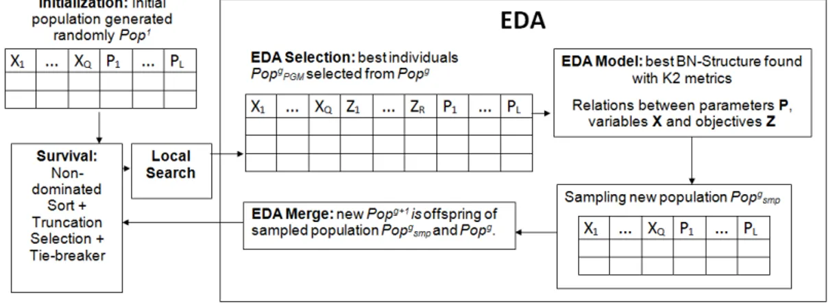
FIGURE 3 The general framework of an EDA. . . 33 –

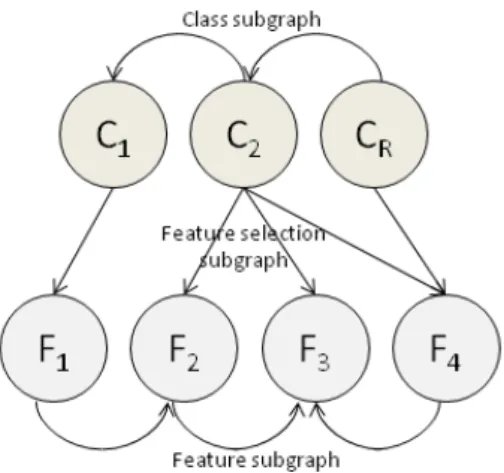
FIGURE 4 An MBN classifier with 3 class variables and 4 feature variables. . . 41 –

FIGURE 5 A naive MBN classifier with 3 class variables and 4 feature variables. . . 43 –

FIGURE 6 The HMOBEDA Framework. . . 55 –

FIGURE 7 An example of the PGM structure used by HMOBEDA. . . 61 –

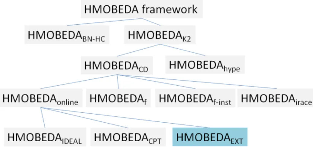
FIGURE 8 Different HMOBEDA versions considered in the experiments. . . 67 –

FIGURE 9 Evidences (blue circles) from the approximated Pareto front with 2 objectives for (a) HMOBEDAIDEAL, (b) HMOBEDAEX T and (c)

HMOBEDACPT. . . 70

–

FIGURE 10 A probabilistic view of the approximated Pareto front for 2 objectives and 100 items for HMOBEDAIDEAL, HMOBEDAEX T and HMOBEDACPT. . . 78

–

FIGURE 11 A probabilistic view of the approximated Pareto front for 2 objectives and 250 items for HMOBEDAIDEAL, HMOBEDAEX T and HMOBEDACPT. . . 78

–

FIGURE 12 The Euclidean distance between each solution and the ideal point for 2 objectives with (a) 100 items and (b) 250 items. . . 79 –

FIGURE 17 For instance 2-100, number of times arc(Z1,Xq)has been captured in the

BN versus a similar measure for arc (Z2,Xq). Each circle corresponds to

one decision variableXq,q∈ {1, . . . ,100}. . . 90

–

FIGURE 18 Glyph representation of the three LS parameters (spokes) for each objective

Z1toZ8of instance 8-100. . . 90

–

FIGURE 19 For M2N20K2 instance, number of times arc(Z1,Xq)has been captured in

the BN versus a similar measure for arc(Z2,Xq). Each circle corresponds

to one decision variableXq,q∈ {1, . . . ,20}. . . 91

–

Z1toZ3of M3N50K6 instance. . . 91

–

Z1toZ8of M8N100K10 instance. . . 92

–

FIGURE 22 An example of structure learned by K2 Algorithm. . . 114 –

(10)

–

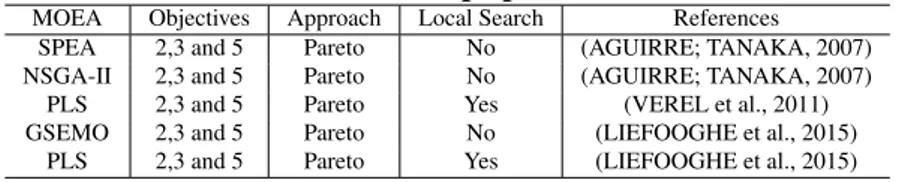
TABLE 1 MOEAs to MOKP main characteristics . . . 49 –

TABLE 2 MOEAs to MNK-landscape problem main characteristics . . . 54 –

TABLE 3 Summarizing EDAs approaches to the knapsack problem and NK-landscape problem . . . 64 –

TABLE 4 HMOBEDAf−inst parameters. . . 69

–

TABLE 5 Parameters of the MOEAs used for solving the MOKP and MNK-landscape problem. . . 70 –

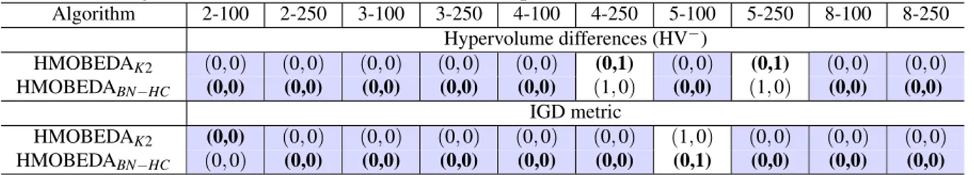
TABLE 6 Results for pairwise comparison between HMOBEDAK2 and

HMOBEDABN−HC using Mann-Whitney-Wilcoxon test with α = 5%

for each problem instance. . . 72 –

TABLE 7 Average Run time (minutes) for each algorithm and instance. . . 73 –

TABLE 8 Results for pairwise run time comparisons between HMOBEDAK2 and

HMOBEDABN−HC using Mann-Whitney-Wilcoxon test with α =5% for

each problem instance. . . 73 –

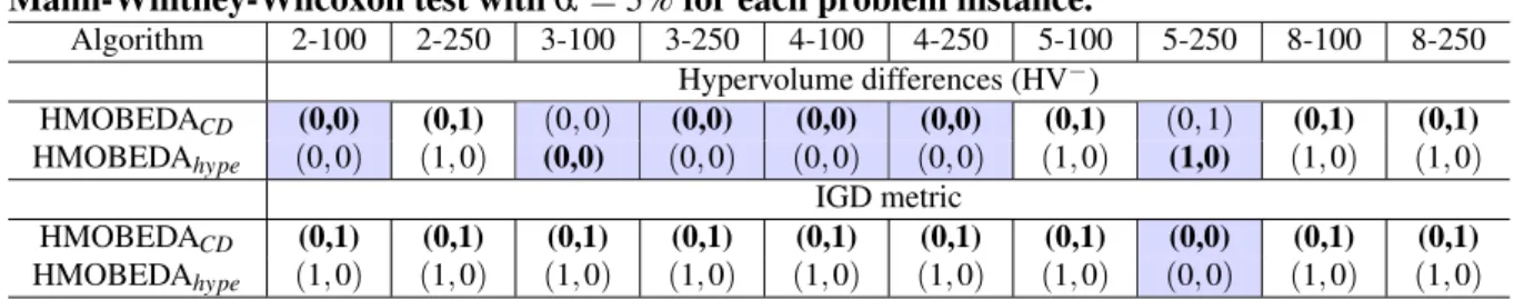
TABLE 9 Results for pairwise comparisons between HMOBEDACD and

HMOBEDAhype using Mann-Whitney-Wilcoxon test with α = 5% for

each problem instance. . . 74 –

TABLE 10 Average run time (minutes) for each algorithm and instance. . . 74 –

TABLE 11 Results for pairwise run time comparisons between HMOBEDACD and

HMOBEDAhype using Mann-Whitney-Wilcoxon test with α =5% for each

problem instance. . . 74 –

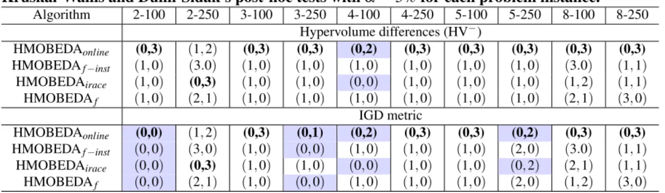
TABLE 12 Results for pairwise comparisons between HMOBEDAonline and its off-line

versions using Kruskal-Wallis and Dunn-Sidak’s post-hoc tests withα=5% for each problem instance. . . 75 –

TABLE 14 Results for pairwise run time comparisons among HMOBEDAonline and the

off-line versions using Kruskal-Wallis and Dunn-Sidak’s post-hoc tests with α=5% for each problem instance. . . 75 –

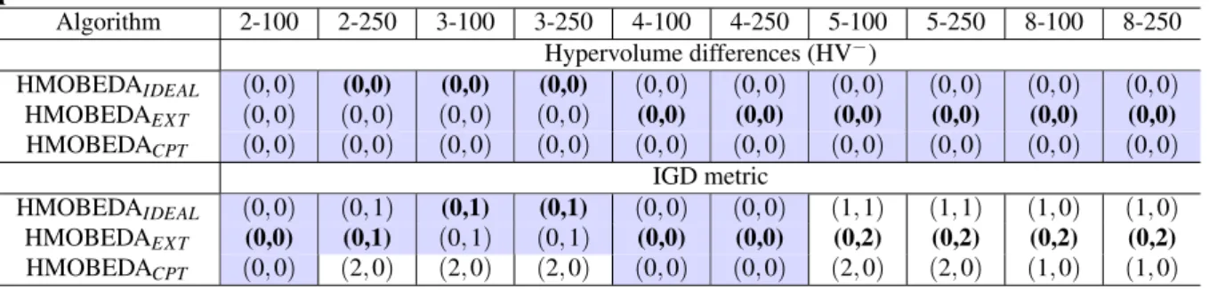
TABLE 15 Results for pairwise comparisons between HMOBEDAIDEAL,

HMOBEDAEX T and HMOBEDACPT using Kruskal-Wallis and

Dunn-Sidak’s post-hoc tests withα=5% for each problem instance. . . 76 –

TABLE 17 Results for pairwise run time comparisons between HMOBEDAIDEAL,

HMOBEDACPT and HMOBEDAEX T versions using Kruskal-Wallis and

Dunn-Sidak’s post-hoc tests withα=5% for each problem instance. . . 77 –

TABLE 18 Average HV− _{and IGD over 30 executions. . . 82} –

TABLE 19 Capacity metrics over 30 executions for each algorithm. The best values are in bold . . . 82 –

TABLE 20 Average Run time (minutes) for each algorithm and instance. . . 83 –

TABLE 21 Average HV− _{over 30 independent executions. . . 84} –

(11)

–

TABLE 24 Error Ratio over 30 executions for each algorithm. The best values are in bold. . . 87 –

(12)

–

ALGORITHM 1 K2 Algorithm . . . 42 –

ALGORITHM 2 BN-HC Algorithm . . . 43 –

ALGORITHM 3 HMOBEDA Framework . . . 57 –

ALGORITHM 4 Local Search (LS) . . . 59 –

ALGORITHM 5 Bit-flip Neighborhood . . . 60 –

ALGORITHM 6 Set Neighborhood . . . 60 –

ALGORITHM 7 NSGA-II . . . 116 –

ALGORITHM 8 NSGA-III . . . 119 –

(13)

AffEDA Affinity Propagation EDA ALS Adaptive Local Search BI Boundary Intersection BKP Bounded Knapsack Problem

BMDA Bivariate Marginal Distribution Algorithm

BMOA Bayesian Multi-objective Optimization Algorithm

BN Bayesian Network

BN-HC Bayesian Network Greedy Hill Climber Algorithm BOA Bayesian Optimization Algorithm

CD Crowding Distance

GA Genetic Algorithm

cGA Compact Genetic Algorithm

COMIT Combining Optimizer with Mutual Information Tree DAG Directed Acyclic Graph

DR Dominance Rank

EA Evolutionary Algorithm

ER Error Ratio

EBNA Estimation of Bayesian Network Algorithm ECGA Extended Compact Genetic Algorithm EDA Estimation of Distribution Algorithm FDA Factorized Distribution Algorithm

GRASP Greedy Randomized Adaptive Search Procedure hBOA Hierarchical Bayesian Optimization Algorithm

HC Hill Climbing

HMEA Hybrid Multi-objective Evolutionary Algorithm

HMOBEDA Hybrid Multi-objective Bayesian Estimation of Distribution Algorithms HypE Fast Hypervolume-based Many-objective Optimization

IBMOLS Iterated Local Search based on R2 Quality Indicator IGD Inverted Generational Distance

ILS Iterated Local Search

IMMOGLS Ishibuchi’s and Murata’s Multiple-objective Genetic Local Search MaOP Many Objective Optimization Problem

MBN Multidimensional Bayesian Network

MIMIC Mutual Information Maximization for Input Clustering MLE Maximum Likelihood Estimate

MNK Multi-objective NK

MOA Markovianity-based Optimization Algorithm

MOEA/D Multi-objective Evolutionary Algorithm Based on Decomposition MOEA Multi-objective Evolutionary Algorithm

(14)

MoMad Memetic Algorithm for Combinatorial Multi-objective MOP Multi-objective Optimization Problem

M-PAES Memetic-Pareto Archive Evolution Strategy NPGA Niched Pareto Genetic Algorithm

NSGA Non-dominated Sorting in Genetic Algorithm ONVG Overall Non-dominated Vector Generation PBIL Population-based Incremental Learning PESA Pareto Envelope-Based Selection Algorithm PGM Probabilistic Graphical Model

PLS Pareto Local Search pmf probability mass function

S-MOGLS Simple Multi-Objective Genetic Local Search Algorithm SMS-EMOA Multi-objective selection based on dominated hypervolume SPEA Strength Pareto Evolutionary Algorithm

TTP Travelling Thief Problem

(15)

AP Approximated Pareto-front

arq Profit of itemq=1, . . . ,Q, according to knapsackr=1, . . . ,R

brq Weight of itemqaccording to knapsackr

B Set of binary numbers

cr Constraint capacity of knapsackr

f(x) Mono-objective function

E(θ_{m jk}|Nm j,B) Expected value ofθm jkgiven Bayesian Estimate

λ λ

λ Non-negative weight vector

Maxeval Maximum number of solutions evaluation

N Population size

Nbest Maximum of parents selected to provide the offspring population

Niter Maximum number of iterations of the considered local search

Nls Total number of neighbors

Nm j Number of individuals inPopwith the parents ofYmare instantiated to its j-th

combination

Nm jk Number of observations for whichYm assumes the k-th value given the j-th

combination of values from its parents

NPGM Number of selected individuals to composePopPGM

ND Set of non-dominated solutions in the variable space

p Vector of elements associated with the local search parameters

Pls Probability of occurrence of Local Search

Popg Population of generationg

Popg_merged Joint of current population and offspring population

Popg_best Population of selected individuals from generationg PopI Population of improved individuals

Popg_{o f f spring} Population generated by genetic operations

PopPGM Population ofNPGM individuals to support the PGM

Popsmp Population of Sampled individuals

Q Decision variable vector dimension

R Number of objectives

Re f Reference front

R Real numbers set

ˆ

θm jk Maximum Likelihood Estimate parameter forθm jk

TFnbh Function type used by local search to compute the neighbor fitness

Tnbh Local Search neighborhood type: drop-add (DAd) or insert(Ins)

TotF Total number of Pareto fronts

x Decision variable vector

X Decision variable space

z Vector of objective functions

(16)

(17)

1 INTRODUCTION . . . 13

1.1 OBJECTIVES . . . 15

1.2 CONTRIBUTIONS . . . 15

1.3 ORGANIZATION . . . 19

2 MULTI-OBJECTIVE OPTIMIZATION . . . 20

2.1 BASIC CONCEPTS . . . 20

2.2 PARETO DOMINANCE-BASED APPROACHES . . . 22

2.3 SCALARIZING FUNCTION-BASED METHODS AND OTHERS APPROACHES 23 2.3.1 Weighted Sum approach . . . 24

2.3.2 Tchebycheff approach . . . 25

2.3.3 Boundary Intersection approach . . . 25

2.4 SOLUTION QUALITY INDICATORS . . . 26

2.4.1 Hypervolume Indicator - HV . . . 30

2.4.2 Inverted Generational Distance - IGD . . . 30

2.4.3 Capacity metrics . . . 30

2.5 SUMMARY . . . 31

3 ESTIMATION OF DISTRIBUTION ALGORITHM - EDA . . . 32

3.1 BASIC CONCEPTS . . . 33

3.2 CLASSIFICATION . . . 34

3.3 BAYESIAN NETWORK . . . 35

3.3.1 Basic concepts . . . 35

3.3.2 Parameter estimation . . . 36

3.3.3 Structure . . . 39

3.3.4 Naive BN . . . 40

3.4 SUMMARY . . . 44

4 THE MULTI-OBJECTIVE PROBLEMS ADDRESSED IN THIS WORK . . . 45

4.1 THE MULTI-OBJECTIVE KNAPSACK PROBLEM . . . 45

4.1.1 General formulation . . . 45

4.1.2 MOEA to solve MOKP . . . 47

4.1.3 EDA approaches for MOKP . . . 49

4.2 THE MULTI-OBJECTIVE NK-LANDSCAPE PROBLEM . . . 51

4.2.1 General formulation . . . 51

4.2.2 MOEA approaches for MNK-landscape . . . 53

4.3 SUMMARY . . . 54

5 HYBRID MULTI-OBJECTIVE BAYESIAN ESTIMATION OF DISTRIBUTION ALGORITHM . . . 55

5.1 GENERAL SCHEME . . . 55

5.2 SOLUTION ENCODING . . . 56

5.3 HMOBEDA FRAMEWORK . . . 57

5.3.1 Initialization . . . 58

(18)

5.3.4 Probabilistic model . . . 60

5.4 DIFFERENCES FROM THE LITERATURE . . . 62

5.5 SUMMARY . . . 64

6 EXPERIMENTS AND RESULTS . . . 65

6.1 SETUP OF EXPERIMENTS . . . 66

6.1.1 Problem instances . . . 66

6.1.2 HMOBEDA alternative versions . . . 66

6.1.3 Cutting edge evolutionary approaches from the literature . . . 70

6.2 RESULTS . . . 71

6.2.1 Comparing alternative versions of HMOBEDA . . . 72

6.2.1.1 BN Structure Estimation: HMOBEDAK2x HMOBEDABN−HC . . . 72

6.2.1.2 Tie-breaker criterion: HMOBEDACDx HMOBEDAhype . . . 73

6.2.1.3 LS parameter tuning: Online x Off-line versions . . . 74

6.2.1.4 Setting evidence: HMOBEDAIDEALx HMOBEDAEX T x HMOBEDACPT . . . 76

6.2.2 Comparing HMOBEDAEX T with cutting edge approaches . . . 81

6.2.2.1 Experiments with MOKP . . . 82

6.2.2.2 Experiments with MNK-landscape problem . . . 83

6.2.3 Analyzing the Probabilistic Graphic Model . . . 88

6.3 SUMMARY . . . 92

7 CONCLUSION . . . 94

7.1 FUTURE WORK . . . 95

REFERENCES . . . 97

Appendix A -- EXAMPLE OF THE K2 ALGORITHM . . . 109

Appendix B -- CUTTING EDGE EVOLUTIONARY ALGORITHMS . . . 115

B.1 NSGA-II . . . 115

B.2 S-MOGLS . . . 117

B.2.1 S-MOGLS Local Search Procedure . . . 117

B.3 NSGA-III . . . 118

B.4 MBN-EDA . . . 121

(19)

1 INTRODUCTION

In many optimization problems, maximizing/minimizing two or more objective functions represents a challenge to a large number of optimizers (LUQUE, 2015). This class of problems is known as Multi-objective Optimization Problems (MOP), and solving MOPs has thus been established as an important field of research (DEB, 2001). In the past few years, problems with more than three objectives are becoming usual. They are referred as Many Objective Optimization Problems (MaOP) (ISHIBUCHI et al., 2008).

MOPs and specially MaOPs contain several, usually conflicting, objectives. This means, optimizing one objective does not necessarily optimize the others. Due to the objectives trade-off, a set called Pareto-optimal is generated at the decision variable space. Different approaches have been proposed to approximate the Pareto-optimal front (i.e. Pareto-optimal corresponding objectives) in the objective space in various scenarios (DEB, 2001).

Evolutionary Algorithms (EA) and other population-based metaheuristics have been widely used for solving multi and many objective optimization, mainly due to their ability to find multiple solutions in parallel and to handle the complex features of such problems (COELLO, 1999). For combinatorial optimization, local optimizers can also be aggregated to capture and exploit the potential regularities that arise in the promising solutions.

Several Multi-objective Evolutionary Algorithms (MOEA) incorporating local search (LS) have been investigated, and these hybrid approaches can often achieve good performance for many problems (LARA et al., 2010; ZHOU et al., 2011, 2015). However, as discussed in Martins et al. (2016) and Martins et al. (2017a), they still present challenges, such as the choice of suitable LS parameters e.g., the type, frequency and intensity of LS applied to a particular candidate solution.

(20)

is necessary when setting these two parameters. Moreover, when only a subset of individuals undergo local optimization, their choice becomes an issue. Finally, the type of LS favors different neighborhood structures. All these parameters affect the algorithm’s performance making auto-adaptation an important topic for Hybrid EAs and MOEAs.

Another strategy widely used in evolutionary optimization is the probabilistic modeling, which is the basis of an Estimation of Distribution Algorithm (EDA) (MÜHLENBEIN; PAAB, 1996). The main idea of EDAs (LARRAÑAGA; LOZANO, 2002) is to extract and represent, using a probabilistic model, the regularities shared by a subset of high-valued problem solutions. New solutions are then sampled from the probabilistic model guiding the search toward areas where optimal solutions are more likely to be found. Normally, a Multi-objective Estimation of Distribution Algorithm (MOEDA) (KARSHENAS et al., 2014) integrates both model building and sampling techniques into evolutionary multi-objective optimizers using special selection schemes (LAUMANNS; OCENASEK, 2002). A promising probabilistic model, called Probabilistic Graphical Model (PGM) that combines graph and probability theory, has been adopted to improve EDAs and MOEDAs performance (LARRAÑAGA et al., 2012). Most of MOEDAs developed to deal with combinatorial MOPs adopt Bayesian Networks as their PGM.

In this work, we propose a different approach called Hybrid Multi-objective Bayesian Estimation of Distribution Algorithm (HMOBEDA) based on a joint probabilistic modeling of decision variables, objectives, and parameters of a local optimizer. Some recent MOEDA-based approaches model a joint distribution of variables and objectives in order to explore their relationship, which means investigating how objectives influence variables and vice versa. However, our approach also includes an LS parameter tuning in the same model. The rationale of HMOBEDA is that the embedded PGM can be structured to sample appropriate LS parameters for different configurations of decision variables and objective values.

(21)

been recently explored by Aguirre and Tanaka (2007), Verel et al. (2011), Santana et al. (2015b), Daolio et al. (2015), including works for the mono-objective version using EDAs (PELIKAN, 2008; PELIKAN et al., 2009; LIAW; TING, 2013). However, these works do not consider objectives and LS parameters structured all together in the same BN, as proposed in this work.

1.1 OBJECTIVES

This work aims to provide a new hybrid MOEDA-based approach named HMOBEDA (Hybrid Multi-objective Bayesian Estimation of Distribution Algorithm ) to solve multi and many objective combinatorial optimization problems with automatic setting of LS mechanisms (and their associated parameters) suitable to each stage of the evolutionary process.

The specific objectives include:

1. To implement this new hybrid MOEDA-based approach whose automatic LS setting is provided by a Bayesian Network;

2. To develop a framework capable of learning a joint probabilistic model of objectives, variables and local search parameters, all together;

3. To evaluate several variants in order to investigate the Bayesian Network learning structure, the tie-breaker criterion from de selection scheme, the online versus off-line versions of LS parameter tuning, and the different ways to set the evidences during the sampling, in the context of HMOBEDA;

4. To analyze the Pareto front approximation provided by HMOBEDA from a probabilistic point of view;

5. To scrutinize information present in the probabilistic model, analyzing the relations between objectives, variables and local search parameters;

6. To compare HMOBEDA with other recent approaches for solving instances of MOKP and MNK-Landscape problems.

1.2 CONTRIBUTIONS

(22)

local search with (ii) decision variables and (iii) objectives, in a framework named HMOBEDA. The advantage is that a probabilistic model can learn local optimization parameters for different configurations of decision variables and objective values at different stages of the evolutionary process. Our main contribution refers to the inclusion of local search parameters in the probabilistic model providing an auto-adapting parameter tuning approach.

Due the fact that the PGM structure learning is an important process of our proposal, we investigate two methods: a Hill-Climbing technique (BN-HC Algorithm) and the K2 Algorithm, providing two versions: HMOBEDABN−HC and HMOBEDAK2. An important

criterion for the evolutionary approaches is the tie-breaker for the selection procedure. In order to evaluate both crowding distance and hypervolume strategies, we define two variants of HMOBEDA : HMOBEDACDand HMOBEDAhype.

Another gap observed in the literature concerns the test and analysis of parameter tuning for hybrid MOEDAs accomplished before versus during optimization (named off-line and online parameter tuning). In this context HMOBEDA, which is considered an online parameter tuner, is modified into three other variants with LS parameters being pre-determined and kept fixed during the search (off-line configuration): HMOBEDAf,

HMOBEDAf−inst and HMOBEDAirace. HMOBEDAf considers the most frequent

LS-parameters achieved by the original HMOBEDA in non-dominated solutions, of all instances and executions. HMOBEDAf−inst considers the most frequent LS parameters found

in all HMOBEDA executions by instance. HMOBEDAirace considers the parameters tuned by

I/F-Race (BIRATTARI et al., 2010).

Since providing relationships among solution variables is one of the advantages of using EDA, this work scrutinizes information present in the final PGM. We explore, from a probabilistic point of view, the approximated Pareto front using the final PGM structure. Three versions, which use different sampling techniques, are tested: HMOBEDAIDEAL,

HMOBEDACPT and HMOBEDAEX T. These versions represent different possibilities to guide

the search. HMOBEDAIDEAL considers evidences fixed as maximum values for all objectives

(i.e. an estimated solution named ideal point). HMOBEDACPT considers evidences fixed

according to the parameters and probabilities estimated from the Conditional Probability Table (CPT). HMOBEDAEX T considers evidences fixed as the ideal point and combinations of

maximum and minimum values for the objectives, all of them with the same probability of occurrence.

(23)

to solve MOPs: MBN-EDA (KARSHENAS et al., 2014), NSGA-II (DEB et al., 2002), S-MOGLS (ISHIBUCHI et al., 2008) (NSGA-II with local search), MOEA/D (ZHANG; LI, 2007) and NSGA-III (DEB; JAIN, 2014). This analysis points out HMOBEDA’s performance using not only hypervolume (HV−_{) but also Inverted Generational Distance (IGD) and capacity} indicators to provide a more complete picture of HMOBEDA behavior considering a set of MOKP instances with 2 to 5 and 8 objectives, and of MNK-landscape instances with 2, 3, 5 and 8 objectives. Besides, we present the influence that objectives have on variables, from the analysis of how frequently objective-variable interactions occur. After that we determine how sensitive is the influence of objectives on LS parameters from the analysis of the frequency of the objective-parameters interactions. Few works consider MOEDAs to solve MOKP (SCHWARZ; OCENASEK, 2001a, 2001b; LI et al., 2004) and as far as we know, this is the first work using a PGM as part of a Hybrid MOEDA in the MOKP context and the first work using MOEDA to solve the MNK-landscape problem.

Results of this work and associated research were published in the following journal and conference papers.

MARTINS, M. S.; DELGADO, M. R.; SANTANA, R.; LÜDERS, R.; GONÇALVES, R. A.; ALMEIDA, C. P. d. HMOBEDA: Hybrid Multi-objective Bayesian Estimation of Distribution Algorithm. In: Proceedings of the Genetic and Evolutionary Computation Conference. New York, NY, USA: ACM, 2016. (GECCO’16), p. 357–364. ISBN 978-1-4503-4206-3.

In this paper, the new approach HMOBEDA is firstly presented and compared with six evolutionary methods including a discrete version of NSGA-III, using instances of the MOKP with 3, 4, and 5 objectives. Results have shown that HMOBEDA is a competitive approach that outperforms the other methods according to hypervolume indicator.

MARTINS, M. S. R.; DELGADO, M. R. B. S.; LÜDERS, R.; SANTANA, R.; GONÇALVES, R. A.; ALMEIDA, C. P. de. Hybrid multi-objective Bayesian estimation of distribution algorithm: a comparative analysis for the multi-objective knapsack problem.

Journal of Heuristics, Sep 2017. p. 1–23.

(24)

variables, objectives and local search parameters are captured by the BNs. The results showed that probabilistic modeling arises as a significant and feasible way not only to learn and explore dependencies between variables and objectives but also to automatically control the application of local search operators.

MARTINS, M. S. R.; DELGADO, M. R. B. S.; LÜDERS, R.; SANTANA, R.; GONÇALVES, R. A.; ALMEIDA, C. P. de. Probabilistic Analysis of Pareto Front Approximation for a Hybrid Multi-objective Bayesian Estimation of Distribution Algorithm. In: Proceedings of the 2017 Brazilian Conference on Intelligent Systems. Uberlândia, (BRACIS’17). p. 1–8.

This paper explored, from a probabilistic point of view, the approximated Pareto front using the final PGM structure. Two variants of HMOBEDA that use different sampling techniques were then proposed: HMOBEDACPT and HMOBEDAEX T. Results concluded that

uniform distribution of evidences among ideal and extreme points of the Pareto front (EXT version) in the sample process is beneficial for HMOBEDA .

Although this thesis addresses MOEDAs-based multi-optimization techniques, in the next two papers we explored a relatively new singleobjective NPhard benchmark problem -Travelling Thief Problem (TTP) - in a hyperheuristic context using Genetic Programming (GP) and EDA.

YAFRANI, M. E.; MARTINS, M.; WAGNER, M.; AHIOD, B.; DELGADO, M.; LÜDERS, R. A hyperheuristic approach based on low-level heuristics for the travelling thief problem.Genetic Programming and Evolvable Machines, Jul 2017. p. 1–30.

MARTINS, M. S. R.; YAFRANI, M. E.; DELGADO, M. R. B. S.; WAGNER, M.; AHIOD, B.; LÜDERS, R. HSEDA: A heuristic selection approach based on estimation of distribution algorithm for the travelling thief problem. In: Proceedings of the Genetic and Evolutionary Computation Conference. New York, NY, USA: ACM, (GECCO ’17), p. 361–368. ISBN 978-1-4503-4920-8.

(25)

1.3 ORGANIZATION

(26)

2 MULTI-OBJECTIVE OPTIMIZATION

Real-world problems are generally characterized by several competing objectives. While in the case of single-objective optimization one optimal solution is usually required to solve the problem, this is not true in multi-objective optimization. The standard approach to solve this difficulty lies in finding all possible trade-offs among the multiple, competing objectives. MOP (as a rule) presents a possibly uncountable set of solutions, which when evaluated, produce vectors whose components represent trade-offs in the objective space. In the past few years, MOPs with more than three objectives became a trend in the field of multi-objective optimization, being a field by its own referred to as many objective optimization. Once a set of Pareto solutions is determined, a decision maker can implicitly choose an acceptable solution (or solutions) by selecting one or more of these vectors.

This chapter introduces the multi-objective optimization basic concepts in Section 2.1. Pareto dominance-based, Scalarizing function-based and others approaches are discussed in Sections 2.2 and 2.3. Finally, Section 2.4 discusses the statistical tests usually applied to compare multi-objective algorithms.

2.1 BASIC CONCEPTS

A general MOP includes decision variables, objective functions, and constraints, where objective functions and constraints are functions of the decision variables (ZITZLER; THIELE, 1999; SCHWARZ; OCENASEK, 2001b). Mathematically, a maximization MOP can be defined as:

max

x z=f(x) = (f1(x),f2(x), ...,fR(x))

subject to

h(x) = (h1(x),h2(x), ...,hk(x))≤0,

x= (x1,x2, ...,xQ)∈X,

z= (z1,z2, ...,zR)∈Z,

(27)

wherex= (x1, ...,xQ) is aQ-dimensional decision variable vector defined in a universe X; z

is the objective vector, withRobjectives, where each fr(x)is a single-objective function,Z is

the objective space andh(x)≤0 is the set of constraints which determines a set of feasible solutionsXf.

The set of MOP solutions includes decision vectors for which the corresponding objective vectors cannot be improved in any dimension without degradation in another - these decision vectors are called Pareto optimal set. The idea of Pareto optimality is based on the Pareto dominance.

For any two decision vectorsu,vit holds

udominatesvifff(u)>f(v),

uweakly dominatesvifff(u)≥f(v),

uis indifferent toviffuandvare not comparable.

A decision vector udominates a decision vector viff fr(u)≥ fr(v) for r=1,2, ..,R

with fr(u)> fr(v)for at least oner. The vectoruis called Pareto optimal if there is no vector

vwhich dominates vectoruin the decision spaceX. The set of non-dominated solutions lies,

in the objective space, on a surface known as Pareto optimal front. The goal of the optimization is to find a representative set of solutions with the corresponding objective vectors along the Pareto optimal front.

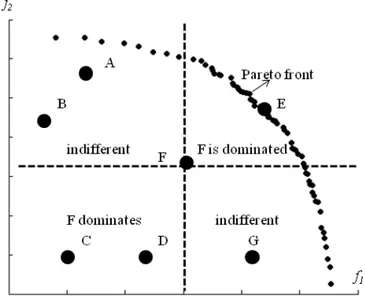
Examples of the concept of Pareto dominance and Pareto front are depicted in a graphical form in Figure 1.

(28)

It can be noticed that solutionF dominates solutionCandD, solutionF is dominated

byE, F is not comparable with A, BandG, solution E is non-dominated and Pareto optimal.

Note that a solution is a decision vector that has its Pareto dominance criteria based on the objective space (objective vector corresponding values).

Generating the Pareto set can be computationally expensive and it is often infeasible, because most of the time the complexity of underlying application prevents exact methods from being applicable. For this reason, a number of stochastic search strategies such as EAs, tabu search, simulated annealing, and ant colony optimization have been developed: they usually do not guarantee the identification of optimal trade-offs instead they try to find a good approximation, i.e., a set of solutions whose objective vectors are not too far from the Pareto optimal front (ZITZLER et al., 2004). Due to their population-based nature, EAs are able to approximate the whole Pareto front of a MOP in a single run, and these EAs are called MOEAs (ZHOU et al., 2011).

MOEAs have been well established as effective approaches to deal with MOPs (JIANG et al., 2015). After multiple trade-off and non-dominated points are found, higher-level information can be used to choose one of the obtained trade-off points (DEB, 2001).

Based on various acceptance rules to accomplish fitness assignment and selection to guide the search toward the Pareto-optimal set, and to maintain a diverse population achieving a well distributed Pareto front, classical MOEAs can be generally divided in Pareto dominance-based approaches, Scalarizing function-based methods and other approaches (JIANG et al., 2015).

2.2 PARETO DOMINANCE-BASED APPROACHES

There are many papers presenting various approaches to find a Pareto front, most of them based on classical MOEAs. The balance between convergence and diversity is the most important aspect while solving a MOP. Unlike single-objective-optimization, fitness calculation in MOPs is usually related to the whole population. The multi-objective optimization is a typical multimodal search aiming to find multiple different solutions in a single run.

(29)

sorting the population according to the dominance relationships established among solutions, producing a total ofTotF sub-populations or fronts, F1,F2, ...,FTotF. Front F1 corresponds to the set of non-dominated solutions (the best front). Each set Fi, i=2, ...,TotF, contains the

non-dominated solutions when setsF1, ...,Fi−1are removed from the current population.

A wide review of basic approaches and the specification of original Pareto evolutionary algorithms includes the works of Coello (1996) and Zitzler and Thiele (1999), where the last one describes the original Strength Pareto Evolutionary Algorithm (SPEA). An extension of the SPEA algorithm resulted in SPEA2 (ZITZLER et al., 2001) and Pareto Envelope-Based Selection Algorithm (PESA) (CORNE et al., 2000). This algorithm was updated to Pareto Envelope-Based Selection Algorithm II (CORNE et al., 2001), where the authors described a grid-based fitness assignment strategy in environmental selection. Another improved version, called IPESA-II (LI et al., 2013) introduced three improvements in environmental selection, regarding the performance: convergence, uniformity, and extensity.

One of the most popular approaches based on Pareto dominance is NSGA-II (DEB et al., 2002). Recently, its reference-point based variant, referred as NSGA-III (DEB; JAIN, 2014) was suggested to deal with many-objective problems, where the maintenance of diversity among population members is aided by supplying and adaptively updating a number of well-spread reference points.

We can point out the fact that Pareto approaches simultaneously consider all the objectives - every point/solution of the Pareto front is part of the set of solutions - and maintain the diversity of solutions. However two main disadvantages are that these approaches are computationally expensive and they are not very intuitive when the number of objectives is large. All the previously mentioned algorithms evolve toward the Pareto set with a good distribution of solutions but none of them guarantees the convergence to Pareto front.

2.3 SCALARIZING FUNCTION-BASED METHODS AND OTHERS APPROACHES

(30)

SMS-EMOA is a hypervolume-based algorithm. Its high search ability for many-objective problems has been demonstrated in the literature (WAGNER et al., 2007). The basic idea of SMS-EMOA is to search for a solution set with the maximum hypervolume for its corresponding objective vectors. In SMS-EMOA, two parents are randomly selected from a current population of sizeN to generate a single solution by crossover and mutation. The next

population with N solutions is constructed by removing the worst solution from the merged

population with(N+1)solutions. In the same manner as in NSGA-II, a rank is assigned to each solution in the merged population as the primary criterion to select individuals. Each solution with the same rank is evaluated by its hypervolume contribution as the secondary criterion.

In HypE, as in NSGA-II, first the non-dominated sorting is applied and then a criterion is used to select individuals among those with the same rank. The main difference is that the hypervolume maximization is used as the secondary criterion in environmental selection. Solution selection for the hypervolume maximization is performed in an approximate manner using Monte Carlo simulation given a number of sampling points.

MOEA/D is an efficient scalarizing function-based algorithm. A multi-objective problem is decomposed into a number of single-objective problems. Each single-objective problem is defined by the same scalarizing function with a different weight vector. The number of the weight vectors is the same as the number of the single-objective problems, which is also the same as the population size. A single solution is stored for each single-objective problem (ZHANG; LI, 2007).

There are several approaches for converting the problem of approximation of the Pareto front into a number of scalar optimization problems. In the following, we introduce three of them.

2.3.1 WEIGHTED SUM APPROACH

This approach considers a combination of the different objectives function

f1(x), ...,fR(x). Letλλλ = (λ1, ...,λR)T be a weight vector, i.e.λr≥0, for allr=1, ...,RwhereR

is the number of objectives and∑R_r₌₁λr=1. Then, the optimal solution to the following scalar

optimization problem:

maximize zws(x|λλλ) =∑R_r₌₁λrfr(x),

(31)

zws(x|λλλ) is a Pareto optimal point to Equation 11, λλλ is a weight vector in the zws

objective function, while x is the vector of variables to be optimized. To generate a set of different Pareto optimal vectors, we can use different weight vectors λλλ in this scalar optimization problem (MIETTINEN, 1999). If the Pareto front is concave (convex in the case of minimization), this approach could work well. However, not every Pareto optimal vector can be obtained by this approach in the case of nonconcave Pareto fronts (ZHANG; LI, 2007). To overcome these shortcomings, some effort has been made to incorporate other techniques such asε-constraint into this approach, more details can be found in Miettinen (1999).

2.3.2 TCHEBYCHEFF APPROACH

Another well-known method is the Tchebycheff Approach, for which scalar optimization problem uses theztefunction in the form:

minimize zte(x|λλλ,z∗) =max{λr|fr(x)−z∗r|},

subject to x∈X (3)

wherez∗= (z∗₁, ...,z∗_R)T _{is the ideal point in the decision space, i.e.,} _z∗

r =max{fr(x)|x∈X}2

for eachr=1, ...,R. For each Pareto optimal pointx∗there exists a weight vectorλλλ such that x∗ is the optimal solution of Equation 3 and each optimal solution of Equation 3 is a Pareto optimal solution of Equation 1. Therefore, the method is able to obtain different Pareto optimal solutions by altering the weight vector. One weakness with this approach is that this aggregation function is not smooth for a continuous MOP (ZHANG; LI, 2007).

2.3.3 BOUNDARY INTERSECTION APPROACH

Several recent MOP decomposition methods such as Normal-Boundary Intersection Method (DAS; DENNIS, 1998) and Normalized Normal Constraint Method (MESSAC et al., 2003) can be classified as Boundary Intersection (BI) approaches. They were designed for a continuous MOP. Under some regularity conditions, the Pareto front of a continuous MOP is part of the most top right 3 _{boundary of its attainable objective set. Geometrically, these}

BI approaches aim to find intersection points of the most top boundary and a set of lines. If these lines are evenly distributed in a sense, one can expect that the resultant intersection points provide a good approximation to the whole Pareto front. These approaches are able to deal

1_{If Equation 1 is for minimization, "maximize" in 2 should be changed to "minimize".} 2_{In the case of minimization,}_z∗

r =min{fr(x)|x∈X}

(32)

with nonconcave Pareto fronts. Mathematically, we consider the following scalar optimization subproblem withzbi function4:

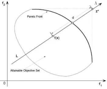
minimize zbi(x|λλλ,z∗) =d, subject to z∗−f(x) =dλλλ,

x∈X (4)

where λλλ and z∗, as in the previous subsection, are a weight vector and the ideal point, respectively. As illustrated in Figure 2, the constraint z∗−f(x) = dλλλ ensures that f(x) is always inL, the line with directionλλλ and passing throughz∗. The goal is to pushf(x)as high as possible so that it reaches the boundary of the attainable objective set (ZHANG; LI, 2007).

Figure 2: Ilustration of the boundary intersection approach (ZHANG; LI, 2007).

Appendix B contains some cutting edge detailed algorithms implemented in this work for further comparison.

2.4 SOLUTION QUALITY INDICATORS

Comparing different optimization techniques always involves the notion of performance. In the case of multi-objective optimization, the definition of solution quality is substantially more complex than for single-objective optimization problems, because the optimization goal itself consists of multiple objectives (ZITZLER et al., 2000):

• The distance of the resulting approximated Pareto-front to the Pareto optimal front should

(33)

be minimized (i.e., convergence);

• A good (in most cases uniform) distribution of the objective vectors found in the objective space is desirable. The assessment of this criterion might be based on a certain distance metric;

• The spread of the approximated Pareto-front should be maximized along the Pareto optimal front (i.e., diversity).

According to Martí-Orosa (2011), the stochastic nature of EAs prompts the use of statistical tools in order to reach a valid judgement of the solutions quality and how different algorithms compare with each other. The straightforward approach to experimental design is to run the algorithm for a given number of independent executions and then extract descriptive statistics of the performance indicators. These statistic measures can be used to support a given hypothesis.

A statistical hypothesis testing is used to determine significant differences between algorithms. This test generates the probability, p-value, of supporting a null hypothesis

according to a threshold probability: the significance level α. Regarding MOEA testing, it is desired to evaluate MOEAs by approximated Pareto sets.

There is a rather broad set of hypothesis test techniques. They can be grouped in parametric and non-parametric tests. According to García et al. (2008), in order to use the parametric tests it is necessary to check the following conditions:

• Independence: in statistics, two events are independent when the fact that one occurs does not modify the probability of the other one occurring;

• Normality: an observation is normal when its behaviour follows a normal or Gaussian distribution with a certain value of average µ and varianceσ2. A normality test applied over a sample can indicate the presence or absence of this condition in observed data. García et al. (2008) proposes three normality tests:

– Kolmogorov-Smirnov: it compares the accumulated distribution of observed data with the accumulated distribution expected from a Gaussian distribution, obtaining the p-value based on both discrepancies.

– Shapiro-Wilk: it analyzes the observed data to compute the level of symmetry and kurtosis (shape of the curve) in order to compute the difference with respect to a Gaussian distribution afterwards, obtaining the p-value from the sum of the squares

(34)

– D’Agostino-Pearson: it first computes the skewness and kurtosis to quantify how far from Gaussian the distribution is in terms of asymmetry and shape. It then calculates how far each of these values differs from the value expected with a Gaussian distribution, and computes a single p-value from the sum of these discrepancies.

• Heteroscedasticity: this property indicates the existence of a violation of the hypothesis of equality of variances. Levene’s test (LEVENE, 1960) can be used for checking whether or notksamples present this homogeneity of variances (homoscedasticity).

Non-parametric tests can be used for comparing algorithms whose results represent average values for each problem. Given that the non-parametric tests do not require explicit conditions for being conducted, it is recommendable that the sample of results is obtained following the same criteria, that is, computing the same aggregation (average, mode, etc.) over the same number of runs for each algorithm and problem.

Non-parametric tests consist of two meta-level approaches: rank tests and permutation tests. Rank tests pool the values from several samples and convert them into ranks by sorting them, and then they build tables describing the limited number of ways in which ranks can be distributed (between two or more algorithms) to determine the probability that the samples come from the same source. Permutation tests use the original values without converting them to ranks but explicitly estimate the likelihood that samples come from the same source by Monte Carlo simulation. Rank tests are the less powerful but are also less sensitive to outliers and computationally inexpensive. Permutation tests are more powerful because information is not discarded, and they are also better when there are many tied values in the samples, however they can be expensive to compute for large samples (CONOVER, 1999).

There are many statistical tests for MOEA quality indicators that can be used when comparing if two or more algorithms are different (better or worse) from another (KNOWLES et al., 2006; COELLO et al., 2007; ZITZLER et al., 2008). One of the most common non-parametric tests is the general form of the Mann-Whitney test called Kruskal-Wallis (KRUSKAL; WALLIS, 1952) H test, where K independent samples can be

compared. This statistical test can be performed for each comparable quality indicator using gathered experimental data (indicator values yielded by each algorithm’s run), and can determine if the samples are from the same population. This test is primarily used when no knowledge of the type of distribution is available. Expressing it more formally, for a set of algorithms A1, ...,AK, each one running nr times (from a total of Nr=nrK) on the same

problem, letIk,jbe the indicator value yielded by algorithmkin run j. In a particular problem (or

(35)

function that returns the position of measurementIk,jin the list. Following that, the rank sum is

calculated for each algorithm according to Equation 5:

˜Rankk= nr

∑

j=1

˜Rank(Ik,j);k=1, ...,K (5)

The definition of the Kruskal-WallisH test is reflected in Equation 6.

H = 12

Nr(Nr+1)

K

∑

k=1

˜Rank2_k

Nr_k −3(Nr+1) (6)

Given:

K sample of different sizes Nr1,Nr2, ...,NrK, where Nr = ∑Kk=1Nrk. When

Nr1,Nr2, ...,NrK =nrandNr=nrK, all algorithms runs the samenrtimes.

Upon calculation ofHusing Equation 6, its value is treated as though it was a value of

chi-square (χ2) sampling distribution with the degrees of freedom(d f) =K−1, meaning that as the test statisticHis approximatelyχ2-distributed, the null hypothesis is reject ifH>χ_K2₋_1;_α (ifH value is too great to fit inχ2distribution).

In case that the null hypothesis is rejected the Dunn-Sidak post-hoc test (CONOVER, 1999) can be applied in a pairwise manner in order to determine if the results of one algorithm are significantly better than those of the other. Dunn (1964) has proposed a test for multiple comparisons of rank sums based on the z statistics of the standard normal distribution and

proved accurate by Sidak (HOCHBERG; TAMHANE, 1987). In particular, the difference of indicator values yielded by algorithmsAk andAhis statistically significant if

|˜Rankk−˜Rankh|>z1−α/2∗ s

Nr(Nr+1) 12

1

Nrk

+ 1

Nrh

(7)

withz₁₋_α_/₂_∗defined as the value of the standard normal distribution for a given adjustedα/2∗ level.

(36)

2.4.1 HYPERVOLUME INDICATOR - HV

Hypervolume was introduced by Zitzler et al. (2003) and considers the size of the portion of the objective space that is dominated by the corresponding solutions region as an indicator of convergence (DEB, 2011).

Let Re f be a set of distributed points (objective vectors) in a reference set and AP

the approximated Pareto-front in the objective space obtained from the set of non-dominated solutionsNDin the variable space. HV∗(.)is the portion of the objective space whose solutions are dominated by the corresponding solutions from the set defined in the function argument. It can be defined as:

HV−(AP) =HV∗(Re f)−HV∗(AP) (8)

Note that we consider the hypervolume difference to the Re f. So, smaller values of

HV−(AP)correspond to higher quality solutions in non-dominated sets and they indicate both a better convergence as well a good coverage of the reference set (YAN et al., 2007; ARROYO et al., 2011).

2.4.2 INVERTED GENERATIONAL DISTANCE - IGD

The IGD is the average distance from each point on the reference set to the nearest point in the approximated set (in the objective space) (CZYZ ˆZAK; JASZKIEWICZ, 1998).

This metric measures both convergence and diversity (YEN; HE, 2014). LetRe f be a

set of distributed points (objective vectors) in the reference set. TheIGD(AP)for theNDset is:

IGD(AP) = ∑v∈Re fd(v,AP)

|Re f| (9)

where d(v,X), denotes the minimum Euclidean distance between pointv inRe f and

the points inAP. To have a low value of IGD, the set AP should be close to Re f and cannot

miss any part of the wholeRe f. The less the IGD, the better the algorithm’s performance.

2.4.3 CAPACITY METRICS

(37)

Non-dominated Vector Generation (ONVG) (VELDHUIZEN; LAMONT, 2000), given by Equation 10:

ONV G=|AP| (10)

In general, a large number of non-dominated solutions in AP is preferred (JIANG et

al., 2014). However, counting the number of non-dominated solutions inAP does not reflect

how farAPis fromRe f (VELDHUIZEN; LAMONT, 2000).

The Error Ratio (ER) (VELDHUIZEN; LAMONT, 1999), also used as a capacity metric, considers the solution intersections betweenAPandRe f, given by Equation 11:

ER=1−|AP∩Re f|

|Re f| (11)

whereAP∩Re f denotes the solutions existing in bothAPandRe f.

In this work, these metrics are obtained considering the non-dominated solutions gathering all executions from each algorithm.

2.5 SUMMARY

(38)

3 ESTIMATION OF DISTRIBUTION ALGORITHM - EDA

Claimed as a paradigm shift in the field of EA, EDAs are population based optimization algorithms, which employ explicit probability distributions (LARRAÑAGA; LOZANO, 2002). This chapter provides a brief introduction to EDAs, followed by a description of Bayesian Network, which is considered the most prominent Probabilistic Graphical Model (LARRAÑAGA et al., 2012).

The main idea of EDAs (MÜHLENBEIN; PAAB, 1996; LARRAÑAGA; LOZANO, 2002) is to extract and represent, using a PGM, the regularities shared by a subset of high-valued problem solutions. The PGM then samples new solutions guiding the search toward more promising areas.

EDAs have achieved good performance when applied to several problems (PHAM, 2011) including environmental monitoring network design (KOLLAT et al., 2008), protein side chain placement problem (SANTANA et al., 2008) and table ordering (BENGOETXEA et al., 2011). In the context of Travelling Thief Problem (TTP), other probabilistic models have been recently explored in a hyperheuristic framework using Genetic Programming (GP) (EL YAFRANI et al., 2017) and EDA (MARTINS et al., 2017b). Both approaches use well known low-level-heuristics in order to evolve combinations of these heuristics aiming to find a good model for the TTP instance at hand.

(39)

3.1 BASIC CONCEPTS

LetYm be a random variable. A possible instantiation ofYm is denoted byym, where

p(Ym=ym), or simply p(ym), denotes the probability that the variable Ym takes the value ym.

Y= (Y1, ...,YM) represents anM-dimensional vector of random variables, and y= (y1, ...,yM)

is a realization. The conditional probability ofymgivenyjis written as p(Ym=ym|Yj=yj)(or

simplyp(ym|yj). The joint probability distribution ofYis denoted by p(Y=y), or simply p(y).

In this section,Popdenotes a data set, or the set ofNinstantiations of the vector of the random

variablesY= (Y1, ...,YM).

The general framework of an EDA is illustrated in Figure 3.

Figure 3: The general framework of an EDA.

Usually, an EDA starts by generating a random population Pop of N solutions in

Initialize population Popblock. Each solution is an individualy= (y1, ...,yM)withMelements.

Solutions are then evaluated using one or more objective functions and, inSelect NPGM

individualsblock, a subset of them is selected according to a pre-defined criterion. PopPGM

represents the population of theNPGM individuals selected fromPop.

The selected solutions are used to learn a PGM in the block Estimate the probability

distribution using PGM, according p(y|PopPGM), that is, the conditional probability of a

(40)

at every generation. The most important step is to find out the interdependencies between variables that represent one point in the search space. The basic idea consists in inducing probabilistic models from the best individuals of the population.

Once the probabilistic model has been estimated, the model is sampled to generate a population Popsmp of new individuals (new solutions) in block Sample Popsmp for new

individuals using PGM. The cycle of evaluation, selection, modeling, and sampling is repeated

until a stop condition is fulfilled.

The steps that differentiate EDAs from other EAs are the construction of a probabilistic model and the process of sampling new candidate solutions based on the model. These blocks are highlighted in different color in Figure 3.

The next section introduces EDAs classification, based on the type of variables and the interdependencies that the PGM can account for (LARRAÑAGA; LOZANO, 2002).

3.2 CLASSIFICATION

Depending on the problem solution representation, EDAs can be categorized as discrete, permutation and real-valued based variables. Candidate solutions in EDAs have usually fixed length. However, variables can either be discrete or receive a real value that covers an infinite domain. Candidate solutions can also be represented by a permutation over a given set of elements, e.g. solutions for travelling salesman or quadratic assignment problem. This research concerns only EDAs for discrete variables. EDAs can be divided into three groups: Univariate, Bivariate and Multivariate according to the level of interactions among variables.

Univariate EDAs assume no interaction among variables. The joint probability mass function (pmf) of a solution y, which will be used afterward in the sampling process, is simply the product of univariate marginal probabilities of all M variables in that solution,

that is p(y) = ∏M_m₌₁p(ym). Algorithms in this category have simple model building and

sampling procedures and can solve problems where variables are independent. However, for problems with strong variable interactions, they tend to produce poor results. Different variants in this category include: Population-based Incremental Learning (PBIL) (BALUJA, 1994), Univariate Marginal Distribution Algorithm (UMDA) (MÜHLENBEIN; PAAB, 1996) and Compact Genetic Algorithm (cGA) (HARIK et al., 1999).

(41)

ordering of variables to address the conditional probabilities. These algorithms outperform univariate EDAs in problems with pair-wise variable interactions; however, they tend to fail when multiple interactions among variables exist in the problem (PHAM, 2011). Mutual Information Maximization for Input Clustering (MIMIC) (BONET et al., 1997), Combining Optimizer with Mutual Information Tree (COMIT) (BALUJA; DAVIES, 1997) and Bivariate Marginal Distribution Algorithm (BMDA) (PELIKAN; MUEHLENBEIN, 1999), all of them use bivariate models to estimate probability distribution.

Multivariate EDAs use probabilistic models able to capturing multivariate interactions between variables. Algorithms using multivariate models of probability distribution include: Extended Compact Genetic Algorithm (ECGA) (HARIK, 1999), Estimation of Bayesian Network Algorithm (EBNA) (ETXEBERRIA; LARRAÑAGA, 1999), Factorized Distribution Algorithm (FDA) (MÜHLENBEIN; MAHNIG, 1999), Bayesian Optimization Algorithm (BOA) (PELIKAN et al., 1999), Hierarchical Bayesian Optimization Algorithm (hBOA) (PELIKAN et al., 2003), Markovianity-based Optimization Algorithm (MOA) (SHAKYA; SANTANA, 2008), Affinity Propagation EDA (AffEDA) (SANTANA et al., 2010).

One of the most general probabilistic models for discrete variables used in EDAs and MOEDAs is the Bayesian Network (PEARL, 2000; KOLLER; FRIEDMAN, 2009), and we briefly describe it in the next section.

3.3 BAYESIAN NETWORK

Bayesian networks (BN) are directed acyclic graphs (DAG) whose nodes represent variables, and whose missing edges encode conditional independencies between variables. Random variables represented by nodes may be observable quantities, latent variables, unknown parameters or hypotheses. Each node is associated with a probability function that takes as input a particular set of values for the node’s parent variables and gives the probability of the variable represented by the node (COOPER; HERSKOVITS, 1992; KORB; NICHOLSON, 2010).

3.3.1 BASIC CONCEPTS

As in Section 3.1, let Y= (Y1, ...,YM) be a vector of random variables, and letym be

a value ofYm, the m-th component ofY. The representation of a Bayesian model is given by

two components (LARRAÑAGA et al., 2012): a structure and a set of local parameters. The set of local parametersΘcontains, for each variable, the conditional probability distribution of

(42)

The structure B for Y is a DAG that describes a set of conditional dependencies of all variables inY. PaB_m represents the set of parents (variables from which an arrow is coming out inB) of the variableYmin the PGM whose structure is given byB(BENGOETXEA, 2002).

This structure assumes thatYmis independent from its non-descendants givenPaBm,m=2, ...,M,

whereY1is the root node.

Therefore, a Bayesian network encodes a factorization for the mass probability as follows:

p(y) =p(y1,y2, ...,yM) = M

∏

m=1

p(ym|paBm) (12)

Equation 12 states that the joint pmf of the variables can be computed as the product of each variable’s conditional probability given the values of its parents.

In discrete domains, we can assume thatYmhassmpossible values,y1m, ...,ysmm, therefore

the particular conditional probability,p(yk_m|pamj,B), can be defined as:

p(yk_m|pa_mj,B) =θ_yk m|pa

j,B

m =θm jk (13)

wherepamj,B ∈ {pa1m,B, ...,pamtm,B}denotes a particular combination of values for PaBmandtm is

the total number of different possible instantiations of the parent variables ofYmgiven bytm=

∏_Y

v∈PaBmsv, where sv is the total of possible values (states) thatYv can assume. The parameter θm jk represents the conditional probability that variableYmtakes itsk−th value (ykm), knowing

that its parent variables have taken their j-th combination of values (pamj,B). This way, the

parameter set is given byΘ={θθθ1, ...,θθθm, ...θθθM}, whereθθθm= (θm11, ...,θm jk, ...,θm,tm,sm).

BN’s are often used for modeling multinomial data with discrete variables (PEARL, 1988) generating new solutions using the particular conditional probability described in Equation 13 (probabilistic logic sampling (HENRION, 1986)).

The next sections present a way to estimateΘparameters and theBstructure.

3.3.2 PARAMETER ESTIMATION

Generally, the parameters in the whole setΘare unknown, and their estimation process

is based on p(Θ|Pop,B), wherePopis the current data withN observations (instantiations) of

Y. Assuming a fixed structure B, let us consider the following assumption based on Bayes

(43)

p(Θ|Pop,B) = L(Θ;Pop,B)∗p(Θ|B)

p(Pop,B) (14)

In order to estimate theposteriori p(Θ|Pop,B)lets assume that the parametersθθθm j =

{θm j1,θm j2, ...,θm jsm}are independent (i.e. prioriandposterioriofΘcan be factorized through

θm j

θθm jm j) andNm jk is the number of observations inPopfor whichYmassumes the k-th value given

the j-th combination of values from its parents. According to this,Nm j={Nm j1, ...,Nm jsm}fits a multinomial distribution, with a pmf defined as follows.

p(Nm j|θθθm j,B) =

Nm j!

Nm j1!Nm j2!...Nm jsm! (θNm j1

m j1 )(θ Nm j2 m j2 )...(θ

N_{m jsm}

m jsm ) (15)

where∑sm

k=1Nm jk=Nm j and∑s_kmθm jk=1.

Considering the likelihood L(θθθm j;Pop,B) given by Equation 15, there are two

approaches to estimate each θm jk parameter: Maximum Likelihood Estimate (MLE) and

Bayesian Estimate.

With MLE, we expect to find a vector in Θ that maximizes the likelihood. We can

denote this vector as ˆθθθ. In MLE, each ˆθθθ ∈Θ is a point estimation, not a random variable.

Therefore, MLE does not consider any priori information, and the estimation is calculated

according to Equation 16, based on a frequentist analysis (by setting the derivative of Equation 15 to zero):

ˆ

θm jk=p(ykm|pamj,B,θθθm) =

p(Ym=ykm,pa j m)

p(pamj)

= f(y

k m,pa

j m)

f(pamj)

=Nm jk/Nm j (16)

where f(.)denotes the relative frequency and ˆθm jk is the MLE estimated parameter forθm jk.

Regarding to Bayesian estimation, it calculates theposterioridistribution p(Θ|Pop,B) considering aprioriinformationp(Θ|B). In practice, it is useful to require that the prior for each factor is a conjugate prior. For example, Dirichlet priors are conjugate priors for multinomial factors.

Considering we can assume that a priori θθθ fits a Dirichlet distribution with hyperparametersαααm j = (αm j1, ...,αm jsm) where αm jk ≥1, αm j =∑

sm

k=1αm jk and its expected

value is given by Equation 17:

(44)

Dirichlet prior can be written as the following density probability function:

p(θθθm j|B,αααm j) =

Γ(αm j)

Γ(αm j1)...Γ(αm jsm)

θαm j1−1

m j1 θ

αm j2−1

m j2 ...θ

α_{m jsm}−1

m jsm (18)

where Γ(.) is the Gamma function that satisfies Γ(x+1) = xΓ(x) and Γ(1) =1; according definitionΓ₍x) = (x−1)!, resulting inΓ₍1) = (1−1)!=1 and Γ₍x+1) =x!=x(x−1)(x− 2)...1=xΓ(x)(DEGROOT, 2005).

The term Γ(αm j)

Γ(αm j1)...Γ(αm jsm) can be considered a normalizer factor and Equation 18 can be rewritten as follows:

p(θθθm j|B,αααm j)∝θ

αm j1−1

m j1 θ

αm j2−1

m j2 ...θ

α_{m jsm}−1

m jsm (19)

Considering the priori as p(θθθm j|B,αααm j) and the likelihood as p(Nm j|B,θθθm j) , we

obtain the posteriori as p(θθθm j|αααm j,Nm j), given by Equation 20, which fits the Dirichlet

distribution with parametersαααm j= (αm j1+Nm j1, ...,αm jsm+Nm jsm).