Efficient methods for solving multi-rate partial differential equations in radio frequency applications

Efficient Methods for Solving Multi-Rate Partial Differential

Equations in Radio Frequency Applications

JORGE OLIVEIRA

Department of Electrical Engineering

Technology and Management School - Polytechnic Institute of Leiria Morro do Lena, Alto Vieiro, Apartado 4163, 2411-901 Leiria

PORTUGAL

oliveira@estg.ipleiria.pt

Abstract: - In telecommunication electronics, radio frequency applications are usually characterized by widely

separated time scales. This multi-rate behavior arises in many kinds of circuits and increases considerably the computation costs of numerical simulations. In this paper we are mainly interested in electronic circuits driven by envelope modulated signals and we will show that the application of numerical methods based on a multi-rate partial differential equation analysis will lead to an efficient strategy for simulating this type of problems.

Key-Words: - Electronic circuit simulation, envelope-modulated signals, multi-rate partial differential equations.

1 Introduction

Dynamical behavior of electronic circuits can in general be described by ordinary differential equations (ODEs) in time, involving electric voltages, currents and charges and magnetic fluxes. For a general nonlinear circuit, Kirchhoff's laws lead to the system

( )

( )

( ) ( )

( )

x t , dt t y dq t y p + = (1)

where

x t

( )

∈R

n and stand for the

excitation and state-variable vectors, respectively. represents memoryless linear or nonlinear

elements, while models dynamical linear or

nonlinear elements (capacitors or inductors).

( )

n

y t

∈ R

( )

(

y

t

p

)

)

( )

(

y

t

q

When the excitation is a multi-rate stimulus the simulation process of such circuits is often a very challenging issue, especially if they are highly nonlinear. In the particular case in which we are interested (envelope modulated excited circuits) it happens that while envelopes are slowly varying signals, carriers are usually very high frequency sinusoids. Thus, obtaining the numerical solution of (1) is difficult because once we have signals with widely separated rates of variation we are forced to make discretizations on long time grids with extremely small time steps.

( )

t

x

2 Multidimensional Problem

In this section we will begin by presenting a recent generic formulation for solving electronic circuits with widely separated time scales. As we will see, the key idea behind this strategy is to use multiple time variables, which enable multi-rate signals to be

represented more efficiently. In our case, we will need two time variables and we will adopt the following procedure: for the slowly-varying parts (envelope) of the expressions of

x

( )

t

and

y

( )

t

,

t

is replaced by

t

₁; for the fast-varying parts (carrier)

t

is

replaced by ₂. This will result in bivariate

representations for the excitation and the solution, and we will denote these two argument functions by

t

(

1

,

2

)

ˆ

t

t

x

and

ˆy

(

t

₁

,

t

₂

)

.

2.1 Bivariate Representation

Simulating circuits using numerical schemes require time steps spaced closely enough to represent signals accurately. For concreteness let us consider the

slowly-varying envelope signal shown in Fig.1

and let us suppose that it was plotted with 50 samples, that is to say, 50 points were necessary to represent

( )

e t

( )

e t

accurately. 0 0.1 0.2 0.3 0.4 0.5 0.6 0.7 0.8 0.9 1 0.5 1 1.5 2 2.5 3 3.5 4 t [s] e

Fig.1. Envelope signal e(t)

Let us also consider the envelope modulated signal

x t

( )

shown in Fig.2, defined by

( ) ( ) (

sin 2

_c

)

x t

=

e t

π

f t

,

with a carrier frequency

f

_c

=

1

T

₂ and let’s suppose that 20 points were used per sinusoid. In this case the total number of samples will be

N

=

20

× f

_c. So, if

we have for example kHz, then we will obtain samples. Obviously, this number can be much larger if we increase c

1

c

f

=

3 20 10 N = ×

f

(e.g.

f

c

=

1

MHz

would lead to N =20 10× 6 samples).

0 0.1 0.2 0.3 0.4 0.5 0.6 0.7 0.8 0.9 1 −4 −3 −2 −1 0 1 2 3 4 t [s] x

Fig.2. Envelope modulated signal x(t)

Consider now the bivariate representation for

( )

x t

denoted by

x t t

ˆ

(

₁

,

₂

)

and defined by

(

1 2

) ( ) (

1 2

ˆ

,

sin 2

_c

)

x t t

=

e t

π

f t

.

This function of two variables is periodic with respect to t₂, but not to , i.e. t₁

(

1 2

) (

1 2 2

ˆ

,

ˆ

,

)

x t t

=

x t t

+

T

.

The plot of

x t t

ˆ

(

₁

,

₂

)

on the rectangle

[ ] [

0,1

×

0,T

₂

]

for a carrier period ms ( kHz) is shown

in Fig.3 and because of its periodicity this plot repeats over the rest of the axis. We must note that

2 1 T = f_c =1 2 t

(

1 2

)

ˆ

,

x t t

doesn’t have many undulations, unlike

( )

x t

in Fig.2. Consequently, it can be represented by relatively few samples. In fact, if we consider the same 50 sample points for

e t

( )

( dimension) and the same 20 sample points for each carrier cycle ( dimension) then we will have now only

samples, independently of the frequency 1 t 2 t

50 20 1000

N

=

×

=

c

f . This is very significant, because

considerable computation and memory savings will result from this

N

reduction.

0 0.2 0.4 0.6 0.8 1 0 0.2 0.4 0.6 0.8 1 −4 −3 −2 −1 0 1 2 3 4 t 1 [s] t₂ [ms] x^

Fig.3. Bivariate representation x t tˆ

(

₁, ₂

)

Note that the original signal

x t

( )

can be easily recovered from its bivariate representation

x t t

ˆ

(

₁

,

₂

)

, simply by setting t1= =t2 t, that is to say,

( ) (

ˆ ,

)

x t

=

x t t

.

Consequently, due to the periodicity of the function

(

1 2

)

ˆ

,

x t t

in t₂ dimension, on the rectangular domain

[ ] [

0,1

×

0,T

2

]

we obtain

( ) (

ˆ , mod

2

)

x t

=

x t t

T

,

for any time value

t

∈

[ ]

0,1

. Observe that as t

increases from 0 to 1, the set of points given by

(

t t

, mod

T

2

)

traces the sawtooth path shown in

Fig.4. By noting how

x t t

ˆ

(

1

,

2

)

changes along this

path, the behavior of

x t

( )

can be visualized.

t2 [ms] 0 1 0 T2=1 . . . t1 [s]

Fig.4. Path on the rectangle

[ ] [

0,1 × 0, T₂

]

2.2 Multi-Rate Partial Differential System

The discussion presented above illustrates that in spite of the sampled bivariate signal involve far fewer points than its univariate form, it contains all the information needed to recover the original signal completely. This way the ordinary differential (ODE) system (1) will be converted to the multi-rate partial differential (MPDE) system

(

(

)

)

(

(

)

)

(

(

)

)

=

∂

∂

+

∂

∂

+

2 2 1 1 2 1 2 1

,

ˆ

,

ˆ

,

ˆ

t

t

t

y

q

t

t

t

y

q

t

t

y

p

=

x

ˆ

(

t

₁

,

t

₂

)

.

(2) Then, if we want the original univariate solution

y

( )

t

for a generic interval 0≤t≤t_s, we must solve (2) on the rectangular region

[ ] [

0,ts × 0,T2

]

of space,

with the following initial and boundary conditions:

2 1

,t

t

( ) (

0

,

,

ˆ

t

₂

g

t

₂

y

=

)

(3)

( ) (

,

0

ˆ

,

.

ˆ

t

₁

y

t

₁

T

₂

y

=

)

(4)

( )

⋅

g

is any given initial-condition function and (4) appears due to the periodicity of the problem in dimension. The univariate solution may then be

recovered from its bivariate form , simply by

setting 2

t

( )

t

y

(

1

,

2

ˆ

t

t

y

)

( ) (

t

y

ˆ

t

,

t

mod

T

2

)

y

=

.

The mathematical relation between the ODE system (1) and the MPDE system (2) is established by the following theorems:

Theorem 1 If

y

ˆ

(

t

₁

,

t

₂

)

and

x t t

ˆ

(

₁

,

₂

)

satisfy the MPDE system (2), then

y t

( )

=

y t

ˆ

(

+

c t

₁

,

+

c

₂

)

and

( ) (

ˆ

1

,

2

)

x t

=

x t

+

c t

+

c

satisfy the ODE system (1), for any fixed

c c

₁

,

₂

∈ R

.

Proof: Since

q y t

(

( )

)

=

q y t

(

ˆ

(

+

c t

₁

,

+

c

₂

)

)

, then we have

( )

(

)

(

(

)

)

(1 2) ( 1 2) 1 2 ₁ 1 , ,

ˆ

,

t t t c t c

dq y t

q y t t

_dt

dt

t

dt

= + +

∂

=

⋅

∂

+

(

)

(

)

(1 2) ( 1 2 1 2 2 2 , ,

ˆ

,

t t t c t c

q y t t

_dt

t

d

= + +

∂

+

∂

)

t

⋅

. Now, once dt1 dt2 1 dt = dt = , according to (2) we obtain

( )

(

)

₍

₎

(1 2) ( 1 2) 1 2 _{, ,}

ˆ

,

t t t c t c

dq y t

x t t

dt

=

= + +

(

)

(

)

_{( ) ( )} 1 2 1 2 1 2 _{, ,} ˆ , t t t c t c p y t t = + + − , that is to say,

( )

(

)

₍

₎

₍

₍

( )

(

( )

)

1 2 1 2 ˆ , ˆ dq y t

)

)

, x t c t c p y t c t c dt x t p y t = + + − + + = − and consequently

( )

(

)

dq y t

(

( )

)

( )

p y t

x t

dt

+

=

.

Theorem 2 If the ODE system (1) has a unique

solution

y

( )

t

for an excitation

x t

( )

given any initial condition, then the solution of the MPDE

system (2) is also unique (if it exists), given the initial and periodic boundary conditions (3) and (4).

(

1

,

2

ˆ

t

t

y

)

)

Proof: Theorem 1 tells us that the one-dimensional

solutions are given by ,

meaning that they are obtained along diagonal lines

in the space, where are

the MPDE solutions with an initial condition

( )

t

y

y t

( )

=

y t

ˆ

(

+

c t

₁

,

+

c

₂

)

(

t

+

c t

1

,

+

c

2

)

t t

1

,

2

y

ˆ

(

t

1

,

t

2

( )

0

y

given by . Thus, on the

diagonal lines passing through each point

(

)

in the initial condition region

( )

0

ˆ

(

1

,

2

)

( )

2

y

=

y c c

=

g c

1

,

2

c c

[

]

1

0,

c

×

T

₂ , the MPDE

has a unique solution, since the ODE has a unique solution. Now, in view of the fact that

y t t

ˆ

(

₁

,

₂

)

is periodic with respect to , its value at any point is equal to that at some point along one of the diagonal lines above (this leads to a sawtooth path on the rectangular region

2

t

(

t t

1

,

2

)

]

[ ] [

0

,

t

s

×

0

,

T

2 ). Consequently

the solution

y t t

ˆ

(

₁

,

₂

)

is unique.

3 Numerical Solution of the MPDE

We will now present some efficient methods for solving (2)-(4), based on the bivariate strategy introduced in the previous section. The first three ones operate purely in the time domain. The last one is used to solve the MPDE for ₁ dimension in the time domain and for dimension in the frequency domain.

t

2

t

3.1 Finite Differences Method

Let us consider the set of grid points

( )

j i

t

t

₁

,

₂ defined on the rectangle

[ ] [

0

,

t

s

×

0

,

T

2

]

by 0 1 1 1 1 1

0

,

i KS s

t

t

t

t

t

=

< <

< <

<

=

(5) 0 1 2 2 2 2 2 2

0

,

j K

t

t

t

t

T

=

<

<

<

<

<

=

(6) with 1 1i 1i 1i h = −t t ₋ and 1 2j 2j 2

h

t

t

− j

=

−

the grid spacings in the ₁ and ₂ directions,

respectively. By discretizing the partial differentia-tion operators of the MPDE collocated on the grid, we obtain a system of nonlinear algebraic equations that can be numerically solved using for example Newton-Raphson method. For instance, consider the finite difference approximation given by the backward Euler rule

t

t

( )

( )

(

)

( ) (

)

, ˆ ˆ ˆ 1 , 1 , , , 1 2 1 2 1 _{i j} hi y q y q t y q i j i j t t t t − = − ≈ ∂ ∂

( )

( )

(

)

( ) (

)

, ˆ ˆ ˆ 2 1 , , , , 2 2 1 2 1 _{i j} h j y q y q t y q i j i j t t t t − = − ≈ ∂ ∂ with

( )

j i

t

t

y

y

ˆ

_i,j

=

ˆ

₁

,

₂ . This leads for each level i, from

i

=

1

to

i

=

K

_S, to the scheme

,

0

ˆ

ˆ

ˆ

ˆ

ˆ

ˆ

_, 2 1 , , 1 , 1 , ,

−

=

−

+

−

+

− − j i j i j i j i j i j i

x

h

q

q

h

q

q

p

j i (7)

j

=

1

,

…

,

K

₂

,

where pˆ_i,j = p

( )

yˆ_i,j , qˆ_i,j =q

( )

yˆ_i,j and

( )

t

_i

t

_j

x

x

ˆ

_i,j

=

ˆ

₁

,

₂ . This way, knowing the initial

solu-tion on

i

=

0

(

t

₁

=

0

)

given by

( )

j

j 2

,

0 , we

can find the solution on each next level i by

iteratively solving (7).

t

g

yˆ

=

K We can rewrite (7) as , 0, 1, , 2 i j F = j= … , or, equivalently,

( )

0

i i

F Y

=

, with

2 ,1 ,2 , T i i i i K F = ⎣⎡F F F ⎤_⎦ and 2 ,1 ,2 , T i i i i K Y = ⎣⎡Y Y Y _⎦⎤

)

v .

If we choose for example the Newton-Raphson iterative solver, then on each iteration we have to solve the linear system

v

( )

[ ]v [v 1] [ ]v

(

[ ] i i i i i J Y ⋅⎡_⎣Y + −Y ⎤_⎦= −F Y where i i dF J dY =

is the Jacobian matrix of

F

i

( )

⋅

.

In the scalar case the Jacobian is a sparse matrix and according to (7) it’s not difficult to verify that it is given by 2

K

×

K

₂ 2 2 1 1 2 2 K K

D

L

L

D

J

L

D

⎡

⎤

⎢

⎥

⎢

⎥

=

⎢

⎥

⎢

⎥

⎢

⎥

⎣

⎦

where ' ' , , ' , 1 2 ˆ ˆ ˆ i j i j i j j i j q q D p h h = + + and ' , 1 2 ˆ j i j j q L h − = − , with pˆ_{i j}'_, = p'

( )

yˆ_{i j,} and qˆ_{i j}'_, =q'

( )

yˆ_{i j,} .

3.2 Method of Lines

Consider the semi-discretization of

[ ] [

0

,

t

_s

×

0

,

T

₂

]

defined by (6). Thus, by discretizing the MPDE (2) only in , we obtain an ordinary differential system in dimension, that can be time-step integrated with an initial value solver (e.g. Runge-Kutta [1]). If we use, once again, finite difference approximations based on the backward Euler rule then we have

2

t

1

t

(

( )

)

+

(

( )

)

+

(

( )

)

−

(

−

( )

)

=

j

h

t

y

q

t

y

q

dt

t

y

dq

t

y

p

_j j j j 2 1 1 1 1 1 1

ˆ

ˆ

ˆ

ˆ

( )

, 1, , , ˆ t₁ j K₂ x_j = … = (8) where

( )

( )

j

t

t

y

t

y

ˆ

_{j 1}

=

ˆ

₁

,

₂ and

( )

( )

j

t

t

x

t

x

ˆ

_{j 1}

=

ˆ

₁

,

₂ .

Now, according to the chain rule

( )

(

)

( )

( )

, ˆ ˆ 1 ' ˆ 1 1 1 t y dy dq dt t y dq j t y y j j = =

(8) can be described in the classical form

( )

( )

0, 1 1

ˆ

0

ˆ

,

0

,

ˆ

,

'

ˆ

y

y

t

t

y

t

f

y

_s

=

≤

≤

=

which in this case results in

( )

( )

(

( )

)

(

( )

)

(

( )

)

⎥ ⎥ ⎦ ⎤ ⎢ ⎢ ⎣ ⎡ − − − = 1 2 2 1 1 1 1 1 1 1 1 ' 1 ˆ ˆ ˆ ˆ ˆ h t y q t y q t y p t x t y K ( ) 1 ˆ1 1 − = ⎥ ⎥ ⎦ ⎤ ⎢ ⎢ ⎣ ⎡ t y y dy dq

( )

( )

(

( )

)

(

( )

)

(

( )

)

2 2 1 1 1 ' 2 1 2 1 2 1 2 ˆ ˆ ˆ ˆ ˆ q y t q y t y t x t p y t h ⎡ − ⎤ =⎢ − − ⎥ ⎢ ⎥ ⎣ ⎦ ( ) 2 1 1 ˆ y y t dq dy − = ⎡ ⎤ ⎢ ⎥ ⎢ ⎥ ⎣ ⎦

( )

( )

(

( )

)

(

( )

)

(

( )

)

⎥ ⎥ ⎦ ⎤ ⎢ ⎢ ⎣ ⎡ ₋ − − = − 2 2 2 2 2 2 2 1 1 1 1 1 1 ' _{ˆ ˆ} ˆ ˆ ˆ K h t y q t y q t y p t x t y_{K K K} K K ( ) 1 ˆ 2 1 − = ⎥ ⎥ ⎦ ⎤ ⎢ ⎢ ⎣ ⎡ t y y K dy dq with

( )

( )

1 2 0 2 2

ˆ

,

,

K T

y

= ⎣

⎡

g t

…

g t

⎤

_⎦

.

3.3 Shooting

Consider now the semi-discretization of the rectangle

[ ] [

0

,

t

s

×

0

,

T

2

]

defined by (5). By discretizing the

MPDE (2) only in ₁ dimension, we obtain for each level

i an ordinary differential system in 2, with

periodic boundary conditions. If we use again the backward Euler rule then we have for each i, from

t

t1

t

1

=

i

to

i

=

K

S, the boundary value problem

( )

(

)

+

(

( )

)

−

(

−

( )

)

+

(

( )

)

= 2 2 1 2 1 2 2 ˆ ˆ ˆ ˆ dt y dq h t y q t y q t y p i i i i i t

( )

,

ˆ

t

₂

x

i

=

(9)

( )

0

ˆ

(

,

ˆ

y

T

₂

y

i

=

i

)

(10) where yˆ

( )

t₂ yˆ

( )

t₁ ,t₂ i i = and xˆi

( )

t2 xˆ

( )

t1_i,t2 . This

means that once

=

( )

2

1

ˆ

t

y

_i− is known, the solution on next level,

y

ˆ t

_i

( )

₂ , is achieved by solving (9)-(10). However, we must note that if we use an initial value solver (Runge-Kutta or another time-step integrator) with step size control (automatically adjusting its step lengths in order to achieve a prescribed tolerance for the error), then we will have an irregular grid with different grid point values ₂

j (unequal discretizing

of the ₂ time axis) on successive levels ₁

i . This

means that when solving (9)-(10) we have to

interpo-late the numerical solution for obtaining the

t

t

t

( )

1 2

ˆ

_i

y

₋

t

numerical solution . Nevertheless, obviously

for obtaining the whole solution in the entire

domain we have to solve a totality of

S boundary value problems. Here we propose to

solve (9)-(10) using classical shooting [2], [5].

( )

2

ˆ

_i

y t

ˆy

[ ] [

0

,

t

s

×

0

,

T

2

]

)

K

Shooting is an iterative solver that uses an initial value technique to solve a boundary value problem. In our case we have periodic boundary conditions and the problem can be formulated in the following way: what initial condition, or left boundary , should be selected for time-step integration, that would lead to a final condition, or right boundary, satisfying ? Shooting is, in fact, a procedure that consists in guessing the initial estimate, by comparing and wisely updating the initial condition after successive time-step integrations. One possible way to do so consists in starting from a predetermined

and successively making

( )

0

ˆ

_i

y

( )

ˆ

(

0

ˆ

_i

T

₂

y

_i

y

=

( )

[0]

ˆ

_i

0

y

( )

( )

( )

( )

[1] [0] [2] [1] 2

ˆ

_i

0

ˆ

_i

,

ˆ

_i

0

ˆ

_i

,

y

=

y

T

y

=

y

T

₂

…

T

that is to say,

( )

( )

[ 1] [ ] 2

ˆ

v

0

ˆ

v i i

y

+

=

y

, until

( )

( )

[ ] [ ] 2 ˆif ˆif 0 y T −y <Tol n ,

with a permitted tolerance for the error. If we

define , such that

Tol

:

n

φ

R

→

R

( )

2

(

( )

)

ˆ

_i

ˆ 0

_i

y T

=

φ

y

,

then this natural initial condition update algorithm can be understood as the iterative solving of

( )

(

y

ˆ

_i

0

)

y

ˆ

_i

( )

φ

=

0

(11) using the fixed point iteration method.

Another way to guess the initial condition

y

ˆ

_i

( )

0

consists in making use of the Newton-Raphson iterative solver to get the solution of (11). In such case, rewriting (11) as

( )

(

ˆ

_i

0

)

(

ˆ

_i

( )

0

)

ˆ

_i

( )

0

F y

=

φ

y

−

y

=

0

Newton iterations take the form

( )

( )

(

( )

)

(

( )

)

[ 1] [ ] 1 [ ] [ ]

ˆv 0 ˆv 0 ˆv 0 ˆv

i i i i

y + =y −J− y ⋅F y 0 ,

where the Jacobian matrix is given by

( )

(

)

_{( )}

(

( )

)

( )

(

( )

)

[ ] [ ] [ ]

ˆ

0

ˆ

0

ˆ 0

ˆ

0

ˆ 0

v v i i i v i i

dF

J y

y

dy

d

y

I

dy

φ

=

=

−

with I the

n

identity matrix. In practice, it is more efficient not to invert but instead use for example LU decomposition to solve, at each step of the iteration, the linear algebraic system

n

×

J

( )

(

[ ]

)

[ 1]

( )

[ ]v

( )

(

[ ]

( )

)

ˆiv 0 ˆiv 0 ˆi 0 ˆiv 0 J y ⋅⎡_⎣y + −y ⎤_⎦= −F y .

Newton iteration is considerably more expensive on computing time than is fixed point iteration. Each step of the later costs just one function evaluation, whereas each step of the former calls for the updating of the Jacobian and a new LU decomposition and back substitution. However, if the function

φ

is linear or quasi-linear, the Newton-Raphson iterative solver becomes more efficient than the fixed point iteration method.

3.4 Mixed Frequency-Time Method

Let us return again to (9)-(10). We will now propose to solve each one of these boundary value problems using harmonic balance (HB) [2], [5]. HB is a classi-cal solver commonly used in RF and microwave circuit simulation, which uses a linear combination of sinusoids to build the solution, by expanding all waveforms in Fourier series.

For simplicity let us suppose, instead of (9)-(10), a general univariate boundary value problem with periodic boundary conditions, defined by

( )

(

)

dq y t

(

( )

)

( )

,

p y t

x t

dt

+

=

(12)

( )

0

( )

0

y

=

y T

.

(13) If the excitation

x t

( )

and the solution

y t

( )

are both periodic of fundamental frequency

ω

₀

=

2

π

T

₀ , they can be expressed by their Fourier series

( )

jk 0t_,

( )

jk 0t_. k k k k x t X e ω y t Y e ω +∞ +∞ =−∞ =−∞ =

∑

=

∑

(14)

Truncating the harmonics at

K

ω

₀ and substituting (14) in (12) we obtain 0 0 0

_.

K K jk t jk t k k k K k K K jk t k k K

d

p

Y e

q

Y e

dt

X e

ω ω ω + + =− =− + =−

⎡

⎤

⎛

⎞

⎛

⎞

+

_⎢

_⎥

=

⎜

⎟

⎜

⎟

⎝

⎠

⎣

⎝

⎠

⎦

=

∑

∑

∑

As it can be seen in detail for example in [5], the HB method consists in transforming this equation entirely to the frequency domain, in order to obtain

( )

=

( )

+

j

( )

−

0

F Y

P Y

ΩQ Y

X

=

, (15)

where and Y stand for the vectors with the

Fourier coefficients of the excitation and the solution

X

[

0

]

T K K X₋ X X = X

[

0

]

T K K Y₋ Y Y = Y and 0 0

0

0

0

jK

j

j

jK

ω

ω

−

⎡

⎤

⎢

⎥

= ⎢

⎥

⎢

⎥

⎣

⎦

Ω

.

The solution of the harmonic balance equation (15) is usually achieved by two similar iterative strategies, known as source stepping and harmonic-Newton algorithms. The first one tries to find the solution by successively solving partial linear problems obtained by increasing the magnitude of a reduced version of the excitation. The second one attempts to solve (15) by Newton-Raphson iteration for the full excitation, leading to

( )

1

(

[v+1]

=

[ ]v

−

⎡

[ ]v

⎤

−

⋅

[ ]

⎣

⎦

Y

Y

J Y

F Y

v

)

, until

( )

[ ]f

Tol

<

F Y

, where

( )

[ ] [ ] [ ] [ ] v v v v

d

d

j

=

=

=

+

Y Y

F

J Y

Y

G

ΩC

with

G

and

C

the Toeplitz [5] matrices of

dp dy

and

dq dy

, respectively.

Now let us return to the problem (9)-(10). In this

case, for each time-step we will have an HB

equation i t₁

( ) ( ) ( )

ˆ

ˆ

ˆ

( )

ˆ

ˆ

,

1 1 i i i i i

j

h

i

X

Y

ΩQ

Y

Q

Y

Q

Y

P

+

−

−

+

=

where and are the vectors with the Fourier

coefficients for the excitation and the solution on level . So, we have a mixed mode technique that handles the envelope ( dimension) in the time

domain and the carrier ( dimension) in the

frequency domain. i

Xˆ

Yˆ

_i i 1

t

2

t

4 Experimental Results

4.1 Sample Application

In order to test the efficiency of the methods presented in the previous section, we propose the nonlinear single node circuit of Fig.5.

Beyond the power source _S, this circuit is composed by a linear conductance, a nonlinear capacitance and a nonlinear current source. The characteristics of the nonlinear elements are modeled in the following way:

i

• For the current we considered a nonlinear voltage-dependent current source

( )

(

v

t

)

I

(

v

(

t

i

_{NL O}

=

₀

tanh

α

_O

))

. (16) • For the capacitance we considered that

( )

(

v

t

)

i

(

v

(

t

q

_{NL O}

=

τ

_{F NL O}

))

, (17)

which means that the storage charge is proportional to the conductive current. Thus,

( )

(

)

(

_{( )}

( )

)

( )

(

)

2 0

sech

.

NL O O O F O

dq

v

t

C v

t

dv

t

I

v

t

τ α

α

=

=

These nonlinear models are usually encountered in doped semiconductors (e.g. saturating velocity field resistors and junction diffusion capacitances). The forms of

i

_NL

(

v

_O

( )

t

)

and

C v

(

_O

( )

t

)

are plotted in Fig.6 and Fig.7, respectively.

G

vO(t)

i_S(t) qNL(vO(t)) iNL(vO(t))

Fig.5. Nonlinear circuit example

v_O(t) i_NL(v_O(t)) 1/α −1/α I₀ −I₀

Fig.6. Nonlinear current

v_O(t)

C(v_O(t))

1/α −1/α

τ_FαI₀

Fig.7. Nonlinear capacitance

4.2 Mathematical Model

The mathematical model of an electronic circuit is based on Kirchhoff’s current and voltage laws:

• Kirchhoff’s current law: “The net current into any node is zero”.

• Kirchhoff’s voltage law: “The net sum of the voltage drops around any closed loop is zero”.

In this case we have a simple single node circuit and we only need to apply the Kirchhoff’s current law to the node O. Doing so, we can say that the nodal

analysis of the circuit leads to

v

G C NL

i

+ +

i

i

=

i

_S. (18) The conductance

G

is assumed as linear and is thus characterized by a proportional relation between its terminal voltage and current, that is to say,

( )

( )

G O

i

t

=

Gv

t

, (19) known as Ohm’s law. For the nonlinear capacitance we have

( )

NL

(

O

( )

)

C

dq

v

t

i

t

dt

=

(20)

for the fundamental relation between its current and charge. Substituting (19) and (20) in (18) we obtain the following ordinary differential equation:

( )

(

( )

)

i

(

v

( )

t

)

i

(

t

.

dt

t

v

dq

t

Gv

NL O _{NL O S} O

+

+

=

)

ce the nonline

Finally, sin ar charge

q

_NL

(

v

_O

( )

t

)

)

and

current are modeled by (17) and (16), we

can write

( )

(

NL O

i

v

t

( )

0

sech

2

(

( )

)

( )

O O F O

dv

t

Gv

t

I

v

t

dt

ατ

α

+

+

( )

(

)

( )

0

tanh

O S

I

α

v

t

i

t

+

=

. (21)

4.3 Numerical Simulation Results

The circuit of Fig.5 was simulated in MATLAB® from

to ms, for

0

=

t

t

=

1000

G

=

1

mΩ-1 ,

I

0

=

0

.

4

mA,

1

=

α

V-1,

τ

_F

=

2

⋅

10

−3s and an excitation

( ) ( ) (

t

e

t

f

t

)

i

_S

=

sin

2

π

_c mA,

with a carrier frequency

f

c

=

1

kHz and an envelope

( )

t

(

f

t

)

e

=

5

sin

2

π

, f =0.5Hz.

The values of

G

,

I

₀,

α

and

τ

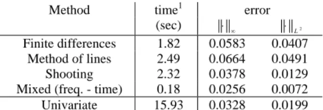
_F were chosen in way to obtain a considerably nonlinear problem and the overall results of this simulation are presented in Table 1 where, for comparison, we also included a non multi-rate method (classical univariate time-step integration). As we can see, the multi-rate methods presented in Section 3 exhibit significant advantages in speed over the non multi-rate method. In fact, while in the MPDE based methods we have total computation times ranging from 0.18 to 2.49 seconds, in the univariate time-step integration we have 15.93 seconds.

In order to test the accuracy of the methods a reference solution was achieved by numerically solving the ODE (21) via classical univariate time-step integration, using an embedded Runge-Kutta [1] method of higher order, with an extremely small time step.

Method time1 error

(sec) ⋅ ∞ ⋅ _L2

Finite differences 1.82 0.0583 0.0407

Method of lines 2.49 0.0664 0.0491

Shooting 2.32 0.0378 0.0129

Mixed (freq. - time) 0.18 0.0256 0.0072

Univariate 15.93 0.0328 0.0199

Table 1. Numerical simulation results

The bivariate solution is shown in Fig.8 and the univariate solution is of the type of the one plotted in Fig.9. 0 200 400 600 800 1000 0 0.2 0.4 0.6 0.8 1 −2 −1.5 −1 −0.5 0 0.5 1 1.5 2 t₁ [ms] t₂ [ms] v_O ^

Fig.8. Bivariate solution, vˆO

(

t t1, 2

)

0 100 200 300 400 500 600 700 800 900 1000 −2 −1.5 −1 −0.5 0 0.5 1 1.5 2 t[ms] vO

Fig.9. Univariate solution v_O

( )

t

In order to have a more realistic and accurate idea of the solution, a time scaled version of

v

_O

( )

t

in the interval [498,500]ms is plotted in Fig.10. The reason why we chose this particular interval is because the nonlinearity effects are stronger here (maximum excitation).

1

Computation time (AMD Athlon 1.8 GHz, 256MB RAM).

498 498.2 498.4 498.6 498.8 499 499.2 499.4 499.6 499.8 500 −2 −1.5 −1 −0.5 0 0.5 1 1.5 2 t [ms] vO

Fig.10. Univariate solution v_O

( )

t , in [498,500]ms

We have tested other values of

G

,

I

0,

α

and

τ

F,

ding to weakly nonlinear and quasi-linear problems, and the results were similar to the ones presented in Table 1: multi-rate methods were always much faster than the univariate one and an excellent speedup was exhibited by the mixed (frequency-time) method. However, the extreme efficiency of this mixed method cannot be generalized. In fact, if for a fixed excitation we successively increase the value of lea

α

or decrease the values of

G

and

I

₀, the circuit nonlinearities become stronger and the method looses efficiency. We have simulated the problem with

mΩ

0.74

G

=

-1

,

I

₀

=

0.155

mA,

α

=

2

V-1 and

s, and we obtained a total of 4.98 seconds for the computation time of the mixed method, while for example in the finite differences method this time was 1.99 seconds. Furthermore, if we try to decrease the values of

G

or ₀

3 5 10 F

τ

_{= ⋅} −

I

the solution cannot even be found by the mixed method.

5 Conclusions

Multi-rate methods have demonstrated to be much more efficient than the classical univariate method. It is so because they are based in a powerful strategy that uses two time variables to describe multi-rate behavior. Efficiency is achieved without compromi-sing accuracy and considerable speedups are obtained. The mixed (frequency-time) method is extremely efficient for solving weakly nonlinear or quasi-linear circuits, but may become inefficient for solving strongly nonlinear circuits. In fact, under strong nonlinearities frequency methods become even useless because they require a large number of harmonics in Fourier expansions. Sharp features like spikes or pulses generated by highly nonlinear circuits are not represented efficiently in a Fourier basis.

References:

E. Hairer, S. Nørsett and G. Wanner, Solving

Ordinary Differential Equations I:

[1] Nonstiff [2] , Kluwer [3] of [4] de Telecomunicações, Figueira da [5] less Circuits, [6]

esign Automation Conference, Anaheim,

[7]

s and

[8]

Methods, Oxford University Press, Oxford, 1993. Problems, Springer-Verlag, Berlin, 1987.

K. Kundert, J. White and A. Sangiovanni-Vincentelli, Steady-State Methods for Simulating

Analog and Microwave Circuits

Academic Publishers, Norwell, 1990.

J. Oliveira, Métodos Multi-Ritmo na Análise e

Simulação de Circuitos Electrónicos não Lineares, Master Thesis, Department

Mathematics, University of Coimbra, 2004. J. C. Pedro and N. B. Carvalho, A mixed-mode

simulation technique for the analysis of RF circuits driven by modulated signals, III

Conferência

Foz, 2001.

J. C. Pedro and N. B. Carvalho, Intermodulation

Distortion in Microwave and Wire

Artech House Inc., Norwood, 2003.

J. Roychowdhury, Efficient methods for simulating highly nonlinear multirate circuits,

34th D

1997.

J. Roychowdhury, Analyzing circuits with widely separated time scales using numerical PDE methods, IEEE Transactions on Circuit

Systems, Vol.5, No.48, 2001, pp. 578-594.

G. D. Smith, Numerical Solution of Partial