Design and implementation of a platform for predicting pharmacological properties of molecules

(1)

2019

UNIVERSIDADE DE LISBOA

FACULDADE DE CIÊNCIAS

DEPARTAMENTO DE BIOLOGIA ANIMAL

Design and Implementation of a Platform for Predicting

Pharmacological Properties of Molecules

Vanessa Sofia Santos Almeida

Mestrado em Bioinformática e Biologia Computacional

Dissertação orientada por:

André Osório e Cruz de Azerêdo Falcão

(2)

(3)

iii

Acknowledgements

I would first like to thank my supervisor André Falcão for believing in my potential, teaching me and helping me throughout this journey. I would like to thank Fundação para a Ciência e Tecnologia for funding LASIGE through the Programa Estratégico da Unidade de I&D “LASIGE” (UID/CEC/00408/2013) and also for funding the MIMED (PTDC/EEI-ESS/4923/2014) project, of which the computational structure was used. I would also like thank all the wonderful people at LASIGE for always treating me with kindness and always being willing to lend a helping hand.

Thank you to all the amazing people who are a part of my life and that I am lucky enough to call friends. Thank you for the support, the trust, the laughs, the incessant bullying and, most of all, for the memories. And lastly, I would like to thank my family. To my sister Leonor, my mother Cátia, my grandmother Amélia and my great-grandmother Ernestina: thank you for all the love, care, unending support and countless sacrifices (and saintly patience). All I have accomplished I owe to you and all I may come to achieve will be for you.

(4)

iv

Dedication

(5)

v

Resumo

O processo de descoberta e desenvolvimento de novos medicamentos prolonga-se por vários anos e implica o gasto de imensos recursos monetários. Como tal, vários métodos in silico são aplicados com o intuito de dimiuir os custos e tornar o processo mais eficiente. Estes métodos incluem triagem virtual, um processo pelo qual vastas coleções de compostos são examinadas para encontrar potencial terapêutico. QSAR (Quantitative Structure Activity Relationship) é uma das tecnologias utilizada em triagem virtual e em optimização de potencial farmacológico, em que a informação estrutural de ligandos conhecidos do alvo terapêutico é utilizada para prever a actividade biológica de um novo composto para com o alvo.

Vários investigadores desenvolvem modelos de aprendizagem automática de QSAR para múltiplos alvos terapêuticos. Mas o seu uso está dependente do acesso aos mesmos e da facilidade em ter os modelos funcionais, o que pode ser complexo quando existem várias dependências ou quando o ambiente de desenvolvimento difere bastante do ambiente em que é usado.

A aplicação ao qual este documento se refere foi desenvolvida para lidar com esta questão. Esta é uma plataforma centralizada onde investigadores podem aceder a vários modelos de QSAR, podendo testar os seus datasets para uma multitude de alvos terapêuticos. A aplicação permite usar identificadores moleculares como SMILES e InChI, e gere a sua integração em descritores moleculares para usar como input nos modelos. A plataforma pode ser acedida através de uma aplicação web com interface gráfica desenvolvida com o pacote Shiny para R e directamente através de uma REST API desenvolvida com o pacote flask-restful para Python. Toda a aplicação está modularizada através de teconologia de “contentores”, especificamente o Docker. O objectivo desta plataforma é divulgar o acesso aos modelos criados pela comunidade, condensando-os num só local e removendo a necessidade do utilizador de instalar ou parametrizar qualquer tipo de software. Fomentando assim o desenvolvimento de conhecimento e facilitando o processo de investigação.

Palavras-Chave: QSAR, Descoberta de Medicamentos, Aprendizagem Automática, Identificadores Químicos, Aplicação Web, REST

(6)

vi

Abstract

The drug discovery and design process is expensive, time-consuming and resource-intensive. Various in silico methods are used to make the process more efficient and productive. Methods such as Virtual Screening often take advantage of QSAR machine learning models to more easily pinpoint the most promising drug candidates, from large pools of compounds. QSAR, which means Quantitative Structure Activity Relationship, is a ligand-based method where structural information of known ligands of a specific target is used to predict the biological activity of another molecule against that target. They are also used to improve upon an existing molecule’s pharmacologic potential by elucidating the structural composition with desirable properties.

Several researchers create and develop QSAR machine learning models for a variety of different therapeutic targets. However, their use is limited by lack of access to said models. Beyond access, there are often difficulties in using published software given the need to manage dependencies and replicating the development environment.

To address this issue, the application documented here was designed and developed. In this centralized platform, researchers can access several QSAR machine learning models and test their own datasets for interaction with various therapeutic targets. The platform allows the use of widespread molecule identifiers as input, such as SMILES and InChI, handling the necessary integration into the appropriate molecular descriptors to be used in the model. The platform can be accessed through a Web Application with a full graphical user interface developed with the R package Shiny and through a REST API developed with the Flask Restful package for Python. The complete application is packaged up in container technology, specifically Docker. The main goal of this platform is to grant widespread access to the QSAR models developed by the scientific community, by concentrating them in a single location and removing the user’s need to install or set up software unfamiliar to them. This intends to incite knowledge creation and facilitate the research process.

Keywords: QSAR, Drug Discovery, Machine Learning, Chemical Identifiers, Web Application, REST

(7)

vii

Resumo Alargado

A descoberta e desenvolvimento de novos medicamentos é um processo dispendioso e prolonga-se durante vários anos. Como tal, tem-se tornado cada vez mais crucial o desenvolvimento de ferramentas in silico que permitam tornar o processo mais eficiente. As etapas iniciais do procedimento (após definição do alvo terapêutico) implicam o teste de vastas coleções de compostos com o intuito de encontrar candidatos com potencial terapêutico. Um dos grandes custos associados à descoberta de medicamentos consiste em candidatos falhados: compostos cujas propriedades não atingiram os requisitos farmacológicos necessários para continuar o seu desenvolvimento. Métodos de triagem virtual são utilizados para testar computacionalmente as colecções de compostos. Um destes métodos é o QSAR (Quantitative Structure Activity Relationship), em que o conhecimento da estrutura de ligandos conhecidos de um alvo terapêutico é utilizado para prever a actividade biológica de outras moléculas para com esse alvo, sem necessidade de conhecer a estrutura molecular do alvo em si. Estes modelos não são apenas utilizados para triagem virtual como também para optimizar candidatos promissores, ao elucidar a relação entre composições estruturais e propriedades farmacologicamente pertinentes como potência ou toxicidade.

Vários algoritmos de aprendizagem automática são aplicados no QSAR, tal como máquinas de vectores de suporte ou redes neuronais, permitindo fazer previsões de relações complexas computacionalmente. Dado que a comparação entre estruturas moleculares é a base para previsões de modelos QSAR, é imperativo que essas estruras sejam representadas apropriadamente. Não só deve essa representação conseguir incorporar a estrutura fidedignamente, como deve também ser apropriada para processamento computactional, já que será o input para os modelos QSAR de aprendizagem automática. Esta representação é tipicamente feita através de descritores moleculares: características numéricas que traduzem propriedades químicas e estruturais tais como peso molecular ou presença de anéis. Outra representação são as fingerprints moleculares: sequências de bits que significam a presença ou ausência de sub-estruturas moleculares ou até de outros descritores. Descrever uma molécula com base em descritores ou fingerprints implica que cada molécula seja descrita em sequências muito longas de valores e não são representações únicas. Este tipo de representação, ainda que optimizado para comparação de estruturas, não é adequado em operações de conversão ou armazenamento em bases de dados ou coleções de moléculas para análise. Para estes fins, são utilizados identificadores químicos: notações textuais únicas que incluem níveis variados de informação molecular. SMILES e InChIs são dos identificadores químicos mais utilizados pela comunidade científica. Estes podem ser armazenados e convertidos em descritores ou fingerprints para análises.

A comunidade científica tem produzido vários modelos de QSAR para variados alvos terapêuticos. Estes são maioritariamente produzidos como parte de uma investigação cujo objectivo final é a publicação. Uma vez publicado, o modelo criado pode não vir a ser usado de novo devido a problemas com manutenção de software, dificuldades de integração do mesmo ou simplesmente falta de acesso. Assim, a usabilidade dos modelos está dependente do acesso de outros investigadores aos mesmos. Como tal, o presente trabalho propõe uma plataforma online centralizada onde os utlizadores terão acesso a vários modelos de aprendizagem automática de QSAR desenvolvidos pela comunidade. Esta plataforma irá: gerir o processo de integração das moléculas submetidas (SMILES ou InChIs) nas representações estruturais necessárias, retirar a necessidade do utilizador adaptar o seu dataset a cada modelo, e todas as dependências de software serão também garantidas pela plataforma (podendo a informação ser acedida a partir de qualquer ambiente).

O protótipo da plataforma foi inicialmente desenvolvido como primeiro passo para solidificar tanto a interface gráfica como as funcionalidades básicas. Esta aplicação inicial acedia apenas a um modelo

(8)

viii QSAR que prevê se uma dada molécula conseguirá ou não atravessar a Barreira Hematoencefálica. Enquanto crucial no impedimento da entrada de compostos nocivos, esta barreira é também um entrave no tratamento de variadas doenças do sistema nervoso central. Vários medicamentos cujo potencial terapeutico é provado, não podem ser utilizados uma vez que não atravessam a barreira hematoencefálica e, como tal, não chegam ao seu alvo terapêutico. Assim, é necessário garantir a abilidade de atravessar esta barreira num medicamento com um alvo para lá da barreira e, inversamente, garantir que não atravessa em medicamentos cujo alvo não seja o sistema nervoso central e possa ser ter o efeito secundário de ser nocivo para o mesmo. O protótipo da aplicação permitia fazer essa previsão. A interface gráfica do protótipo (aplicação web Shiny) era semelhante à da plataforma final, no entanto, vários aspectos da arquitectura foram alterados. As maiores diferenças entre o protótipo e a plataforma final são: apenas um modelo estava disponível, a ferramenta utilizada para processar os identificadores químicos e gerar as fingerprints moleculares era o OpenBabel (em vez do RDKit) e todo o processamento ocorria dentro da aplicação web sem qualquer modularização ou virtualização. A plataforma final disponibiliza vários modelos QSAR através de uma aplicação web e de um serviço REST. O serviço REST é responsável pela aplicação dos modelos, processamento de identificadores moleculares e comunicação com a base de dados, enquanto que a aplicação web obtem a informação a ser visualizada através de chamadas à API do serviço REST.

Um serviço REST é caracterizado por uma interface uniforme através pedidos HTTP stateless (toda a informação necessária para cumprir um pedido está contida no pedido em si) que permitem acesso a recursos identificados por URIs (Uniform Resource Identifier) que podem ser, por exemplo, URLs (Uniform Resource Locator). A REST API implementada na plataforma disponibiliza vários recursos acessíveis através de URLs especificos, com funções definidas. Estas incluem o acesso aos modelos, a geração de descritores moleculares e a obtenção de representações gráficas de moléculas. Estes recursos são directamente acessíveis pelo utilizador, mas são também chamados pela aplicação web. Esta incorpora as funcionalidades numa interface gráfica, orientada para facilitar a submissão de moléculas de vários modos, visualizar os resultados e guardar os mesmos.

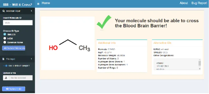
A aplicação web foi construída através do pacote Shiny para R. Este pacote permite a construção de uma UI (User Interface) gráfica, sem necessidade de conhecimentos prévios em desenvolvimento web, uma vez que o código em R é traduzido para JavaScript, CSS e HTML. O Shiny disponibiliza também várias widgets pré-definidas para construir as aplicações, assim como a possibilidade de adicionar pequenos trechos de código (i.e. JavaScript) para personalizar a interface. As aplicações elaboradas em Shiny baseiam-se no princípio de reactividade em programação, permitindo que as alterações feitas no input pelo utilizador se reflictam nos outputs devolvidos automaticamente, criando dependências entre os mesmos. A aplicação web desenvolvida permite aos utilizadores escolher o modelo a ser utilizado, inserir uma única molécula textualmente, onde SMILES, InChIs e nomes comuns são aceites ou inserir várias moléculas por meio de um ficheiro contendo SMILES ou InChIs. Existem dois tipos de output possíveis. Se apenas uma molécula é inserida, é mostrado o resultado para o modelo escolhido, assim como uma representação gráfica e informação adicional dessa mesma molécula. Se for inserido um ficheiro, o utilizador pode visualizar os vários resultados por meio de uma tabela interactiva. Nessa tabela pode explorar os resultados, seleccionar as moléculas que se encontram acima de um limite desejado e guardar os resultados.

De modo a garantir a manutenção e modularização da plataforma, foi utilizado o Docker de modo a separar cada componente (Aplicação Web, REST API e base de dados) no seu próprio “contentor” virtual com todas as dependências necessárias - facilitando, ao mesmo tempo, a comunicação entre estes componentes.

(9)

(10)

x

List of Figures

Figure 2.1 Drug Discovery, Design and Development. ... 3

Figure 2.2 Schematic Representation of Reactivity in Shiny.. ... 12

Figure 2.3 Virtual Machine vs Container Architecture. ... 13

Figure 2.4 Docker Containers Base Concepts and Commands. ... 14

Figure 2.5 Setting up a multi-container application with Docker-compose.. ... 15

Figure 3.1 Interaction Predictor Containerization Architecture ... 16

Figure 3.2 Interaction Predictor Platform Architecture. ... 17

Figure 3.3 The MVC Concept and the Interaction Predictor Platform Architecture.. ... 18

Figure 3.4 From Input to Output in the Shiny Web App. ... 23

Figure 4.1 Single Molecule Output - Prototype.. ... 24

Figure 4.2 Multiple Molecule Output - Prototype. ... 24

Figure 4.3 Prototype Design Architecture. ... 25

Figure 4.4 Available Resources in the REST API and their Results.. ... 26

Figure 4.5 REST API Model Resource Output Example.. ... 27

Figure 4.6 Interaction Predictor Homepage. . ... 28

Figure 4.7 Interaction Predictor Sidebar. ... 28

Figure 4.8 Interaction Predictor Target Tab.. ... 29

Figure 4.9 Interaction Predictor Molecule Tab Example.. ... 29

Figure 4.10 Interaction Predictor Single Output Schema.. ... 30

Figure 4.11 Interaction Predictor Single Output.. ... 30

Figure 4.12 From File to Output. ... 31

Figure 4.13 Multiple Output Interface. ... 32

Figure 4.14 Row selection and Download. ... 32

(12)

xii

List of Tables

(13)

xiii

Acronyms

AD: Applicability domain, 6

API: Application Programming Interface, v, vi, viii, xi, 2, 11, 16, 18, 19, 20, 21, 22, 23, 25, 26, 27, 35 CACTUS: CADD Group Chemoinformatics Tools and User Services, 9, 22, 25

CADD: Computer Aided Drug Design, 1, 4, 22, 35, 43 CSS: Cascading Style Sheets, viii, 11, 12, 23

GNU-GPL: GNU General Public License, 23 HTML: Hypertext Markup Language, viii, 11

HTTP: Hypertext Transfer Protocol, viii, 11, 20, 26, 43 IDE: Integrated development environment, 19, 22

InChI: IUPAC International Chemical Identifier, v, vi, 2, 9, 10, 19, 20, 21, 22, 24, 28, 29, 31, 33, 35, 41

LBVS: Ligand based virtual screening, 4 ML: Machine learning, x, 1, 2, 5, 8 MVC: Model-View-Controller, x, xi, 18

QSAR: Quantitative Structure Activity Relationship, v, vi, vii, viii, x, 1, 2, 4, 5, 6, 7, 9, 10, 28, 35, 36, 37, 38, 39, 40, 41

REST: Representational state transfer, v, vi, viii, x, xi, 2, 11, 16, 18, 19, 20, 21, 22, 23, 25, 26, 27, 35 SBVS: Structure based virtual screening, 4

SMILES: Simplified molecular-input line-entry system, v, vi, vii, viii, 2, 9, 10, 19, 20, 21, 22, 23, 24, 28, 29, 30, 31, 32, 33, 34, 35, 40, 41, 42

svg: Scalable Vector Graphics, 20, 21, 27, 29, 33 VM: Virtual machine, 13

(14)

1

1 Introduction

Computational methods and resources are increasingly essential in scientific research as biologic datasets grow in size and complexity [1]. In bioinformatics, most tools and software are provided by the research community, favouring open source development and knowledge dissemination in order to facilitate further scientific advancements [2], [3]. However, despite the release of various software by the community, there are challenges regarding distribution, delivery, integration and maintenance which hinder the scientific discovery process.

Bioinformatics resources are mostly the result of research, culminating in the publication of the method or results. As such, the dynamic in place tends toward the release of several short-lived pieces of software where portability, maintainability and accessibility are often disregarded beyond the end-goal of publication [4], [5]. Not only does this complicate attempts to reproduce results but also hinders further integration or use of said methods.

Added to the lack of accessibility, the implementations of bioinformatics resources can be very distinct and the use of said resources can be dependent on specifics of the development environment. These include hardware, operating system (OS) and software dependencies. For a researcher without a computation background, using these resources presents the added difficulty of attempting to replicate the required conditions to run the software as well as navigating sometimes convoluted interfaces. Also, attempting to integrate multiple methods adds the complexity of stringing together inputs through incompatible interfaces, adding to the time and effort needed to use these resources.

One such family of bioinformatic resources lacking in proper dissemination to its end users are Quantitative Structure Activity Relationship (QSAR) Machine Learning (ML) models, specifically in Computer Aided Drug Design (CADD). The Drug Discovery and Design process is a costly endeavour, requiring vast amounts of resources and spanning over several years [6]. There are strict requirements placed upon possible drug candidates and so a large portion of costs originate in failed compounds, unsuitable for continued development [7]. As such, it is crucial that effective methods be applied in order to guarantee potential in candidates. With the increasing volume of compound databases and available data, in silico tools have become invaluable in filtering through these massive amounts of information and also in predicting and optimizing therapeutic value [8].

Virtual Screening (VS) is one such tool, with the goal of finding promising active compounds from a large collection. There are two types of VS: structure-based (using information on the therapeutic target’s structure) and ligand-based (using information on known active ligands to the therapeutic target). An extremely useful ligand-based methodology is QSAR. QSAR analysis bridges the gap between structure and activity, based on the similarity principle. It is generally accepted that compounds with a similar structure are likely to show similar biological activity. While not absolute, this principle has produced consistent results. QSAR has been successfully applied both in VS as well as in optimization of compounds for desired properties like potency, solubility or low toxicity by elucidating the structural features present in molecules responsible for said desirable properties.

ML approaches to QSAR have automated and improved upon the process. Various ML algorithms such as Support Vector Machines, Random Forest and Neural Networks have been applied successfully in predicting target-ligand interactions and therapeutic qualities [9]. An important aspect of QSAR ML models and QSAR in general is the need to represent molecules, physical entities, in a way that properly encodes their structural information and is ‘understandable’ by the software. Different representations

(15)

2 such as SMILES, InChI or molecular fingerprints hold varying aspects and dimensions of structural information and are more or less apt for a particular method.

The increased volume and access to biological data, coupled with the growing number of freely accessible, open source tools for both cheminformatics and machine learning, facilitates the creation and optimization of QSAR ML models by researchers. However, the usefulness of the produced model is dependent on its actual use. In order for the model to be applied, optimized or integrated into an overarching methodology, it must be accessible to its core users: researchers. The present work intends to create a centralized platform where QSAR ML models predicting molecule interaction with various targets can be stored and used. Not only should it facilitate access to said models, it should also act as a standard interface for their use, removing model specific interface issues. Models should be accessible through a Shiny Web Application and through a REST API, allowing molecule input as SMILES or InChI, both widely used identifiers. Design-wise, the application’s setup should be portable and automated, simplifying both installation and use. Docker containers were used to ease the deployment process, as well as improve the application’s modularity and extensibility.

(16)

3

2 Concepts and Related Work

Drug Discovery Process

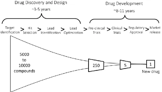
The drug discovery and development process consists of a series of steps starting from the study of a specific pathology and therapeutic target to the market release of the possibly resulting drug. The full process can take more than 12 years and often much longer to complete[6], and the costs can go above $1 billion, being a very expensive endeavour [10]. A simplified illustrative sequence is represented in Figure 2.1 (adapted from [11], [12])

The drug discovery process begins with the identification and validation of a therapeutic target (such as a receptor, enzyme or gene, among others) involved in a dysfunctional biological process pertaining a specific pathology [13]. The next step is hit selection: a large pool of compounds is evaluated using high-throughput screening (HTS) techniques. The active compounds, those with binding affinity to the target, are considered hits [14]. HTS allows screening of large collections of compounds for hits, using automated plate-based assays [15]. There are, however, limitations concerning low hit rates which derive from testing very large, unfiltered collections containing mostly inactive compounds (regarding the desired biological activity) [16], [17]. As such, costs increase with the number of tested compounds [18]. Once obtained, the most promising hits are considered leads which are not only active but also possess desired qualities such as low toxicity, patentability, synthetic accessibility, among other metrics [19]. These leads are then further optimized by medicinal chemistry, enhancing the necessary bio-pharmacological traits such as diminished toxicity and favourable absorption, distribution, metabolism, and excretion (ADME) properties [20]. Optimized leads move on to pre-clinical trials where, through animal testing, the toxicity analysis is performed detailing a projected safe dose range as well as information regarding compound distribution, organ-specific toxicity and metabolism. The often few resulting candidates then proceed to the clinical trial process, involving human testing.

Figure 2.1 Drug Discovery, Design and Development. Representative diagram showing the various stages from drug discovery

to drug development, complemented by average years for both discovery and development. Drug Discovery and Design encompass Target Identification, Hit Selection, Lead Identification and Lead Optimization. Drug Development includes Pre-clinical Trials, Clinical Trials, Regulatory Approval and Market Release. Also depicted is a visualization of the massive amounts of compounds that must be processed in order to produce a single potential drug, with a possibility of not even getting to the Market Release stage.

(17)

4 A successful product of drug discovery must not only present satisfying biologic activity with the target but also have the necessary properties regarding safety, kinetics, potency and other factors of therapeutic usefulness [13]. It’s due to these constraints that a large source of the costs associated with drug discovery are failed compounds, unsuitable for further development [7]. Given the costly nature of drug discovery and development, Computer Aided Drug Design (CADD) methods are used to complement the various stages, saving both time and resources and increasing success rates [8]. Virtual screening and QSAR methodologies are used to prioritize components for HTS in hit selection, improve hit-to-lead identification and enhance hit-to-lead optimization [21].

Virtual Screening

To increase effectiveness of hit selection, Virtual Screening (VS) methodologies are employed. While HTS attempts to test extremely large numbers of compounds in the most efficient way, VS attempts to rationalize and prioritize compound selection through pre-emptive filtering, increasing hit rates at a reduced cost [22]. Note that VS is not a substitute for in vitro and in vivo assays, but a complement [23]. There are two types of methods used in VS: structure-based [24], [25] and ligand-based [26], [27]. Essentially, structure-based methods are centred on complementarity between protein and ligand and require the 3D structure of the target, while ligand-based methods require information on molecules that bind to the target (ligands) and are based on the principle of similarity. Structure and Ligand based methods both hold importance in CADD, often used complementary in various stages of virtual screening pipelines [28].

For SBVS, target structure is determined experimentally through X-ray crystallography or NMR or, alternatively, predicted through homology modelling [29] (among other predictive methods). Using the determined 3D structure, molecular docking techniques attempt to predict the structure of the intermolecular complex formed between the target and tested molecules [30]. Precise information can be extracted from such methods, but the high complexity and computational cost are an issue.

LBVS methods do not require the 3D conformation of the target molecule, with knowledge of active ligands being used instead. Essentially, the similarity between candidate ligands and the known active compounds is used as a metric to predict desired biological activity. This approach is based on the structure-activity relationship (SAR) principle: there is a connection between structure and activity and, as such, structurally similar compounds tend to exhibit similar biological activity [31], [32]. LBVS approaches include scaffold hopping [33], pharmacophore modelling [34], Quantitative Structure Activity Relationship (QSAR) and also machine learning approaches to these methodologies. LBVS tends to require lower computational costs when compared to SBVS.

QSAR

Among the VS approaches, QSAR analysis is powerful method due to its favourable hit rate and fast throughput. QSAR is an in silico ligand-based method where molecular structure information is used to model and predict biological activity of interest. Traditionally, a pool of empirically characterized (labelled) molecules is used as a base of the QSAR model. The result was a simple linear classification model, which could then be used to classify a new compound. Essentially, QSAR models consist of an empirically established mathematical transformation from a compounds’ structural properties to its biological activity [35]. QSAR is based on the aforementioned similarity principle. This principle states

(18)

5 that structurally similar molecules tend to exhibit similar biological activities [31], [32]. While generally valid, minor modifications of functional groups can abruptly alter a compounds activity (despite high structural similarity) in what are known as activity cliffs. The presence of activity cliffs depends on the dataset and on the descriptors used to describe molecules and must be taken into account as it can lead to the failure or invalidation of QSAR models [36].

The rise of ML approaches to the drug discovery process has been applied to upgrade the traditional QSAR methodologies. These approaches use pattern recognition algorithms to automate the SAR and extrapolate pharmacologic properties of new compounds. Using QSAR ML methods, researchers can predict interactions with target molecules (hit detection) as well as optimize lead compounds by predicting what chemical modifications may result in favourable physiochemical properties [9]. The general process to create a QSAR machine learning model consists of several steps involving various techniques, from cheminformatics to machine learning. Firstly, each compounds’ structural information must be translated in a computable manner to be used as input for the model (feature vector). This information is often encoded in descriptors (molecular properties) or fingerprints (bit strings representing structural features and descriptors). Through feature selection methodologies, the most relevant information is chosen as a base for the learning phase of the model. Through the learning phase, the optimal mapping between the feature vectors and the relevant biologic response is discovered. Finally, the model’s performance is evaluated by metrics such as sensitivity, specificity, precision and recall. The elaboration of a successful QSAR ML model is highly dependent upon the composition of the dataset used for training and validation [37] as well as the choice of a relevant feature vectors and of the molecular structure representation [38].

2.3.1 ML Models

Generally speaking, ML models can be divided into supervised and unsupervised learning [39]. In supervised learning each instance in the training dataset is assigned a label, which the model should (after the learning phase) be capable of predicting in new instances. Whereas in unsupervised learning the training dataset is not labelled, and the model learns the underlying patterns in the dataset. The particular case of semi-supervised learning is also an option, where only some instances are labelled, in order to increase accuracy in small unbalanced datasets [40]. Supervised algorithms include multiple regression analysis [41], k-nearest neighbour [42], naïve bayes [43], random forest [44], neural networks [45] and Support Vector Machines (SVM) [42]. Unsupervised algorithms include k-means clustering [46], hierarchical clustering [46], Principal Component Analysis (PCA) [47] and independent component analysis [48].

These various techniques allow the exploration of the often complex and nonlinear SAR relationships between compounds. Beyond simply predicting interaction, potency or toxicity, ML models are also used to pinpoint the descriptors most relevant to a desired endpoint. With a plethora of available descriptors, issues regarding correlation, redundancy and high dimensionality diminish the quality of a finalized model. A problem aggravated by the often superior numbers of descriptors to the number of instances used to train the model [37]. Several ML techniques are used to tackle this matter, both through feature reduction (combine sets of features into statistically independent new components) and feature selection (selecting the minimum number of relevant features with the highest impact on model quality).

(19)

6

2.3.2 Measuring Similarity

At the core of QSAR models is similarity and it must be quantified. Several metrics exist to this end. Structural similarity is often evaluated using the Tanimoto coefficient between two feature vectors (i.e. fingerprints) [49]. This coefficient computes a similarity score according to the fraction of shared bits, meaning that a pair of molecules with a high Tanimoto coefficient are similar (though it offers no information specifically as to why they are similar). This coefficient can also be extended to 3D fingerprint comparison [50], with the alternative being pharmacophore similarity.

2.3.3 Applicability Domain

An important step in developing a successful QSAR model is identifying and establishing the Applicability Domain (AD) [51], [52]. AD refers to the physico-chemical, structural or biological space where the model is considered exploitable and its predictions reliable [53]. Without an AD, a model could technically predict the activity of any compound, even if said compound had a completely different structure to those in the model’s training dataset. Predictions made for compounds outside this domain hold no real predictive value and should be considered data extrapolation.

(20)

7

Chemical Representation

2.4.1 Representing Molecular Structure

As previously mentioned, the adequate representation of molecular structure is crucial in guaranteeing a quality QSAR model [38]. Both molecular descriptors and fingerprints are used to this end.

2.4.1.1 Descriptors

Descriptors are numerical features of a molecule which capture its structural characteristics and chemical properties. Descriptors can be classified according to dimensionality (1 dimensional through 4 dimensional) [54] or the nature of the encoded information (constitutional, topological, geometrical, thermodynamic and electronic) [55]. 1D descriptors are constitutional values based on the molecular formula and chemical graphs which include atom counts, molecular weight, fragment counts or functional group counts. While simple to compute, these descriptors often do not hold enough information to differentiate between compounds and must be coupled with higher dimensionality descriptors [56]. 2D descriptors are based on structural topology and represent atom connectivity in molecules, being some of the most commonly used in QSAR. These include topological indices, molecular size, shape and branching [56]. 3D descriptors are based on 3D coordinate representation of the atoms in a molecule and are sensitive to structural variation. While presenting a high information content, the related computing costs related to alignment are also high. 4D descriptors build upon 3D descriptors by considering multiple structural conformations [57].

2.4.1.2 Molecular Fingerprints

Chemical Fingerprints are fixed-length bit strings encoding a molecule where each bit represents the presence (1) or absence (0) of a feature (either on its own or in conjunction with other bits). These features can account for molecular descriptors, structural fragments or different types of pharmacophores. Several types of fingerprints have been developed, from simple representations of occurrence of functional groups to more complex multi-point 3D pharmacophore arrangements. 2D fingerprints use the 2D molecular graph and 3D fingerprints store 3D information as well.

There are several types of fingerprints, distinguished by the method used to encode the molecule into a bit string, as listed below (adapted from [58]):

• Topological fingerprints (i.e. Daylight [59], atom pairs [60]) • Structural keys (i.e. MACCS [61], BCI [62])

• Circular fingerprints (i.e. Molprint2D [63], ECFP, ECFP [64])

• Pharmacophore fingerprints (i.e. CAT descriptors [65], 3pt [66], [67] and 4pt [68] 3D fingerprints)

• Hybrid fingerprints (i.e. Unity 2D [69])

• Protein-ligand interaction fingerprints (i.e. SMIfp [70], SIFFt [71])

Substructure keys-based fingerprints encode the presence of certain substructures of features from a given set of structural keys. This means that the usefulness of such fingerprints is dependent on whether or not the structural keys are heavily present in the compounds. Examples of such fingerprints include: MACCS [61], PubChem fingerprint [72], BCI fingerprints [73], TGD [74] and TGT fingerprints.

(21)

8 In topological fingerprints all fragments of the molecule are analysed, following a path up to a certain number of bonds. The hashed version of all of these paths constitutes the fingerprint. The length of the fingerprint is adjustable by altering the maximum number of bonds for the paths. The Daylight [2] fingerprint is the most commonly used and is often used in substructure searching and filtering. Circular fingerprints are similar to topological fingerprints. Starting from each atom, the neighbouring environment is iteratively recorded up to a pre-determined radius. While unsuitable for substructure searching (as the focus is not on fragments but on their environment), this type of fingerprints is widely used in similarity searching. Examples include Molprint2D [75], [76] and ECFP. Extended-Connectivity Fingerprints (ECFPs) represent circular atom neighbourhoods and were specifically designed for structure-activity modelling [64]. They are based on the Morgan algorithm which assigns unique sequential atom numbering to any given molecule. Both circular and topological fingerprints are hashed, which means each bit cannot be traced back to the original feature.

While perhaps counter-intuitive, higher complexity fingerprints (3D) do not necessarily equal better performance in predictive models or virtual screening experiments [77]. 2D fingerprints show superior results, are easier and faster to calculate and are readily available through free, open-source toolkits such as RDKIT [78], OpenBabel [79] or CDK [80], [81]. They have also been extensively used in building predictive ML models for drug discovery, with endpoint such as target potency [82], [83], genotoxicity [84] and other ligand-based similarity analysis methodologies [58].

(22)

9

2.4.2 Identifying a Molecule - Chemical Identifiers

A chemical identifier is essentially a label denoting a chemical substance. These labels provide a way of distinguishing, comparing, storing and analysing compounds. This requires reproducible notations from the simplest atom to intricate chemical structures. An identifier is considered non-ambiguous if it identifies a single possible structure, and unique if said structure can only be represented by that identifier. With the increasing automation on chemical data processing, it is paramount that these identifiers hold relevant physical and structural information, are designed to be read by software applications and are consistently applied throughout available resources. Specifically in QSAR studies, inconsistencies between the actual structural information of a molecule and the chosen identifier (the computer readable structure) have a high impact in model quality and predictive ability [85]. Discrepancies between the actual stereochemistry of compounds and the stereochemistry encoded in the identifier are an example of such issues.

Chemical Identifiers can be either systematic or non-systematic. Systematic identifiers are algorithmically defined through the chemical structure of the compounds [86]. These include linear notations such as IUPAC [87], SMILES [88], and InChIs [89]. Conversely, non-systematic identifiers are assigned to a compound when registered to a database. These include generic names, chemical abstracts service (CAS) registry numbers, and database specific identifiers such as PubChem CIDs, ChemSpider IDs, and ChEMBL IDs. Resolving Chemical identifiers into alternative ones can be achieved through lookup and translation approaches. Lookup takes advantage of databases connecting various identifiers to each compound. Services such as CACTUS, UniChem and PubChem Identifier Exchange cross-reference various databases to find alternative identifiers. The translation approach involves algorithmically converting a representation of a compound into another of the same compound. RDKit and OpenBabel are open-source toolkits with this functionality.

Linear notations represent chemical structures as a linear string of symbolic characters which can be interpreted by systematic rule sets. Their popular use derives from being compact, reasonably human readable and more effective for computer processing, especially when handling large amounts of data. They are used for storing, representing, communicating and comparing similarity of compounds. The most widely used linear notations are the SMILES (Simplified Molecular Input Line Entry System) developed by Weininger [88] and Daylight Chemical Information Systems [59], and IUPAC’s InChI (International Chemistry Identifier) [89]. Examples of other line notations include the Wiswesser Line-Formula Notation (WLN) [90], Sybyl Line Notation (SLN) [91] , Representation of structure diagram arranged linearly (ROSDAL) [92] and Modular Chemical Descriptor Language (MCDL) [93].

2.4.2.1 SMILES

The Simplified Molecular Input Line Entry System (SMILES) is a linear notation of a chemical’s structure’s molecular graph created by David Weininger and later developed by Daylight Chemical Information Systems. The SMILES format is widely used, describing chemical structure in a compact, intuitive and overall human-readable manner, using a small amount of natural grammar rules. Beyond its intuitive design, its nature as a linear notation makes it optimized for computer processing.

The SMILES notation is based on the valence model of chemistry, where a molecule is represented as a mathematical graph: nodes are atoms and edges are semi-rigid bonds respective valence bond theory. While this model has proven a useful approximation of atom behaviour, it does not accurately describe the underlying quantum-mechanical dynamic of subatomic particles. It is of note that SMILES strings

(23)

10 do not specify all types of stereochemistry: helices, mechanical interferences or the shape of a protein after folding are not represented. Nevertheless, SMILES can specify the cis/trans configuration around a double bond and the chiral configuration of specific atoms. The SMILES notation is non-ambiguous but not unique: a molecule can be represented by various SMILES. To alleviate this issue, there are Canonical SMILES representations, where the same SMILES is always produced for a said molecule. However, it is still not advised to use Canonical SMILES as universal identifiers (i.e. for a database), with InChI representation being recommended. Beyond its widespread use as a chemical identifier, SMILES-based descriptors have been used in QSAR modelling [94]–[96].

2.4.2.2 InChI

InChI is a non-proprietary, open-source, chemical identifier originally developed by IUPAC [87], [89]. InChI algorithm combines a normalisation procedure, a canonicalization algorithm, and a layered structure. Due to its open-source nature, the same implementation as the official InChI algorithm can be found in several cheminformatics toolkits such as RDKit [78] and OpenBabel [79]. Unlike SMILES, InChI was not developed with human readability in mind, but instead with a focus on machine processing. Another distinction between the two notations is the is consistency of its generation algorithm, unlike the various implementations of the SMILES algorithm [92], [97]. The main features of InChI are as follows: (Adapted from [89])

• Structure-based approach; • Unique identifier

• Non-proprietary

• Applicable to the entire domain of classic organic chemistry and, to a significant extent, to inorganic chemistry;

• Ability to generate the same InChI for structures drawn under different conventions; • Hierarchical layering encoding of molecular structure, allowing for various levels of detail; • Ability to produce an identifier with standardized granularity.

InChI encodes structural features in hierarchical layers. Each layer is a distinct class of structural information which are ordered sequentially, increasing in detail. There are six major InChI layers: Main, Charge, Stereochemical, Isotopic, FixedH and the Reconnected layer. The main layer specifies chemical formula and must be present, with the remaining layers being added if the equivalent information is provided. The layered nature of InChI allows the user to represent a molecule with varying degrees of detail. Consequently, a single molecule can be represented by multiple InChIs. To improve standardization, the Standard InChI is produced with fixed options, guaranteeing uniqueness. This standard distinguishes connectivity, stereochemistry, and isotopic composition.

The size of an InChI string increases with the size of the corresponding chemical structure, resulting in very long identifiers, which is unoptimized for indexing operations. The InChIKey is a fixed-length 27-character hashed string of upper-case 27-characters derived from InChI [89]; far more convenient for searches and database indexing. InChIKeys are divided in three blocks separated by hyphens: the first 14 characters encode the main layer, the following 10 characters encode other structural features such as stereochemistry, and the final character encodes protonation state. The hashing nature of InChIKeys signifies that there is a possibility of collision: two molecules generate the same InChIKey. However, the actual collision rate is very low [98].

(24)

11

REST Services, Web Applications and Containerization

The implemented platform involves both a Web Application developed using Shiny and a REST service to provide the user with access to the machine learning models. Both services and additional functionalities are bundled up in the virtualization software Docker. The following section attempts to clarify these concepts, as a base for understanding the chosen implementations.

2.5.1 REST Service

REST (Representational State Transfer) is an architectural style defined by a set of design principles for building web services. These services allow access and manipulation of resources through a uniform interface and set of stateless operations. A client program uses APIs (Application Programming Interfaces) to communicate with the web service, handling listening and responding to client requests. A web service with a REST API is considered a RESTful service.

A resource is a generic concept which refers to something which can be uniquely identified and has at least one representation. A resource can be a file, a web page or media, among others. Resources must be identified by at least one URI (Unique Resource Identifier). URIs can be either a URL (Uniform Resource Locator) or an URN (Uniform Resource Name). URN defines a unique name to a resource, while URL defines a means to obtain the referenced resource. Not only should any resource be identified by a URI but should also be directly accessible through it.

REST uses standard HTTP operations to assure a uniform interface. Such operations include: PUT (create/update resource), GET (retrieve resource representation), POST (modify resource state) and DELETE (remove resource). Since these HTTP operations mean the same across the web, the request is separate from the resource on which it is applied or the client who made said request. Ensuring this uniform interface means that a) performing an operation has the same effect whether it was performed once or multiple times and b) operations on a resource do not change the server state, independently of the number of times they performed.

In a RESTful service, the client application requests should contain all necessary information for the server to process and fulfil said request. This means the interactions are stateless. The client application handles necessary context information, removing the burden from the server to track client information, increasing scalability.

2.5.2 Shiny

Shiny is an open-source R package allowing the creation of interactive web applications. It is designed so that developers who wish to create an application needn’t have a background in web development. Both back end and front end are programmed in R and shiny handles the creation of the dynamic web page.

STRUCTURE

A shiny app is divided in two components: the UI object and the server function. For this project, both objects were defined in separate files: ui.R and server.R. It is also possible to have a single app.R file where both components are defined and passed as arguments to a shinyApp() function but this makes the code less manageable. The ui object is defined using shiny specific functions which are then translated to HTML, CSS and JavaScript, creating the dynamic web page. The basic UI structure begins

(25)

12 with a page defining function, then page-component defining functions (i.e. header, sidebar and body in the case of a dashboard template) and finally the input widgets (i.e. text or files) and outputs (i.e. plots, tables or text). The server function handles server-side calculations, data manipulation and output rendering. All inputs are stored in an input object and can be accessed using the corresponding id in a R list-like syntax. If the application contains a text input widget with the id “example_textinput” its value can be accessed through input$example_textinput. The same happens with the output object: if a plot is defined in the server function (using a render function) with the id “example_plot” it can be accessed through output$example_plot.

REACTIVITY

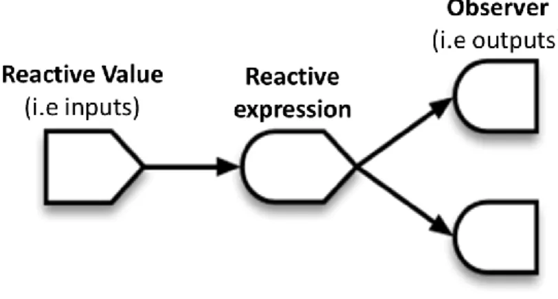
Given its interactive nature, Shiny uses reactivity to guarantee that changes made to input by the user are reflected in the output. Inputs are considered reactive values and are updated when altered. These reactive values can then be called and handled by reactive expressions, which can in turn be accessed by other reactive expressions. The crucial detail to reactive expressions is that every reactive value that was read or reactive expression that was called is considered a dependency, and if any of those dependencies are invalidated (a change occurred) then the expression must re-execute to update its own value. Essentially, changing any input will automatically cause any reactive expression dependent on that input to re-execute. A schematic representation of reactivity is shown in Figure 2.2, adapted from [99].

This reactivity can be modulated by the developer, using types of reactive expressions such as eventReactive() which assure an expression will only re-execute when a specific event occurs (such as a button click) and its dependencies have changed.

CUSTOMIZATION

Shiny comes with a variety of widgets and graphical elements to build the application. However, these can be expanded upon using user-created packages such as shinyWidgets, shinydashboardPlus or shinyalert which add new or improved content as well as extra functionality. Furthermore, developers with knowledge of CSS can link to an external stylesheet to customize every element of the web app. This file, along with any local files used in the app (such as images, data files, etc) are stored in a predefined /www folder inside the main app directory.

Figure 2.2 Schematic Representation of Reactivity in Shiny. Reactivity in Shiny is achieved by integrating three types of

reactive elements: reactive values, reactive expressions and observers. Reactive values are objects such as inputs or other defined-as-reactive variables which, when invalidated (i.e. a change in input) communicate that invalidation to any reactive expressions or observers dependent on themselves. A reactive expression is any expression based on some reactive value which returns value and will update when its dependencies are invalidated. Observers are objects such as outputs or defined-as-observer expressions which are dependent on reactive values and will re-evaluate when its dependencies are invalidated and, most notably, do not return a value and are, instead, used for their ‘side-effects’ such as the creation of a table, plot or UI element.

(26)

13

2.5.3 Containers

Computation has become an integral part of scientific research and with increasing amounts of bioinformatic software being produced, the subject of deployment and reproducibility grows in importance. Independently of the usefulness of the software, it must properly reach and be used by its end user. Researchers originating relevant and powerful tools may see the reach of their work hampered by challenges in result reproducibility. With computer environments constantly changing, guaranteeing a piece of software will run in the same manner as it did in the development environment presents a challenge. Common issues include large amounts of dependencies (requiring the recreation of the development environment), dependency invalidation (through updates, deprecated features, etc) and difficulties in integrating pre-existing tools in novel workflows [100]–[102].

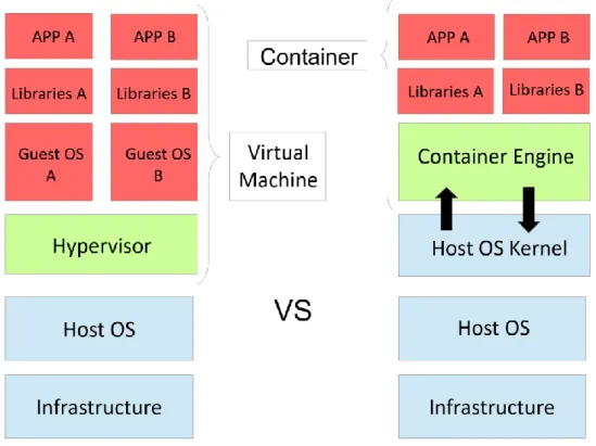
Virtualization technologies such as Virtual Machines (VM) and containers attempt to tackle these challenges by isolating both an application and its dependencies in a self-contained unit to run in whatever environment the user may prefer. Despite the having the same goal, VM and containers use a distinct architectural approach: VMs use hardware virtualization through a dedicated OS while containers provide OS-level virtualization by using the host’s system kernel across all containers (Figure 2.3). The container’s architecture makes them more lightweight with equal or even increased performance when compared to VMs [103]. Containers are also designed towards modularization and combining multiple services which is not as feasible with the heavy VMs, in the case that each component must run inside its own VM. However, as containers communicate directly with the host’s kernel, security concerns can be relevant.

Figure 2.3 Virtual Machine vs Container Architecture. Virtual Machines use hardware-level virtualization: the Hypervisor

handles the creation and maintenance of a complete virtual OS on top of a host machine OS, each with its own libraries and software, thus achieving virtualization. On the other hand, containers take advantage of the host’s OS kernel and use it across containers. The container engine handles the creation and maintenance of these containers, each with their own libraries and software.

(27)

14 Docker is an open source, Linux container-based tool for application packaging and deployment. Docker is designed to host one service per container and then allow communication between containers to build up to a multi component application. If, for example, a web application requires a database, both the database and the application are built inside their own containers (with their own dependencies) with ways of communicating between them.

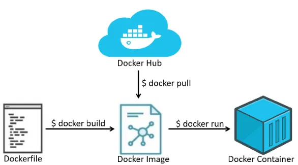
Containerization in Docker is focused around Docker images (Figure 2.4). These images are read-only templates containing all necessary dependencies, files and scripts necessary for the application, as well as what to run when the container is launched. These images are built using Dockerfiles: plain text files with a simple script composed of various instructions, such as which base image to start from, dependencies to install, environment variables to set, ports to open and commands to run on launch. When an image is run to create a container, Docker adds a read-write file system over the image, creates a network for communication between the host and the container, assigns an IP address to the container and executes the process specified to run on start up in the image. Essentially, a container is a running instance of an image. Docker Hub is a free centralized repository of pre-built images available for download and use. These images can be directly accessed through Docker as full applications or as a base for another image. User created images can also be easily stored and published in the Docker Hub.

Dockerfiles’ simple syntax documents necessary dependencies for running the application in a human readable way, as well allowing easy image customization by direct editing of the script. The Dockerfile can also be shared and stored as an alternative to image sharing. A Docker image holds all necessary software already installed and configurated, so the user needs only install Docker software to access it. Software versions can be defined in the Dockerfile and changes can be tracked in the image itself, facilitating management of deprecated software. Docker Hub also holds the various versions of images, allowing the user to choose which to use. Essentially, Docker’s strengths lie in its portability, version control and accessibility.

Figure 2.4 Docker Containers Base Concepts and Commands. At the core of Docker’s containerization strategy are Docker

Images: these can be understood as snapshots of a fully fledged container, with all dependencies, software and files present. Docker Images are built (not exclusively) through Dockerfiles. These files are essentially a series of instructions to build the environment; here, the source image is defined, ports are exposed, files are copied into the container filesystem and dependencies are listed for installation. The docker build command uses a Dockerfile to build a Docker Image. Docker Images can also be pulled directly from the Docker Hub, a central repository from Docker with a variety of images, with the command Docker pull. Finally, containers are running instances of images, an operational environment. The command docker run initiates a container from an image.

(28)

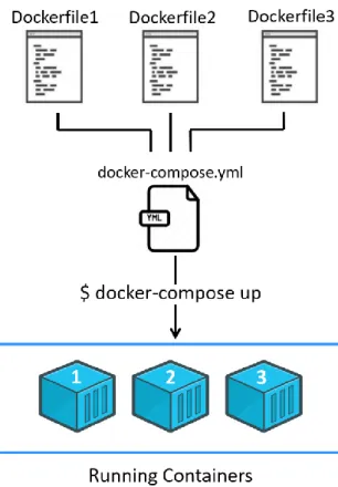
15 Docker Compose is a tool used to set up multi-container applications so they can run together in an isolated environment. A YAML file is used to set up each container as a service (how to build, ports to expose, dependencies between services, volumes to build, etc) and connect them accordingly. With a single command (docker-compose up), all containers called in the .yml file are started and connected between them (Figure 2.5). As Docker is built around one service per container, this approach allows a simple interface to connect multiple containers adding up to a fully-fledged application.

Figure 2.5 Setting up a multi-container application with Docker-compose. While Docker already allows the linking of

containers, Docker-compose simplifies this and standardizes the inter-container connections, allowing commands to be applied to all containers in the application. To set-up connected containers, a docker-compose.yml file defines each container as a service, instructing how to build each one in succession from their respective Dockerfiles, connecting them in a shared network and setting up dependencies between them. The command docker-compose up reads the docker-compose.yml file and builds the images for each container and gets them running in tandem.

(29)

16

3 Materials and Methods

Platform Architecture

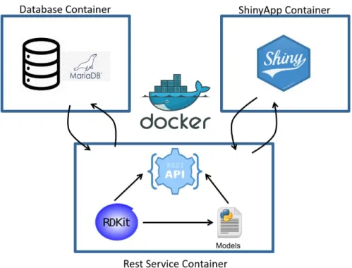
The application is divided into 3 essential components, each compartmentalized in their own Docker container: REST service, Shiny Web App and Database (Figure 3.1). The application is running in a server with Docker and Docker-compose installed. All other service-specific software is installed in each container.

Each container holds the necessary files, libraries and resources necessary to run their corresponding service. The docker-compose.yml file instructs the three separate containers to run in tandem, facilitating inter-container communication. Each container is considered a service: being given a container name, how it should be built (either through a Dockerfile or a base image from Docker Hub), which ports to expose, volumes to build (if necessary), dependencies on other services (the Database must be setup before the REST service which in turn must be setup before the Shiny Web App) and other service specific variables. Essentially, the models are made available to the user through the REST API and the Shiny Web Application. The REST API handles the running of the models, molecule processing and necessary calculations using RDKIT (i.e. fingerprint and SVG generation) and database communication. The Shiny Web App accesses the models through calls to the REST API, rendering the output in a user-oriented graphical interface. The overall architecture of the platform is represented in Figure 3.2.

Figure 3.1 Interaction Predictor Containerization Architecture. The platform is divided in three separate containers, linked

through docker-compose. The REST Service holds the necessary software and dependencies for running the models such as RDKIT and the packages for building the REST API. This container communicates directly with the Database container. This one contains a running implementation of MariaDB, for result storage. The ShinyApp container holds the Web Application, having, most importantly, Shiny and its dependencies installed. This container communication with the REST API and not with the Database.

(30)

17

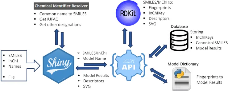
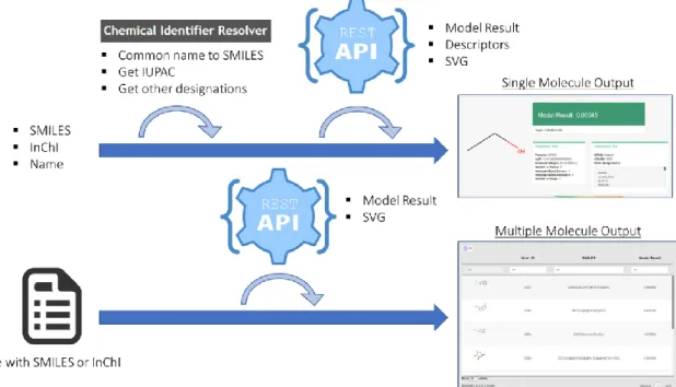
Figure 3.2 Interaction Predictor Platform Architecture. Input enters the Shiny Web App either as a single identifier

(SMILES/InChI/Common Name) or a file with multiple (SMILES/InChI). The Web App resolves Common Names into SMILES through the CACTUS Identifier Resolver API, and also retrieves the IUPAC and other designations of the molecule (if single input). The Web App then requests the REST API Model resource, sending the chosen model and identifiers. The REST API processes the identifiers with RDKIT, converting to InChIKey to check the Database for stored results. If none are present, the model dictionary is accessed, the identifiers are converted to molecular fingerprints (using RDKIT) and the appropriate model is run, and result collected and stored in the database. The REST API then return the results to the Web App. The REST API also returns a svg representation of the molecule as well a series of descriptors (each returned by their appropriate resources). Finally, the Web Application renders the outputs to the user. Note that the REST API is also directly accessible to the user.

(31)

18

3.1.2 MVC and Platform Architecture

The Model-View-Controller (MVC) in an architectural pattern in which an application’s logic is divided into three interconnected main components: Model, View and Controller. Each of these components are responsible for specific functions within the application.

▪ Model - corresponds to the data-related logic of the application, independent of the user interface (View). Processing, calculations and information retrieval are handled by the Model. ▪ View - holds the UI-logic of the application: presentation of the Model in a particular format. ▪ Controller - the interface between the Model and View components. It is responsible for

accepting input, manipulate and update the Model accordingly and instruct the View how to render output.

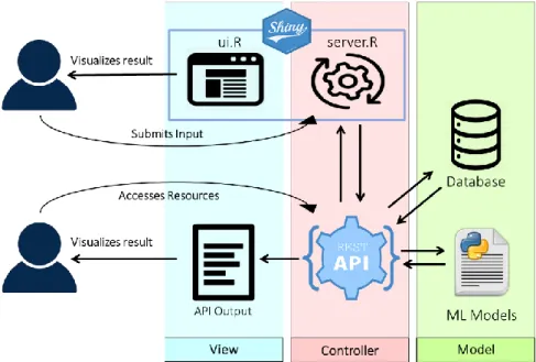
The MVC design intends to modularize the application in a way that improves maintainability, facilitates testing and encourages structured and clear code. Unlike the prototype, the final application was constructed with the MVC design in mind. In this implementation (Figure 3.3), the Model component is comprised of the actual machine learning model which returns the results and the database storing these results. The Controller houses both the REST API and the server.R component of the Shiny Web App. In the server component, the user input is sent to the API, where it is sent to the Model (models and database) and the retrieved results are sent back to the server component for transformation into output or to the user if the request was made directly to the REST API. In this MVC implementation there are, as such, two possible views: the Shiny Web App ui.R object which shows the output rendered in server.R and the JSON like return values from direct calls to the REST API.

Due to the implementation of Shiny and its underlying architecture, the MVC concepts are not fully applicable in practical terms. However, its core design ideas were used as the foundation for the platform’s modularized organization strategy.

Figure 3.3 The MVC Concept and the Interaction Predictor Platform Architecture. From the Model-View-Controller

perspective, there are two Views available to the user: the UI of the Shiny Web App (defined in ui.R) and the direct output of the REST API. The Controller is comprised of the server component of the Web App which receives the identifiers and model choice from the user (inputs) and requests the results from the REST API, the second component, which coordinates the processing of the identifiers and model into results and other resources. The Model includes both the machine learning models which yield the results as well as the database where they are stored.

(32)

19

REST Service

The base image for the container holding the REST API is a bootstrapped Anaconda 3 installation pulled from the Docker Hub: https://hub.docker.com/r/continuumio/anaconda3. This was necessary as RDKIT is an integral toolkit to the functioning of the application, and the installation through the anaconda package manager was the most stable and successful option. This does have the downside of increasing the size of the resulting image considerably.

The REST API was written in Python and developed in the IDLE IDE. Python is a high level, object oriented, cross platform and open-source general purpose language. Its clear syntax helps with code readability and maintainability. It is used for web and software development, scientific computing, among others. Boasting an active community, the The Python Package Index (PyPI) holds many varied user-created packages which expand upon the language’s functionality.

Used packages:

▪ Flask 1.0.2 for the micro web framework [104]

▪ Flask-RESTful 0.3.6 to expand upon flask to create a REST API [105] ▪ mysql.connector 8.0.16 to handle database communication [106]

▪ rdkit 2019.03.2.0 to handle molecule identifiers, descriptors and fingerprints [78] ▪ pandas 0.24.2 for dataframe handling

▪ pickle 4.0 to read model files

▪ rpy2 2.9.1 to run snippets of R code in Python [107]

3.2.1 Handling Identifiers and Structural Representations - RDKIT

The platform manages various chemical identifiers and structural representations and RDKIT was used as the main resource to handle the necessary cheminformatics functions on these identifiers and representations. RDKit [78] is an open source collection of cheminformatics and machine-learning software written in C++ and Python. Features of this toolkit include:

• Reading and writing molecules; • Modifying molecules

• Drawing molecules • Substructure matching • Descriptor generation

• Fingerprint generation and similarity

In RDKit, molecules can be read from a variety of sources such as SMILES, InChI and files containing molecular structure like MOL and SDF formats. A variety of functions read these sources and create a Mol object (RDKits’ representation of a molecule) which is the foundation for a large portion of the cheminformatics operations available in RDKIT. From the Mol object, the molecule can be written in a variety of formats including SMILES, InChI, InChIKey, JSON and MOL files. This read/write implementation means that it can be used as an identifier resolver, converting between molecule representations. Using the structural information of each molecule, the toolkit can also create images in various formats including SVG. The Mol object has methods in place to inspect, return and modify its constituents such as atoms, bonds, rings, among others. One of the functionalities of RDKit is substructure matching between Mol objects. This can be used for molecule filtering as well as for substructure-based transformations like substructure replacement, addition and deletion. From the Mol