Stefano Beretta
1, Mauro Castelli
2, Ivo Gonc¸alves
2, Ivan Merelli
3and Daniele Ramazzotti
41DISCo, Universit´a degli Studi di Milano Bicocca, 20126 Milano, Italy 2NOVA IMS, Universidade Nova de Lisboa, 1070-312 Lisboa, Portugal 3Ist. di Tecnologie Biomediche, Consiglio Nazionale delle Ricerche, Segrate, Italy
4Department of Pathology, Stanford University, Stanford, U.S.A.
Keywords: Bayesian Graphical Models, Breast Cancer, Genetic Algorithms, Network Inference.
Abstract: Gene and protein networks are very important to model complex large-scale systems in molecular biology. Inferring or reverseengineering such networks can be defined as the process of identifying gene/protein inter-actions from experimental data through computational analysis. However, this task is typically complicated by the enormously large scale of the unknowns in a rather small sample size. Furthermore, when the goal is to study causal relationships within the network, tools capable of overcoming the limitations of correlation networks are required. In this work, we make use of Bayesian Graphical Models to attach this problem and, specifically, we perform a comparative study of different state-of-the-art heuristics, analyzing their perfor-mance in inferring the structure of the Bayesian Network from breast cancer data.
1 INTRODUCTION
Molecular networks are essential for every biologi-cal process, since genes and proteins are able to carry out their function only in precisely regulated path-ways. For this reason, data-driven learning of regula-tory connections in molecular networks has long been a key topic in computational biology (Bansal et al., 2007). The general problem is to infer, or reverse-engineer, from gene or protein expression data, the regulatory interactions among these biological enti-ties using computational algorithms.
In this context, despite correlation networks are widely used for gene expression and proteomic data analysis, it is known that correlations not only con-found direct and indirect associations, but also pro-vide no means to distinguish between cause and ef-fect. For causal analysis the inference of a directed graphical model is typically required. However, this task is rather difficult due to multiple theoretical and practical reasons, among which, but not limited to, the course of dimensionality (Pearl, 2003).
Therefore, causal analysis requires tools capable of overcoming the limitations of correlation networks: much of the work in this area has focused on Bayesian Networks (Pearl, 2003) or related regression models,
such as systems of recursive equations or influence di-agrams. All these models describe causal relations by an underlying directed acyclic graph (DAG). Never-theless, it remains unclear whether causal, rather than merely correlational, relationships in molecular net-works can be inferred in complex biological settings. Moreover, the problem is typically complicated by the enormously large scale of the unknowns in a rather small sample size. Furthermore, data is prone to ex-perimental defects and noisy readings, while many other biases can compromise the quality of the results. These complexities call for a heavy involvement of powerful mathematical models which play an in-creasingly important role in this research area (Kabir et al., 2010). In order to assess the ability of dif-ferent tools to learn causal networks, the Dialogue for Reverse Engineering Assessment and Methods (DREAM) project has run several challenges focused on network inferences (Stolovitzky et al., 2007). In particular, we focused on (sub)-challenge 8.1 con-cerning Human Protein Networks (HPN) in cancer cell lines, which is about the inference of causal sig-nalling pathways using time-course data with pertur-bations on network nodes. This sub-challenge was split into two independent parts, concerning Breast Cancer proteomic data and in silico data.
Beretta, S., Castelli, M., Gonçalves, I., Merelli, I. and Ramazzotti, D.
Combining Bayesian Approaches and Evolutionary Techniques for the Inference of Breast Cancer Networks. DOI: 10.5220/0006064102170224
Different types of models, such as directed graphs, Boolean networks (Akutsu et al., 1999), Bayesian Graphical Models (Zou and Conzen, 2005), and var-ious differential models have been used to describe gene regulations at various levels of detail and com-plexity. The choice of the model is often determined by how much information it tries to capture, taking into account that the more information a model at-tempts to infer, the more parameters are needed to learn it, and the more complex the overall approach becomes. Specifically, researchers have paid great at-tention to Bayesian Networks, which can compactly model dependency relationships between variables relying on probabilistic measures. Since gene expres-sion experiments are subject to many measurement er-rors, the use of statistical methods is expected to be effective for extracting useful information from such noisy data. Friedman et al. (Friedman et al., 2000) proposed both discrete and continuous Bayesian net-work models relying on linear regression for infer-ring gene networks. Imoto et al. (Imoto et al., 2001) succeeded in employing non-parametric regressions for capturing even non-linear relationships between genes.
In this work, we perform a comparative study of different heuristics at the state-of-the-art to perform the task of inferring the structure of a Bayesian net-work from breast cancer data. The paper is struc-tured as follows: Section 2 provides a background of the biological problem under exam; Section 3 gives a formal definition of the problem addressed in this study, along with a description of the different compu-tational and statistical machineries that we are adopt-ing, and of the input data. Afterwards, the results of the described methods on real and simulated data are presented and discussed in Section 4. Section 5 con-cludes the paper and suggests avenues for future re-search.
2 BIOLOGICAL BACKGROUND
Many biological processes are carried out by inter-actions between proteins, RNA, and DNA. Cells re-spond to their environment by activating signalling networks that trigger processes such as growth, sur-vival, apoptosis (programmed cell death), and migra-tion. Post-translational modifications, notably phos-phorylation, play a key role in these signalling events. In cancer cells, signalling networks frequently be-come compromised, leading to abnormal behaviours and responses to external stimuli. Endogenous sig-nal transduction in cancer cells is systematically dis-turbed to redirect the cellular decisions from
differen-tiation and apoptosis to proliferation and, later, inva-sion. Cancer cells acquire their malignancy through accumulation of advantageous gene mutations by which the necessary steps to malignancy are obtained. These selfish adaptations to independence can be de-scribed as a result from an evolutionary process of di-versity and selection (Schramm et al., 2010).
Many current and emerging cancer treatments are designed to block nodes in signalling networks, thereby altering signalling cascades. Although there is a wealth of literature describing canonical cell sig-nalling networks, little is known about exactly how these networks operate in different cancer cells. Ad-vancing our understanding of how these networks are deregulated across cancer cells will ultimately lead to more effective treatment strategies for patients.
Recently, high-throughput analysis enabled the possibility to obtain genome-wide information, such as mRNA expressions, protein-protein interactions, protein localizations and so on. A lot of attention has been dedicated on developing computational methods for extracting valuable information of molecular net-works from such various types of genomic data.
Currently, statistical models for estimating gene regulatory networks from genomic data are mainly based on expression data from DNA microarrays or RNA-seq experiments. However, since information from these approaches is limited by their quality, noise and experimental errors, sophisticated mathe-matical approaches are necessary for estimating gene regulatory networks accurately.
On the other hand, protein-protein interaction net-works are mainly constructed relying on observed protein-protein interaction data, using approaches such the two hybrid assays, tandem affinity purifica-tion experiments and, more recently, protein arrays. However, protein-protein interaction data often tains some errors, making even more difficult to con-struct comprehensive protein-protein interaction net-works from these interaction data alone.
3 METHODS
A Bayesian Network (BN) is a statistical graphical model that represents a joint distribution over n ran-dom variables and encodes it by means of a direct acyclic graph (DAG) depicting the n nodes referring to the variables. More formally, we define a BN as a direct acyclic graph G = (V,E), where V is the set containing the n random variables and E is the set of the directed arcs over them, representing any con-ditional dependence among the variables (Parsons, 2011).
In this work, we make use of such graphical tool to model a protein network Gp(being a direct acyclic
graph), whose structure (i.e., the nodes and arcs in the model) maximizes the likelihood, given the ob-served data on which we make the inference. More-over, we define this task as an optimization problem where, for a set of observations D, we aim at max-imizing the likelihood of observing the data given a specific model Gp, which we define as
LL
(Gp,D) =∏
d∈DP(d|Gp) ,
that is the product of the conditional probabilities given each observation d ∈ D.
Practically, however, there is a well-known issue when learning the network structure by maximizing the likelihood function. In fact, for any arbitrary set of data, the most likely graph is usually very connected, since adding an edge typically can only increase the likelihood of the data, hence leading to overfitting. To try to reduce this problem, the likelihood is almost always adjusted by means of a regularization term that penalizes the complexity of the model (Parsons, 2011).
We also observe that, regardless of the adopted ap-proach and likelihood score, the main issue to infer the structure of a BN is the huge search space of the valid solutions, which makes this a well known NP-hard problem and, therefore, one will need to make use of heuristics to perform such inference (Parsons, 2011).
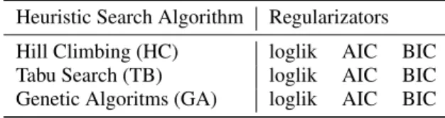
In this work, we compare different heuristics search algorithms along with various regularizations for the likelihood score. In Table 1 we present a list of combinations of the adopted techniques, which are described in details in the subsequent sections. Table 1: Combinations of the different heuristics and regu-larization approaches used in this work.
Heuristic Search Algorithm Regularizators Hill Climbing (HC) loglik AIC BIC Tabu Search (TB) loglik AIC BIC Genetic Algoritms (GA) loglik AIC BIC Here we employ three different and well-known evolutionary methods to solve the previously men-tioned optimization problem, that is to reconstruct the Bayesian network w.r.t. to a specific regularization score. In the rest of this section we briefly describe each method and also the considered regularizators.
3.1 Hill Climbing
Hill Climbing (HC) is one of the simplest iterative techniques that have been proposed for solving
op-timization problems. While HC consists of a simple and intuitive sequence of steps, it is a good search technique to be used as a baseline for comparing the performance of more advanced optimization tech-niques.
Hill climbing shares with other techniques (like simulated annealing (Hwang, 1988) and tabu search (Glover, 1989)) the concept of neighbourhood. Search methods based on this latter concept are itera-tive procedures in which a neighbourhood N(i) is de-fined for each feasible solution i, and the next solution j is searched among the solutions in N(i). Hence, the neighbourhood is a function N : S → 2Sthat assigns
at each solution in the search space S a (non-empty) subset of S. In our case, every solution is modelled as an adjacency matrix, where an entry [i, j] is 1 if in the current solution an arc is present from node i to node
j, and is 0 otherwise.
The sequence of steps of the hill climbing algo-rithm, for a minimization problem w.r.t. a given ob-jective function f , are the following:
1. choose an initial solution i in S;
2. find the best solution j in N(i) (i.e., the solution j such that f ( j) ≤ f (k) for every k in N(i); 3. if f ( j) > f (i), then stop; else set i = j and go to
Step 2.
To counteract the main limitation of hill climbing (i.e., getting trapped in a local optimum), more ad-vanced neighbourhood search methods have been de-fined. The following section presents the Tabu Search method, a popular and effective optimization tech-nique that uses the concept of “memory”.
3.2 Tabu Search
As described in the original work of Glover (Glover, 1989), Tabu Search (TS) is a meta-heuristic that guides a local heuristic search procedure to explore the solution space beyond local optimality. One of the main components of this method is the use of an adap-tive memory, which creates a more flexible search be-haviour. Memory-based strategies are therefore the main feature of TS approaches, founded on a quest for “integrating principles”, by which alternative forms of memory are appropriately combined with effective strategies for exploiting them.
Tabus are one of the distinctive elements of TS when compared to hill climbing or other local search methods. The main idea in considering tabus is to prevent cycling when moving away from local optima through non-improving moves. When this situation occurs, something needs to be done to prevent the search from tracing back its steps to where it came
from. This is achieved by declaring tabu (disallow-ing) moves that reverse the effect of recent moves. For instance, let us consider a problem where solu-tions are binary strings of a prefixed length and the neighbourhood of a solution i consists of the solutions that can be obtained from i by flipping only one of its bits. In this scenario, if a solution j has been obtained from a solution i by changing one bit b, it is possible to declare a tabu to avoid to flip back the same bit b of j for some number of iterations (this number is called the tabu tenure of the move). Tabus are also useful to help the search move away from previously visited portions of the search space and, thus, perform more extensive exploration.
The basic TS algorithm is reported, considering the minimization of the objective function f , as fol-lows:
1. randomly select an initial solution i in the search space S, and set i∗=i and k = 0, where i∗is the
best solution so far and k the iteration counter; 2. set k = k + 1 and generate the subset V of the
ad-missible neighbourhood solutions of i (i.e., non-tabu or allowed by aspiration);
3. choose the best j in V and set i = j; 4. if f (i) < f (i∗), then set i∗=i;
5. update tabu and aspiration conditions;
6. if a stopping condition is met then stop; else go to Step 2.
Commonly used conditions to end the algorithm are when the number of iterations (K) is larger than the maximum number of allowed iterations, or if no changes to the best solution have been performed in the last N iterations (as in our tests).
3.3 Genetic Algorithm
Genetic Algorithms (GAs) are a class of computa-tional models that mimic the process of natural evo-lution (Goldberg and Holland, 1988). GAs are often considered as function optimizers although the range of problems to which genetic algorithms have been applied is quite broad. Although different variants ex-ist, most of the methods called “GAs” have at least the following elements in common: populations of chromosomes, selection according to a fitness func-tion, crossover to produce new offspring, and random mutation of new offspring.
One of the most important issues when using the GAs to solve an optimization problem is the way to encode the candidate solutions, that is the individu-als in the population, and individu-also the genetic operators (crossover and mutation). Since, this aspect strongly
depends on the specific problem, here we describe how GAs have been used to build a Bayesian Net-work. A candidate solution is represented as a string s of length equal to n2, being n the number of nodes
of the network. Each position s[i] can be either 0 or 1, and the information represents the existence of a connection among node i/n and node i%n, where the / operator denotes the integer division, while the % operators denotes the rest of the division between i and n. As an example, s[12] = 1 in a network with 10 nodes means that there is a node between node 1 (12/10) and node 2 (12%10). Nodes are numbered from 0 to n − 1.
To produce admissible solutions (i.e., in our do-main a network without loops), it is fundamental to redefine the classical crossover and mutation opera-tors. More precisely, we developed a simple but effi-cient method that guarantees that crossover and muta-tion will produce Bayesian Networks without loops. To achieve this goal we associated to each solution two lists, called forward list and backward list. The two lists maintain, for each node k, the forward links (i.e., the set of nodes ˆk for which a connection from k to ˆk exists) and the backward links (i.e., the set of nodes ˆk for which a connection from ˆk to k exists). By using these two linked lists it is simple to assess if a new connection between two nodes can be created. In detail, let us assume that the algorithm needs to evalu-ate whether it is possible to add a connection between nodes k1and k2(with k1being the origin and k2the
destination node of the connection). In this scenario, it is necessary to iteratively scan all the elements in the backward list of k1and check if in their backward
lists k2 is present. In this case it would be
impossi-ble to create a connection between k1and k2without
entering a loop in the structure of the network. In the same way, it is necessary to iteratively scan all the el-ements in the forward list of k2and check if in their
forward lists k1is present. Also in this case, the
cre-ation of the connection from k1to k2will introduce a
loop in the network.
Hence, the proposed crossover operator works as follows:
1. choose two individuals p1 and p2 as parents,
based on tournament selection;
2. select a single crossover point for both the parents; 3. for every locus i before that point set child1[i] =
p1[i] and child2[i] = p2[i];
4. for every locus i beyond that point for which p1[i] is equal to p2[i], set child1[i] = p1[i] and
child2[i] = p2[i];
5. for every locus i beyond that point for which p1[i]
• if p2[i] = 0, then set child1[i] = 0 and set
child2[i] = 1 if and only if it is possible to create
a connection between node i/n and node i%n (set child2[i] = 0 in the opposite case);
• if p1[i] = 0, then set child2[i] = 0 and set
child1[i] = 1 if and only if it is possible to create
a connection between node i/n and node i%n (set child1[i] = 0 in the opposite case);
• update the forward and the backward lists. The mutation operator we proposed works as fol-lows:
1. for each locus i of an individual p generate a ran-dom number r from a uniform distribution. If r ≤ pm(where pmis the mutation probability) then
select the locus i for mutation;
2. if p[i] = 1, then set p[i] = 0 and update the forward and backward lists;
3. in the opposite case (p[i] = 0), check if it is pos-sible to create a connection between node i/n and node i%n. If the connection does not introduce a loop set p[i] = 1 and update the data structures, else p[i] will remain equal to 0.
The genetic operators described above ensure that the constraint related to the absence of loops is always satisfied. Moreover, this allows the GA to avoid to reject a high number of individuals that do not respect the constraint. This will result in a beneficial effect on the execution time of the algorithm.
3.4 Regularizators
As already mentioned, we make use of various like-lihood scores as fitness functions for the inference of the network. Such scores, namely loglik, AIC, and BIC, are implemented by using the bnlearn R pack-age (Scutari, 2009).
Specifically, we first considered the log-likelihood score (loglik), that is the logarithm of the previously mentioned likelihood score. Then, as regularized log-likelihood scores, we used the Akaike Information Criterion (AIC) (Akaike, 1992) and the Bayesian In-formation Criterion (BIC) (Schwarz et al., 1978).
To extend this scores in order to model continuous random variables, we adopt the multivariate Gaussian implementation of the log-likelihood score (see (Par-sons, 2011) for a formal definition of the scores and (Scutari, 2009) for the adopted implementation).
4 RESULTS
To assess the performance of the different approaches and regularizators, we have considered the
HPN-DREAM breast cancer network inference challenge. This challenge comprises three sub-challenges, and we focused on the first one (Sub-challenge 1). This sub-challenge consists of two distinct parts: the first one (Sub-challenge 1A) aims at inferring causal sig-nalling networks using protein time-course data. The task spanned 32 different contexts, each defined by a combination of 4 cell lines and 8 stimuli, which fo-cus on networks with specific genetic and epigenetic background. Since for these datasets the real net-work is unknown, beside training data, further data (not used during the inference) are available to assess the causal validity of the inferred networks. The sec-ond part (Sub-challenge 1B) comprises in silico data task and also focused on causal networks. Anyway, differently from the former one, the use of a-priori biology knowledge to design the network is not al-lowed. Since for this sub-challenge the protein net-work is known, the evaluation of the achieved results can be performed by directly comparing the computed network with the original one.
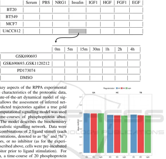
More in details, the datasets of Sub-challenge 1A (“real data”) were generated using Reverse Phase Pro-tein Array (RPPA) quantitative proteomics technol-ogy. RPPA is a protein array designed as a micro- or nano-scaled dot-blot platform that allows the simul-taneous measurement of protein expression levels in a large number of biological samples in a quantita-tive manner, when high-quality antibodies are avail-able (Spurrier et al., 2008). This challenge focuses on about 45 phosphoproteins (proteins phosphory-lated at specific sites). Protein abundance may be in-fluenced by multiple dynamical processes operating over multiple time-scales. This challenge does not focus on long-term changes over days (e.g. rewiring of networks due to epigenetic changes brought about by perturbation), hence data comprises protein time-course data up to 4 hours after ligand stimulation. Time-course data were acquired under 8 ligand stim-uli and inhibition of network nodes by one of 3 in-hibitors plus the vehicle control (cells were serum-starved and pre-treated with inhibitor prior to lig-and stimulation). The experiment was carried out on 4 breast cancer cell lines (namely, BT20, BT549, MCF7, and UACC812), with abundance of the ∼ 45 phosphoproteins measured at 7 time points post-stimulus. Data are normalized protein abundance measurements on a linear scale. Table 2 shows the 32 different processed datasets, obtained by each combi-nation of cell/stimulus, and their compositions, which are the expression levels of the considered phospho-proteins with 4 different inhibitors at 7 consecutive time points.
Table 2: The upper table highlights the 32 combinations of cells/stimuli which constitute the processed “real datasets”. The lower table represents the composition of a single dataset (UACC812/Insulin in the example), which contains the expression levels of the phosphoproteins with 4 inhibitors at 7 different time points.
Serum PBS NRG1 Insulin IGF1 HGF FGF1 EGF BT20 BT549 MCF7 UACC812 0m 5m 15m 30m 1h 2h 4h GSK690693 GSK690693 GSK1120212 PD173074 DMSO
to mimic the key aspects of the RPPA experimental set up and the characteristics of the proteomic data, but using a state-of-the-art dynamical model of sig-nalling. This allows the assessment of inferred net-works and predicted trajectories against a true gold standard. A computational signalling model was used to generate time-courses of phosphoprotein abun-dance levels. The model describes the biochemistry underlying a realistic signalling network. Data were generated for combinations of 2 ligand stimuli (each one at 2 concentrations, denoted to as “lo” and “hi”) and 3 inhibitors, or no inhibitor (as for the experi-mental data described above, cells were pre-incubated with the inhibitor prior to ligand stimulation). For each condition, a time-course of 20 phosphoprotein levels is provided at 10 time points post-stimulus. It must be noticed that phosphoprotein names have been anonymized so that detailed prior information from canonical signalling pathways cannot be used. Efforts have been made to model the antibody-based readout of the RPPA platform and its technical variability in a faithful manner. Three technical replicates are pro-vided per condition. Data propro-vided to participants are protein abundance measurements on a linear scale. In this task, a single network should be inferred in con-trast to the proteomic data challenge that requires 32 networks.
Following the approach used to evaluate the re-sults submitted to the challenge, we have considered the same method to assess the performance of our predictions. More precisely, in real data, for any given context, the set of nodes that showed salient changes under a test inhibitor (here an mTOR in-hibitor) relative to the control was identified. These
Figure 1: Mean results on the 32 experimental datasets for the considered approaches.
“gold-standard” sets are derived from (held-out) ex-perimental data and should not be regarded as resenting a fully definitive ground truth. For each dicted network, the set of mTOR descendants is pre-dicted and compared against the experimental one to obtain the area under the receiver operating charac-teristic curve (AUROC) score (Hill et al., 2016). Re-sults are ranked in each of the 32 contexts by AUROC score, and the mean rank across contexts was used to provide an overall score and a final ranking. For the in silico data task, the true causal network was known and it was used to obtain an AUROC score for each predicted network. This score has been considered to determine the final ranking.
By analysing the mean AUROC values computed on the predictions on the 32 real datasets, which are
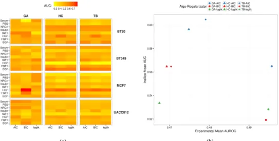
(a) (b)
Figure 2: (a)Heatmap showing the AUC values obtained with each combination of heuristic search method and regulariza-tor on the 32 experimental datasets. (b) Scores in experimental and in silico data tasks. Each combination of shape/color corresponds to a specific algorithm/regularizator pair.
reported as bars in the plots in Figure 1, it is possible to observe that all the tested approaches have similar performance, with mean values around 0.5.
Anyway, when looking more in details on each of the 32 datasets, we can draw more accurate con-siderations about the behaviour of the tested tech-niques. In particular, as showed in the heatmap in Figure 2(a), on the processed datasets we have ob-tained AUROC values ranging from 0.3 to 0.7. As corroborated by several studies present in literature, these results highlight the fact that HC (hill climbing) and TB (tabu search) have almost the same behaviour, also, w.r.t. the considered regularizator, on the major-ity of the datasets. On the other hand, GA (genetic al-gorithm) presents slightly different results than those obtained by the other two methods and, moreover, it seems that the results are affected by the considered regularizator. Interestingly, when looking at the in sil-ico AUC values, we can observe that, for each reg-ularizator, HC and TB perform better on the in sil-ico dataset, while GA is slightly worse; the opposite situation is observed in the real datasets, where the latter method (i.e. genetic algorithms) achieves bet-ter results with respect to the two former techniques (i.e., hill climbing and tabu search). The scatter plot in Figure 2(b) shows a comparison of the mean AUC results on the in silico dataset against the AUROC mean values on the real datasets obtained with all the employed approaches.
To assess the quality of the obtained results, we performed a comparison with those obtained by the participants of the challenge. More precisely, as re-ported in (Hill et al., 2016), several different tech-niques have been used to reconstruct the network
pro-posed in this challenge, which can be distinguished based on the fact that a prior knowledge has been em-ployed in order to improve the predictions, and also based on the reconstruction method (Bayesian net-works in our case). From the results on the in sil-ico dataset, ranked by the mean AUC, we observed that our best performer (TB with AIC) obtained a value of 0.6, which is better than all the other meth-ods based on Bayesian networks and ranks in the top 15% of the overall evaluated techniques. On the other hand, on the 32 real datasets our results are similar to those obtained by methods based on Bayesian net-works, which present values around 0.5. Both these results are not surprising, since we do not use any prior knowledge on the input data (resulting in good performance on the in silico dataset), and also the number of observations in each of the 32 real datasets is quite low compared to the number of nodes (phos-phoprotein) of the networks to reconstruct, hence pe-nalizing Bayesian approaches, making the inference task difficult.
5 CONCLUSIONS
In this work, we studied the inference of causal molecular networks, specifically focusing on signal-ing downstream of receptor tyrosine kinases. We modeled relationships (edges) in causal molecular networks (’causal edges’) as directed links between nodes, in which inhibition of the parent node can lead to a change in the abundance of the child node, either by direct interaction or via unmeasured intermediate nodes.
To this extent, we have tested different methods to reconstruct (Bayesian) networks on real and in sil-ico datasets proposed in the HPN-DREAM challenge. Specifically, we analyzed the performance of different optimization search schemes, i.e., Hill climbing (HC), Tabu seach (TS) and Genetic algorithms (GA), and various likelihood scores, i.e., loglik, AIC and BIC. This analysis seems to show a better performance of more sophisticated search strategies like GA on real datasets, even if on in silico data it is shown that eas-ier search schemes as HC and TS also prove to be very effective.
Furthermore, we find the obtained results to be en-couraging, especially considering the fact the we have employed “standard” versions of the algorithms for the reconstruction of the network without making use of any biological prior.
REFERENCES
Akaike, H. (1992). Information theory and an extension of the maximum likelihood principle. In Breakthroughs in statistics, pages 610–624. Springer.
Akutsu, T., Miyano, S., Kuhara, S., et al. (1999). Identi-fication of genetic networks from a small number of gene expression patterns under the boolean network model. In Pacific symposium on biocomputing, vol-ume 4, pages 17–28. Citeseer.
Bansal, M., Belcastro, V., Ambesi-Impiombato, A., and Di Bernardo, D. (2007). How to infer gene networks from expression profiles. Molecular systems biology, 3(1):78.
Friedman, N., Linial, M., Nachman, I., and Pe’er, D. (2000). Using bayesian networks to analyze expression data. Journal of computational biology, 7(3-4):601–620. Glover, F. (1989). Tabu search-part i. ORSA Journal on
computing, 1(3):190–206.
Goldberg, D. E. and Holland, J. H. (1988). Genetic al-gorithms and machine learning. Machine learning, 3(2):95–99.
Hill, S. M., Heiser, L. M., Cokelaer, T., Unger, M., Nesser, N. K., Carlin, D. E., Zhang, Y., Sokolov, A., Paull, E. O., Wong, C. K., et al. (2016). Inferring causal molecular networks: empirical assessment through a community-based effort. Nature methods, 13(4):310– 318.
Hwang, C.-R. (1988). Simulated annealing: theory and applications. Acta Applicandae Mathematicae, 12(1):108–111.
Imoto, S., Goto, T., Miyano, S., et al. (2001). Estimation of genetic networks and functional structures between genes by using bayesian networks and nonparametric regression. In Pacific symposium on Biocomputing, volume 7, pages 175–186.
Kabir, M., Noman, N., and Iba, H. (2010). Reverse engi-neering gene regulatory network from microarray data using linear time-variant model. BMC bioinformatics, 11(1):1.
Parsons, S. (2011). Probabilistic graphical models: Prin-ciples and techniques. The Knowledge Engineering Review, 26(02):237–238.
Pearl, J. (2003). Causality: models, reasoning and infer-ence. Econometric Theory, 19:675–685.
Schramm, G., Kannabiran, N., and K¨onig, R. (2010). Reg-ulation patterns in signaling networks of cancer. BMC systems biology, 4(1):1.
Schwarz, G. et al. (1978). Estimating the dimension of a model. The annals of statistics, 6(2):461–464. Scutari, M. (2009). Learning bayesian networks with the
bnlearn r package. arXiv preprint arXiv:0908.3817. Spurrier, B., Ramalingam, S., and Nishizuka, S. (2008).
Reverse-phase protein lysate microarrays for cell sig-naling analysis. Nature protocols, 3(11):1796–1808. Stolovitzky, G., Monroe, D., and Califano, A. (2007).
Di-alogue on reverse-engineering assessment and meth-ods. Annals of the New York Academy of Sciences, 1115(1):1–22.
Zou, M. and Conzen, S. D. (2005). A new dynamic bayesian network (dbn) approach for identifying gene regulatory networks from time course microarray data. Bioinformatics, 21(1):71–79.