Digital mapping of soil attributes using machine learning
1Mapeamento digital de atributos do solo utilizando aprendizado de máquina
Patrícia Morais da Matta Campbell2*, Márcio Rocha Francelino3, Elpídio Inácio Fernandes Filho3, Pablo de Azevedo Rocha3 and Bruno Campbell de Azevedo4
ABSTRACT - Mapping the chemical attributes of the soil on a large scale can result in gains when planning the use and occupation of the land. There are different techniques available for this purpose, whose performance should be tested for different types of landscapes. The aim of this study was to spatialize chemical attributes of the soil, comparing eight methods of prediction. Forty morphometric attributes, generated from a digital elevation model, were used as independent variables, in addition to geophysical data, images from the Landsat 8 satellite and the NDVI. All possible combinations between the satellite bands were calculated, generating 28 new variables. Combinations between the Th, U and K bands obtained from the geophysical data were also calculated, generating a further three variables. The final variables to be calculated were the distances between the four points of the edges of the basin (d1, d2, d3 and d4). The dependent variables for the model were Al, Ca, Fe, K, Mg, Na, Si, Ti, Cr, Cu, Mn, Ni, P, Pb, V, Zn, Zr, S and Cl. A total of 200 soil samples were used, which were collected from 100 points at two depths (0-10 and 10-30 cm); the total elements were determined using an X-ray fluorescence analyzer. The Random Forest algorithm proved to be superior to the others in predicting the chemical attributes of the soil at both depths, and is suitable for predicting soil attributes in the study region. Spatial variables are essential, and should be considered when modelling chemical elements in the soil. Using the methods under test, it is possible to predict elements with R² values ranging from 0.32 to 0.62.
Key words: XRF. Spatial approach. Prediction models.
RESUMO - O mapeamento de atributos químicos do solo em larga escala pode acarretar em ganhos no planejamento de uso e ocupação do mesmo. Existem diferentes técnicas disponíveis para tal fim, cujos desempenhos devem ser testados para diferentes situações de paisagem. Objetivou-se neste trabalho espacializar atributos químicos do solo, comparando oito métodos para predição. Como variáveis independentes foram utilizados 40 atributos morfométricos gerados a partir do modelo digital de elevação, além de dados geofísicos, imagens do satélite Landsat 8 e o NDVI. Calculou-se todas combinações possíveis entre as bandas do satélite, gerando 28 novas variáveis. Também foram feitas combinações entre as bandas de Th, U e K obtidas dos dados geofísicos, gerando outras três variáveis. As últimas variáveis calculadas foram as distâncias entre os quatro pontos das extremidades da bacia (d1, d2, d3 e d4). As variáveis dependentes do modelo foram teores de Al, Ca, Fe, K, Mg, Na, Si, Ti, Cr, Cu, Mn, Ni, P, Pb, V, Zn, Zr, S e Cl. Foram utilizadas 200 amostras de solo, coletadas em 100 pontos em duas profundidades (0-10 e (0-10-30 cm), e os elementos totais foram determinados em analisador de fluorescência de raios-X. Random Forest mostrou-se superior aos demais para predizer os atributos químicos do solo nas duas profundidades, mostrou-sendo indicado para predição dos atributos dos solos da região de estudo. As variavéis espaciais mostraram-se altamente prescindíveis, devendo ser consideradas nas modelagens dos elementos químicos do solo. É possível a predição dos elementos com R² variando de 0,32 a 0,62 pelos métodos testados.
Palavras-chave: XRF. Abordagem espacial. Modelos de predição. DOI: 10.5935/1806-6690.20190061
*Author for correspondence
Received for publication 26/04/2018; approved on 05/03/2019
1Trabalho extraído da Tese do primeiro autor apresentada ao Programa de Pós-graduação em Ciências Ambientais e Florestais, Universidade
Federal Rural do Rio de Janeiro/UFRRJ
2Programa de Pós-Graduação em Ciências Ambientais e Florestais, Departamento de Silvicultura e Manejo Florestal, Universidade Federal Rural do
Rio de Janeiro, Seropédica-RJ, Brasil, [email protected] (ORCID ID 0000-0001-8507-8496)
3Departamento de Solos, Universidade Federal de Viçosa, Viçosa-MG, Brasil, [email protected] (ORCID ID 0000-0001-8837-1372),
[email protected] (ORCID ID 0000-0002-9484-1411), [email protected] (ORCID ID 0000-0001-9581-9622)
4Programa de Pós-Graduação em Agricultura Orgânica, Departamento de Fitotecnia; Universidade Federal Rural do Rio de Janeiro, Seropédica-RJ,
INTRODUCTION
New computational techniques have been presented as an alternative tool for mapping soil classes and attributes, providing greater speed, repeatability and error recognition, which are seen as the greatest advantages over conventional methods (PINHEIRO et al., 2012). Due to the increasing need for more-detailed information on soils for various applications, digital methods can contribute significantly when planning land use and occupation.
Digital mapping is based on the SCORPAN model, in which a given soil class is a function of five factors of the ClORPT model (climate - Cl, organisms - O, relief - R, parent material - P and time - T), added to the factors of soil (s), and spatial or geographic position (n) (McBRATNEY
et al., 2003). This new model not only allows the classes
of soil to be mapped, but also the soil attributes.
Since the end of the 1960s, there has been an emphasis on what might be termed “geographical” or “purely spatial” approaches, i.e. soil attributes would be predicted from spatial position, largely by interpolation between the observation sites (McBRATNEY et al., 2003).
As such, some studies began to test the use of spatiality to predict the attributes, not only of soils, but also other elements of the physical environment (DAVIES; GAMM, 1969; KISS et al., 1988), with the appearance of such interpolation methods as kriging, among others. However, the use of spatial tools alone has led to the development of models where the trend surfaces are fairly simplified and “artificial” representations, and where the more complex spatial patterns generally need to be modeled (McBRATNEY
et al., 2003).
This led to the adoption of hybrid models that combine different methods, such as the use of classifying algorithms like Random Forest and kriging. These are combined with the aim of improving both techniques, always including the spatial component, which is a potentially valuable and economical source of environmental information, and should never be disregarded (ARRUDA; DEMATTE; CHAGAS, 2013; McBRATNEY et al., 2003).
Various factors derived from the digital elevation model (DEM) have been tested as predictor variables (MENEZES et al., 2014; OLIVEIRA et al., 2012; PINHEIRO et al., 2012; RYAN et al., 2000; YANG et al., 2016) in different methods for generating digital maps. Several techniques have been evaluated for mapping attributes, among them neural networks, decision trees and multiple linear regression. However, no studies were found in the literature that mapped a high number of chemical
elements in the soil, using, in addition to environmental covariates, spatial variables as predictors.
Under the hypothesis that there may be algorithms which are more efficient in predicting a large number of soil attributes with good R² values, where spatial variables may prove to be essential to the model, this work aimed to map the chemical attributes of the soil (the levels of Al, Ca, Fe, K, Mg, Na, Si, Ti, Cr, Cu, Mn, Ni, P, Pb, V, Zn, Zr, S, Cl) in a drainage basin located in the district of Iconha, Espírito Santo (ES), at two depths, using environmental and spatial covariates as predictors and comparing predictions of the Random Forest, Ridge Regression, Cubist and Partial Least Squares methods; principal component regression (PCR); Adaptive Forward-Backward Greedy Algorithm (FOBA); Generalized Boosted Regression Models (GBM) and Gradient Boosting with Component-wise Linear Models (GLMBOOST).
MATERIAL AND METHODS
The work was carried out in the drainage basin of the Ribeirão Inhaúma; an area of 2,403.9 ha, centered on 21°10’58.82” S and 41°00’08.87” W, and located in the district of Iconha, in the south of the state of Espírito Santo. In order to predict the chemical attributes of the soil, it was necessary to determine the independent variables that would be tested. The digital elevation model (DEM), obtained with data from the ALOS Satellite (Advanced Land Observing Satellite) at a spatial resolution of 12.5 m, was used to generate 37 morphometric covariates (Table 1), using a script developed in the R software (RSaga) for applying the terrain-analysis tools included in the free SAGA software (BÖHNER; MCCLOY; STROBL, 2006) together with the land use and occupation map.
The Landsat 8 (LS8) satellite bands were also used as independent variables, the NDVI (Normalized Difference Vegetation Index) was calculated using the LS8 bands in the equation proposed by Rouse et al. (1973), where it is expressed as the ratio between the difference
in reflectance measured in the near red (ρ-IV) and infrared
(ρ-V) channels, and the sum of these channels, so:
(1) Aerogeophysical data, such as gamma spectrometry and magnetometry, obtained from the Mineral Resources Research Company (Companhia de Pesquisa de Recursos
Minerais - CPRM), were also used (Table 1).
All possible combinations between the bands were calculated, generating 28 new spectral covariates. These were obtained, by means of the relation:
(2)
where: Bxy is the result of the band x to band y ratio,
and bx and by represent the Landsat 8 satellite bands.
For the variables derived from the gamma spectrometry, the same ratio was used as in equation 2, where combinations were made between the estimated
values of thorium (Th), uranium (U) and potassium (K),
generating three new variables. The distances between the four points at the edges of the basin (d1, d2, d3 and d4) were calculated as per the relation:
(3)
Table 1 - Independent variables used to predict chemical attributes of the soil
Derivatives of the digital elevation model
Convergence index Mid-Slope Position Total Curvature
Cross-Sectional Curvature Minimal Curvature Total Insolation1
Curvature Classification Digital Elevation Model Total Insolation2
Diffuse Insolation1 Normalized Height Valley Depth
Diffuse Insolation2 Plan Curvature Valley Index
Direct to Diffuse Ratio1 Profile Curvature
Direct to Diffuse Ratio2 Real Surface Area
Diurnal Anisotropic Slope
Duration of Insolation1 Slope Height
Duration of Insolation2 Slope Index
Flow-Line Curvature Standardized Height
General Curvature Surface-Specific Points
Landforms Tangential Curvature
Longitudinal Curvature Terrain Surface Texture
Mass Balance Terrain Surface Convexity
Maximal Curvature Topographic Wetness Index
Geophysical data Others
Total Magnetic Field Landsat8 Bands
Total Count NDVI
Potassium Use and occupation map
First Derivative of the Total Magnetic Field Band Ratio
Thorium to Potassium Ratio Th to U to K Ratio
Uranium to Potassium Ratio Distances between points
Uranium to Thorium Ratio x,y Coordinates
Analytic Signal of the Total Magnetic Field Total Exposure Count Rate
Thorium Uranium
where: dAB is the distance between two points A and B, x2
and y2 are the coordinates of point A and x1 and y1 are the
coordinates of point B.
The x and y coordinates were also considered as variables, i.e. latitude and longitude. All the maps were standardized with the same size of cells, lines and columns, and a resolution of 30 m. The maps from the MDE were re-sampled using the ArcGis 10.1 software.
The levels of Al, Ca, Fe Al, Ca, Fe, K, Mg, Na, Si, Ti, Cr, Cu, Mn, Ni, P, Pb, V, Zn, Zr and S were used as the dependent variables for the model. In order to obtain values for the attributes, 200 soil samples were collected in the field at a depth of 0-10 cm and 10-30 cm. The conditioned
Latin hypercube method was used to set up the sampling grid, due to difficulty in accessing the area caused by the extremely mountainous relief. The coordinates of each sampling point were recorded with the Leica GS08 Plus GNSS receiver. The data were processed using the Leica Geoffice 8.0 software, employing the fixed station of the Brazilian Institute of Geography and Statistics (IBGE) in Vitória, ES, for transportation from the base to the area of the basin.
The soil samples were air dried, the clumps were removed, and the soil sieved through a 2-mm aperture mesh. In the laboratory, the samples were macerated in an agate mortar, sieved through a 1-mm aperture mesh, and then placed in a standard mold and manually compressed to form tablets, 15 mm in diameter and 2 mm thick, that were used to take readings in the X-ray fluorescence analyzer of the Soil Laboratory (ALVES et al., 2015) of the Federal University of Viçosa - UFV, to obtain the total content of the elements in each sample. For this, the Shimadzu Micro-EDX-1300 analyzer was used.
Results that presented outliers were identified and their data replaced with values estimated by means of regression imputation, where the new value is calculated through regression of the other values of the variable, thereby avoiding a reduction in the number of analytical data.
The response variables at both sampling depths were tested for normality by means of the Kolmogorov-Sminorv test (K-S) (p<0.05).
Attribute maps were generated using the R v3 software. To select the most important independent variables, those with a correlation index greater than 0.99 were eliminated. Subsequently, each model selected the most significant variables to predict each of the attributes, these being used to generate the final maps. Simplified models were sought, i.e. models that used the smallest possible number of variables with satisfactory R² values, where a loss of up to 5% in the R² values was allowed in favor of a more economical model.
Point values for each of the independent variables were extracted using the ArcGis software, employing the ‘extract value to points’ command. In order to have greater area representativity, the mean of the central point with its neighbors was considered as a typical value for the sampled site.
The performance of the models was evaluated using the cross-validation procedure with 10 repetitions, in which comparisons were made between the observed and predicted values of each dependent variable. These values were expressed by the coefficient of determination R². The index was calculated according to the equation:
(4) where: Pi e Oi are the predicted and observed values at location i respectively, and n is the number of samples.
The RMSE value (root mean square error) was also calculated.
(5) where: RMSE is the root mean square error, and Ɩ is the number of points intended for validation.
RESULTS AND DISCUSSION
In relation to the predictions of the models under test, only those elements whose R² value was greater than 0.30 for at least one of the methods are presented. As a result, the applied methods were not efficient in predicting Ca, Mg, Na, Si, Cr, Cu, Ni and Zr at the depth of 0-10 cm, or Mg, Na, Si, Cu, Mn, Ni and Zn at 10-30 cm.
Table 2 shows the descriptive statistics for the modelled elements at both depths, i.e. Al, Fe, K, Mn, P, Pb, S, Ti, V and Zn at 0-10 cm, and Al, Ca, Cr, Fe, K , P, Pb, S, Ti, V and Zr at 10-30 cm.
With the set of data from the first depth, a negative asymmetric distribution was seen for Al, K and Zn, and a positive asymmetric distribution for the remainder, while at a depth of 10-30 cm, negative asymmetric distribution occurred only for Al and Fe. With positive asymmetry, mean values are generally higher than the median, indicating a high frequency of values below the mean (LIMA et al., 2010). Such behavior was seen for P, S and Zn at 0-10 cm and for all the elements at 10-30 cm, except Fe.
Negative asymmetry indicates concentration of the data (tail elongation) to the left of the mean, and positive asymmetry shows the data concentrated to the right of the mean. Values closer to zero indicate greater symmetry and, therefore, normal data distribution (GROENEVELD; MEEDEN, 1984).
Kurtosis indicates the degree of data flattening, where the distribution is classified as leptokurtic (when the kurtosis value is <0.263), mesocurtic (=0.263) or platicurtic (>0.263). At both depths, the data have a leptokurtic distribution, characterized by a more funneled curve, with a higher peak than normal (mesocurtic), except for P and S (0-10 cm) and Ca (10-30 cm), which have a platicurtic distribution, this curve being flatter than either the mesocurtic or leptokurtic.
Table 2 - Descriptive analysis of the chemical attributes of the soil at a depth of 0-10 cm and 10-30 cm
*Al, Ca, Fe, K, S, Ti in dag/kg, and Cr, Mn, P, Pb, V, Zn, Zr in ppm
Depth 0-10 cm
Variable* Mean Median Standard Deviation Minimum Maximum Asymmetry Kurtosis
Al 24.88 24.94 4.44 13.76 35.45 -0.33 -0.02 Fe 10.37 10.65 2.76 3.51 17.73 0.003 -0.15 K 1.22 1.25 0.48 0.14 2.22 -0.26 -0.54 Mn 601.40 600.68 315.16 53.50 1314.77 0.24 -0.69 P 2359.64 2082.35 1394.97 0.00 5867.08 0.46 -0.52 Pb 198.65 200.39 69.78 57.27 395.50 0.20 -0.24 S 0.12 0.11 0.05 0.03 0.30 1.02 1.13 Ti 2.12 2.13 0.67 0.97 3.45 0.14 -1.06 V 417.78 424.47 133.77 210.05 719.71 0.15 -1.08 Zn 119.01 118.53 42.78 28.68 232.19 -0.02 -0.41 Depth 10-30 cm Al 25.02 24.75 4.93 13.44 33.86 -0.15 -0.67 Ca 0.20 0.19 0.13 0.01 0.61 0.93 1.17 Cr 289.28 272.04 109.92 18.12 541.42 0.23 -0.32 Fe 10.36 10.43 2.80 3.31 17.56 -0.13 0.09 K 1.27 1.27 0.31 0.10 2.57 0.15 -0.20 P 2133.07 1736.18 1340.61 0.00 5981.57 0.79 0.18 Pb 202.47 199.63 78.71 61.00 429.81 0.52 0.03 S 0.11 0.10 0.02 0.01 0.22 0.49 -0.37 Ti 2.16 2.14 0.70 0.93 3.80 0.20 -0.83 V 427.82 423.37 139.62 183.15 745.18 0.20 -0.95 Zr 727.76 709.67 223.03 249.38 1315.95 0.50 -0.05
For the predictive variables, those showing a correlation equal to or greater than 0.99 were eliminated. These were: Diffuse Insolation2, Total Insolation2, Valley Index, and Landsat 8 Bands 2 and 4.
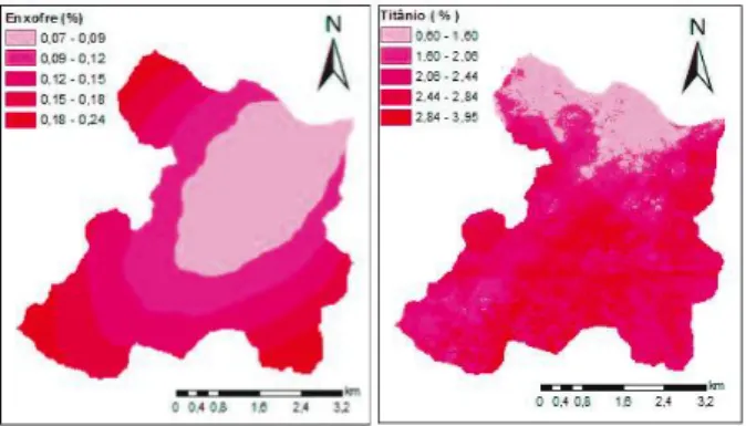
At the depth of 0-10 cm, the R² values (Table 3), calculated based on the regression between the observed values and those predicted by the models, show that RF was superior for three of the variables (Fe, Mn and V), with RIDGE superior for two (S and Zn) and the remainder (PLS) for one. PLS and PCR were equally efficient for predicting P (R² = 0.42), while RIDGE, cubist, PLS, PCR and FOBA for Ti (R² = 0.50). R² values at this layer ranged from 0.23 to 0.54.
Regarding the lowest R² values, FOBA stood out for not presenting any of the lower correlation coefficients. For Al, Mn, P and Pb, more than one method presented the lower values. In general, PLS, PCR, GBM and GLMBOOST presented lower predicted R² values.
In relation to the elements, the highest R2 values
were found for Ti (0.50) and V (0.54). Ti minerals are very weather resistant; apparently under reducing conditions
Fe2+ ions are adsorbed on the surfaces of Ti minerals,
Ti being able enter the structure of some silicates and probably adsorbed on the surface of Fe-Mn concretions. As it is one of the most stable elements, Ti is present in small amounts in the soil solution, about 0.03 mg/L, (KABATA-PENDIAS, 2010).
V is distributed fairly uniformly in soil profiles, and variations in soil content are inherited from the parent materials (KABATA-PENDIAS, 2010). As such, the highest concentrations of V (up to 500 mg/kg) are reported for Cambisols (KABATA-PENDIAS, 2010), levels which probably facilitate their mapping, since this type of soil is widely distributed over the study area. The V in soils seems to be mainly associated with hydrated Fe oxides and with organic matter. In some soils, clay minerals
can also control the mobility of this element (KABATA-PENDIAS, 2010).
As expected, the RMSE values (Table 4) tended to be smaller the higher the R² value. In predicting P, where R² was the same for both PLS and PCR, it can be inferred that PCR was superior due to the lower RMSE value. However, the same was not possible for S or Ti, whose RMSE values remained the same for the best predictors.
In the 10-30 cm layer, there was greater disparity as to the best predictor in relation to the R² values (Table 5). In general, soil attributes vary continuously with depth in the soil profile (RUSSELL; MOORE, 1968), which
Element Method
RF RIDGE CUBIST PLS PCR FOBA GBM GLMBOOST
Al 0.39 0.37 0.35 0.33 0.33 0.38 0.33 0.40 Fe 0.49 0.41 0.44 0.40 0.41 0.43 0.45 0.41 K 0.40 0.34 0.36 0.34 0.23 0.35 0.41 0.33 Mn 0.38 0.31 0.32 0.31 0.32 0.33 0.36 0.31 P 0.37 0.39 0.39 0.42 0.42 0.40 0.37 0.40 Pb 0.39 0.36 0.42 0.37 0.37 0.38 0.40 0.36 S 0.36 0.38 0.33 0.37 0.37 0.38 0.35 0.37 Ti 0.48 0.50 0.50 0.50 0.50 0.50 0.46 0.48 V 0.54 0.48 0.52 0.50 0.50 0.48 0.52 0.45 Zn 0.37 0.39 0.30 0.27 0.24 0.37 0.36 0.38 Element* Method
RF RIDGE CUBIST PLS PCR FOBA GBM GLMBOOST
Al 3.79 3.99 3.96 3.88 3.87 3.82 3.92 3.77 Fe 2.04 2.21 2.18 2.21 2.21 2.16 2.13 2.18 K 0.38 0.42 0.40 0.42 0.44 0.40 0.38 0.41 Mn 257.28 272.11 269.69 270.89 269.45 266.48 260.67 270.95 P 1098.40 1058.68 1082.61 1037.59 1035.29 1053.91 1079.42 1054.49 Pb 62.42 62.78 61.76 62.24 62.23 61.54 62.01 62.23 S 0.04 0.04 0.04 0.04 0.04 0.04 0.04 0.04 Ti 0.50 0.48 0.48 0.48 0.48 0.48 0.51 0.50 V 92.17 98.36 95.23 96.66 96.65 98.24 95.13 102.51 Zn 35.06 35.58 37.69 38.99 39.18 36.08 35.68 35.06
Random Forest-RF, Ridge Regression-RIDGE, Partial Least Squares-PLS, Principal Component Regression-PCR, Adaptive Forward-Backward Greedy Algorithm-FOBA, Generalized Boosted Regression Models-GBM and Gradient Boosting with Component-wise Linear Models – GLMBOOST Table 3 - R2 values generated by the three methods for predicting chemical attributes of the soil at a depth of 0-10 cm
can generate differences in the prediction ability of each model. RF was highlighted in six variables (Al, Ca, Fe, K, P and Pb) and was equal to FOBA for the variable Zr, with R² = 0.34. FOBA was superior for Cr, GBM for Ti and V, and PLS and PCR obtained the same R² value for S (0.37).
The R2 values ranged from 0.24 to 0.62.
As in the 0-10 cm layer, V and Ti were the elements with the best prediction, presenting an R² of 0.62 and 0.56 respectively. RIDGE, cubist and GLMBOOST proved not to be efficient predictors in the 0-30 cm layer, obtaining none of the higher R² values, and having some of the lowest values found for the correlation coefficient. FOBA,
Table 4 - RMSE values found for Al, Fe, Mn, P, Pb, S, Ti, V and Zn in the 0-10 cm layer, for the different methods under test
*Al, Fe, K, S, Ti in dag/kg, and Mn, P, Pb, V Zn in ppm. Random Forest-RF, Ridge Regression-RIDGE, Partial Least Squares-PLS, Principal Component Regression-PCR, Adaptive Forward-Backward Greedy Algorithm-FOBA, Generalized Boosted Regression Models- GBM and Gradient Boosting with Component-wise Linear Models – GLMBOOST
just as in the 0-10 cm layer, obtained none of the lower R² values, the same as RF in this layer.
RMSE behavior in the 10-30 cm layer was similar
to the first layer, i.e. the lowest values were generally
found for the highest estimates of R² (Table 6). The only exception was for P, where the lowest RMSE value was obtained with RIDGE. With lower RMSE values, it can be inferred that RF was superior to FOBA in predicting Zr, whose R² had been similar. S presented its highest R² values with the PLS and PCR methods, however with similar RMSE values in all methods.
Among the predictors under test, RF is the most common in studies found in the literature, being employed to predict various soil properties (CAMERA et al., 2017). These properties, however, are generally related to texture (sand, silt, clay) (BISHOP et al., 1999; CHAGAS et al., 2016; HEUVELINK et al., 2016; LAGACHERIE et al., 2008; MA
et al., 2017; VAYSSE; LAGACHERIE, 2015); chemical,
focusing on pH (BISHOP et al., 1999; DHARUMARAJAN
et al., 2017; HEUVELINK et al., 2016; MA et al., 2017;
MALONE et al., 2014; VÅGEN et al., 2016; VAYSSE; LAGACHERIE, 2015); organic carbon (ADHIKARI
Table 5 - R2 values generated by the three methods for predicting chemical attributes of the soil at a depth of 10-30 cm
Random Forest-RF, Ridge Regression-RIDGE, Partial Least Squares-PLS, Principal Component Regression-PCR, Adaptive Forward-Backward Greedy Algorithm-FOBA, Generalized Boosted Regression Models- GBM e Gradient Boosting with Component-wise Linear Models – GLMBOOST
Table 6 - RMSE values found for Al, Ca, Cr, Fe, K, P, Pb, S, Ti, V and Zr in the 10-30 cm layer, for the different methods under test
*Al, Ca, Fe, K, S, Ti in dag/kg, and Cr, P, Pb, V, Zr in ppm. Random Forest-RF, Ridge Regression-RIDGE, Partial Least Squares-PLS, Principal Component Regression -PCR, Adaptive Forward-Backward Greedy Algorithm-FOBA, Generalized Boosted Regression Models- GBM e Gradient Boosting with Component-wise Linear Models – GLMBOOST
Element Method
RF RIDGE CUBIST PLS PCR FOBA GBM GLMBOOST
Al 0.37 0.28 0.31 0.29 0.30 0.32 0.36 0.33 Ca 0.32 0.29 0.26 0.24 0.24 0.31 0.28 0.29 Cr 0.26 0.32 0.24 0.33 0.32 0.35 0.28 0.32 Fe 0.43 0.33 0.35 0.33 0.33 0.34 0.39 0.33 K 0.38 0.35 0.32 0.36 0.36 0.36 0.36 0.36 P 0.45 0.36 0.37 0.42 0.43 0.40 0.40 0.39 Pb 0.32 0.21 0.25 0.29 0.30 0.25 0.30 0.23 S 0.32 0.32 0.32 0.37 0.37 0.32 0.30 0.30 Ti 0.52 0.42 0.44 0.44 0.44 0.44 0.56 0.43 V 0.55 0.52 0.52 0.50 0.50 0.55 0.62 0.52 Zr 0.34 0.28 0.27 0.28 0.28 0.34 0.28 0.31 Element* Method
RF RIDGE CUBIST PLS PCR FOBA GBM GLMBOOST
Al 4.10 4.61 4.38 4.50 4.47 4.34 4.15 4.25 Ca 0.23 0.24 0.24 0.24 0.24 0.23 0.23 0.23 Cr 100.42 94.74 102.97 94.90 94.99 92.03 97.81 94.32 Fe 2.35 2.55 2.52 2.54 2.54 2.52 2.46 2.55 K 0.45 0.47 0.47 0.46 0.46 0.46 0.45 0.46 P 1063.33 943.15 1031.79 972.34 966.61 991.67 991.74 1005.35 Pb 71.13 82.70 76.68 73.21 72.99 76.79 72.37 76.53 S 0.04 0.04 0.04 0.04 0.04 0.04 0.04 0.04 Ti 0.50 0.55 0.54 0.54 0.54 0.54 0.48 0.54 V 95.76 100.57 99.59 101.79 101.79 97.11 89.07 99.27 Zr 215.96 234.96 235.68 229.85 229.46 219.65 229.07 226.21
et al., 2014; AKPA et al., 2016; BISHOP et al., 1999;
DHARUMARAJAN et al., 2017; GOMEZ et al., 2008; GRIMM et al., 2008; GUO et al., 2015; HEUVELINK
et al., 2016; MA et al., 2017; POGGIO et al., 2013;
RAMIFEHIARIVO et al., 2017; SREENIVAS et al., 2016; VÅGEN et al., 2016; WIESMEIER et al., 2011); electrical conductivity (BISHOP et al.,1999; DHARUMARAJAN
et al., 2017; VAYSSE; LAGACHERIE, 2015), and cation
exchange capacity (CHAGAS et al., 2016; LAGACHERIE
et al., 2008; VÅGEN et al., 2016).
Hengl et al. (2015) found negative R2 values when
mapping exchangeable sodium using linear regression. The authors found a gain in R² when comparing the mapping of exchangeable bases, especially Ca and Mg, made with RF in relation to the regression. No predictions carried out by the methods tested in this study were found in the literature in relation to elements obtained by x-ray fluorescence.
For the principal variables used in the prediction models, in the 0-10 cm layer half of the mapped elements (Al, Fe, K, Pb and S) considered the geophysical data to be important variables. The following should be mentioned: the ratio of uranium to potassium (Al, Pb), the ratio of thorium to potassium (Al, S), uranium (pb), potassium (Al, S), thorium (K) and the analytic signal of the total magnetic field (Al, Fe, Pb).
For the 10-30 cm layer, with the exception of Fe, all the elements considered the geophysical data to be important. Including the ratio of uranium to potassium (Al, Ca), the ratio of thorium to potassium (Ca, S), the ratio of uranium to thorium (K), uranium (Zr), potassium (Al, Cr, S), thorium (K, Ti, V), the total magnetic field (Cr), the analytic signal of the total magnetic field (Cr), and the total magnetic field exposure rate (P).
In relation to the variables created by the distance relationships, bands and geophysical data, these were
broadly selected by all the elements as important covariates in prediction. The ratios between the bands were widely used (K, Mn, V and Zn at 0-10 cm, and Al, Cr, K, Ti and V at 10-30 cm), as well as the ratios between K, U and Th (Al , K, Pb and S at 0-10 cm, and Al, K and S at 10-30 cm).
Except for Al and K in the 0-10 cm layer, and for K and Pb in the 10-30 cm layer, the distance relationships (x, y, d1, d2, d3 and d4) were selected as the principal relationships, and for Ti and P, were the only relationships selected in the first layer.
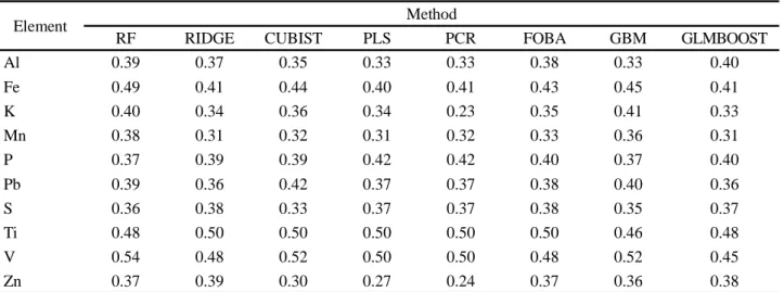
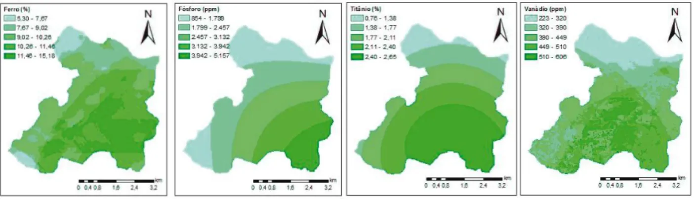
These purely spatial approaches are almost entirely based on geostatistical methods, such as kriging and co-kriging, with one of their problems being the artificial boundaries they establish on the map (MCBRATNEY et al., 2003). Such artificial boundaries were seen in this work, especially for those elements whose spatial variables were the most relevant, appearing either exclusively or in the top positions, such as Ti and P in the 0-10 cm layer and S in the 10-30 cm layer (Figure 1 and 2).
When other non-spatial predictor variables are inserted, these limits are softened, as in the case of Fe and V at 0-10 cm (Figure 1) and Ti at 10-30 cm (Figure 2). The satisfactory R² values, ranging from 0.38 to 0.54 (0-10 cm) and from 0.32 to 0.62 (10-30 cm), show the relevance of considering these relationships in predictions and associating them with the terrain attributes.
In this study, the terrain attributes considered as most relevant predictor variables were: Terrain Surface Convexity (Al at 0-10 cm); Valley Depth (Al, Mn and Zn at 0-10 cm, and Ca and P at 10-30 cm); Real Surface Area (Al at 0-10 cm, and Ca, Fe and Pb at 10-30 cm); Terrain Surface Texture (K, Mn and V at 0-10 cm); Diurnal Anisotropic (K and S at 0-10 cm); Convergence Index (K at 0-10 cm, and Fe, Cr and K at 10-30 cm); Standardized
Figure 1 - Total iron (Fe2O3), phosphorus (P2O5), titanium (TiO2) and vanadium (V2O5) content using Ridge Regression (Ti), Partial Least Squares (P) and Random Forest (Fe and V)
Height (Mn at 0-10 cm); Mid Slope Position (Mn and Zn at 0-10 cm, and Ca and K at 10-30 cm); Topographic Wetness Index (Mn and Zn at 0-10 cm, and Ca, K, Pb and Zr at 10-30 cm); Slope Height (Pb at 0-10 cm); Diffuse Insolation1 (Al and S at 0-10 cm, and Al, Cr and P at 10-30 cm); Direct to Diffuse Ratio1 (S at 0-10 cm); Surface Specific Points (Cr at 10-30 cm); Slope (Fe, Pb at 10-30 cm) and MDE (S at 10-30 cm). In the literature, studies can be found that test MDE-derived variables as predictors for generating digital maps using different methods (MENEZES et al., 2014; OLIVEIRA et al., 2012; PINHEIRO et al., 2012; RYAN et al., 2000; YANG et al., 2016).
CONCLUSIONS
1. The Random Forest algorithm was superior to the other models in predicting the chemical attributes of the soil at both depths, especially at the depth of 10-30 cm, with superior R² values for seven elements, and is therefore suggested for predicting soil attributes in the region of the study;
2. Spatial variables proved to be essential for predicting soil attributes and should be considered when modelling chemical elements in the soil;
3. It is possible to predict Al, Ca, Cr, Fe, K, Mn, P, Pb, S,
Ti, V, Zn and Zr with an R2 ranging from 0.32 to 0.62 by
the methods tested.
REFERENCES
ADHIKARI, K. et al. Digital mapping of soil organic carbon contents and stocks in Denmark. Plos One, v. 9, n. 8, p. e105519, 2014.
AKPA, S. I. C. et al. Total soil organic carbon and carbon sequestration potential in Nigeria. Geoderma, v. 271, p. 202-215, 2016.
Figure 2 - Total sulfur (SO3) and titanium (TiO2) content using Partial Least Squares (S) and Generalized Boosted Regression Models (Ti)
ALVES, E. E. N. et al. Determinação da massa por área mínima de amostras de solo e vegetal para análise no µ-EDX.
In: SIMPÓSIO MINEIRO DE CIÊNCIA DO SOLO, 3., 2015,
Viçosa, MG. Anais [...]. Viçosa, MG: UFV, 2015. p. 28-30. ARRUDA, G. P. de; DEMATTÊ, J. A. M.; CHAGAS, C. da S. Mapeamento digital de solos por redes neurais artificiais com base na relação solo-paisagem. Revista Brasileira de Ciência do Solo, v. 37, p. 327-338, 2013.
BISHOP, T. F. A. et al. Modelling soil attribute depth functions with equal-area quadratic smoothing splines. Geoderma, v. 91, n. 1/2, p. 27-45, 1999.
BÖHNER, J.; MCCLOY, K. R.; STROBL, J. SAGA: analysis and modelling applications. Göttingen: Göttinger Geographische Abhandlungen, 2006. 130 p.
CAMERA, C. et al. A high resolution map of soil types and physical properties for Cyprus: a digital soil mapping optimization. Geoderma, v. 285, p. 35-49, 2017.
CHAGAS, C. da S. et al. Spatial prediction of soil surface texture in a semiarid region using random forest and multiple linear regressions. Catena, v. 139, p. 232-240, 2016.
DAVIES, B. E.; GAMM, S. A. Trend surface analysis applied to soil reaction values from Kent, England. Geoderma, v. 3, p. 223-231, 1969.
DHARUMARAJAN, S. et al. Spatial prediction of major soil properties using Random Forest techniques: a case study in semi-arid tropics of South India. Geoderma Regional, v. 10, p. 154-162, 2017.
GOMEZ, C. et al. Soil organic carbon prediction by hyperspectral remote sensing and field vis-NIR spectroscopy: an australian case study. Geoderma, v. 146, n. 3/4, p. 403-411, 2008. GRIMM, T. et al. Soil organic carbon concentrations and stocks on Barro Colorado Island: digital soil mapping using Random Forests analysis R. Geoderma, v. 146, p. 102-113, 2008. GROENEVELD, R. A.; MEEDEN, G. Measuring skwness and kurtosis. Jounal of the Royal Statistical Society, v. 33, n. 4, p. 391-399, 1984.
GUO, P-T. et al. Digital mapping of soil organic matter for rubber plantation at regional scale: an application of random forest plus residuals kriging approach. Geoderma, v. 237-238, p. 49-59, 2015.
HENGL, T. et al. Mapping soil properties of Africa at 250 m resolution: Random Forests significantly improve current predictions. Plos One, v. 25, p. 1-26, 2015.
HEUVELINK, G. B. M. et al. Geostatistical prediction and simulation of European soil property maps. Geoderma Regional, v. 7, n. 2, p. 201-215, jun. 2016.
KABATA-PENDIAS, A. Trace elements in soils and plants. 4. ed. New York: CRC, 2010. 533 p.
KISS, J. J. et al. The distribution of fallout Cesium-137 in southern Saskatchewan, Canada. Journal of Environmental Quality, v. 17, p. 445-452, 1988.
LAGACHERIE, P. Digital soil mapping: a state of the art. In: HARTEMINK, A. E.; McBRATNEY, A. B.; MENDONÇA-SANTOS, M. de L. Digital soil mapping with limited data. New York: Springer, 2008. cap. 1, p. 3-14.
LIMA, J. S. de S. et al. Análise espacial de atributos químicos do solo e da produção da cultura pimenta-do-reino (piper nigrum, l.). Idesia, v. 28, n. 2, p. 31-39, 2010.
MA, Y. et al. Mapping key soil properties to support agricultural production in Eastern China. Geoderma Regional, v. 10, p. 144-153, 2017.
MALONE, B. P. et al. Using model averaging to combine soil property rasters from legacy soil maps and from point data. Geoderma, v. 232/234, p. 34-44, 2014.
McBRATNEY, A. B. et al. On digital soil mapping. Geoderma, v. 117, n. 2, p. 3-52, 2003.
MENEZES, M. D. et al. Solum depth spatial prediction comparing conventional with knowledge-based digital. Scientia Agricola, v. 71, n. 4, p. 316-323, 2014.
OLIVEIRA, S. et al. Modeling spatial patterns of fire occurrence in Mediterranean Europe using multiple regression and Random Forest. Forest Ecology and Management, v. 275, p. 117-129, 2012.
PINHEIRO, H. S. K. et al. Modelos de elevação para obtenção de atributos topográficos utilizados em mapeamento digital de solos. Pesquisa Agropecuária Brasileira, v. 47, n. 9, p. 1384-1394, 2012.
POGGIO, L. et al. Regional scale mapping of soil properties and their uncertainty with a large number of satellite-derived covariates. Geoderma, v. 209/210, p. 1-14, 2013.
RAMIFEHIARIVO, N. et al. Mapping soil organic carbon on a national scale: towards an improved and updated map of Madagascar. Geoderma Regional, v. 9, p. 29-38, 2017. ROUSE J. W. et al. Monitoring the vernal advancement and retrogradation (Green wave effect) of natural vegetation. Greenbelt: National Aerospace Spatial Adminitration, 1973. 371 p. RUSSELL, J. S.; MOORE, A. W. Comparison of different depth weightings in the numerical analysis of anisotropic soil profile data. In: International Congress of Soil Science, 9., 1968, Adelaide. Transactions […]. Adelaide: ISSS, 1968. v. 4, p. 205-2013. 1968.
RYAN, P. J. et al. Integrating forest soils information across scales: spatial prediction of soil properties under Australian forests. Forest Ecology and Management, v. 138, p. 139-157, 2000.
SREENIVAS, K. et al. Digital mapping of soil organic and inorganic carbon status in India. Geoderma, v. 269, p. 160-173, 2016. VÅGEN, T-G. et al. Mapping of soil properties and land degradation risk in Africa using MODIS reflectance. Geoderma, v. 263, p. 216-225, 2016.
VAYSSE, K.; LAGACHERIE, P. Evaluating digital soil mapping approaches for mapping GlobalSoilMap soil properties from legacy data in Languedoc-Roussillon (France). Geoderma Regional, v. 4, p. 20-30, 2015.
WIESMEIER, M. et al. Digital mapping of soil organic matter stocks using Random Forest modeling in a semi-arid steppe ecosystem. Plant Soil, v. 340, p. 7-24, 2011.
YANG, R-M. et al. Comparison of boosted regression tree and random forest models for mapping topsoil organic carbon concentration in an alpine ecosystem. Ecological Indicators, v. 60, p. 870-878, 2016.