Digital Soil Mapping Using Machine Learning Algorithms in a Tropical Mountainous Area

* Corresponding author:

E-mail: elianadsouza@yahoo.com.br

Received: January 6, 2018

Approved: July 30, 2018

How to cite: Meier M, Souza E, Francelino MR, Fernandes Filho EI, Schaefer CEGR. Digital soil mapping using machine learning algorithms in a tropical mountainous area. Rev Bras Cienc Solo. 2018;42:e0170421.

https://doi.org/10.1590/18069657rbcs20170421

Copyright: This is an open-access article distributed under the terms of the Creative Commons Attribution License, which permits unrestricted use, distribution, and reproduction in any medium, provided that the original author and source are credited.

Digital Soil Mapping Using Machine

Learning Algorithms in a Tropical

Mountainous Area

Martin Meier(1)

, Eliana de Souza(1)*

, Marcio Rocha Francelino(2)

, Elpídio Inácio Fernandes Filho(2)

and Carlos Ernesto Gonçalves Reynaud Schaefer(2)

(1)

Universidade Federal de Viçosa, Departamento de Solos, Programa de Pós-Graduação em Solos e Nutrição de Plantas, Viçosa, Minas Gerais, Brasil.

(2)

Universidade Federal de Viçosa, Departamento de Solos, Viçosa, Minas Gerais, Brasil.

ABSTRACT: Increasingly, applications of machine learning techniques for digital soil mapping (DSM) are being used for different soil mapping purposes. Considering the variety of models available, it is important to know their performance in relation to soil data and environmental variables involved in soil mapping. This paper investigated the performance of eight machine learning algorithms for soil mapping in a tropical mountainous area of an official rural settlement in the Zona da Mata region in Brazil. Morphometric maps generated from a digital elevation model, together with Landsat-8 satellite imagery, and climatic maps, were among the set of covariates to be selected by the Recursive Feature Elimination algorithm to predict soil types using machine learning algorithms. Mapping performance was assessed using the confusion matrix, and the Z-test among the Kappa indexes of the matrices. In a conventional soil survey, the soils described and classified in the Brazilian System of Soil Classification [Argissolos Vermelho-Amarelos Distróficos – PVAd (Acrisols), Cambissolos Háplicos Tb Distróficos - CXbd (Cambisols),

Gleissolos Háplicos Háplicos Tb Distróficos - GXbd (Gleysols), Latossolos Amarelos Distróficos - LAd (Xanthic Ferralsos), Latossolos Vermelho-Amarelos Distróficos - LVAd (Rhodic Ferralsols), and Neossolos Litólicos Distróficos - RLd (Neossols)] were grouped into composite mapping units (MU) using the conventional method. The eight algorithms showed similar performance without statistical difference (Kappa 0.42-0.48). The mapping of soils with varying slopes (LAd, LVAd, CXbd) showed lower accuracy, whereas soils on hydromorphic lowlands (GXbd) were classified more accurately. In map algebra, the result was rather satisfactory, with 63-67 % agreement between the conventional soil map and maps produced by machine learning. The areas with the largest disagreement in the DSM occurred in the LAd unit due to subtle color variation in the Latossolos mantle without a clear relation to any environmental variable, highlighting difficulties in DSM regarding hill slope landforms. Model performance was satisfactory, and good agreement with the conventional soil map demonstrates the importance of the DSM as a potential complementary tool for assisting soil mapping in mountainous areas in Brazil for the purpose of land use planning.

Keywords: soil classification, machine learning, pedometrics, land use planning, agrarian reform.

INTRODUCTION

Soil mapping is key for guiding decision makers in natural resource assessments, environmental modelling, and land use studies. The soil mapping process requires the knowledge and experience of a senior pedologist for the stages of soil surveying, soil classification, and soil mapping (Kempen et al., 2012; Resende et al., 2014). For mapping soils, the pedologist makes use of environmental information, such as climate, lithology, vegetation, and landforms; analyses and interpretations of soil samples collected in the area of interest; and consideration of all elements involved in soil-landscape dynamics (Nolasco-Carvalho et al., 2009; Brady and Weil, 2013; Schaefer, 2013). Through a systematic analysis of field observation and supporting data during the mapping, the pedologist identifies the relationships between soils and landscape features and establishes the soil mapping unit boundaries to be drawn on the map (Nolasco-Carvalho et al., 2009; Brevik et al., 2016).

The Digital Soil Mapping (DSM) technique has shown great potential in producing spatial information (McBratney et al., 2003). Basically, the DSM allows maps of soil spatial distribution to be created by means of numerical models that take soil environmental covariates into account, allowing inferences to be made of spatial and temporal variations of soil types and their properties (Lagacherie and McBratney, 2007). Digital Soil Mapping studies make use of spatially dense maps of covariates, related to soil formation and processes, that are usually available.

Due to DSM’s increasing popularity, the number of models and the procedures for optimizing modelling performance has increased (Minasny and McBratney, 2016). Some models applied to soil mapping include the following: geostatistical (Kempen et al., 2012); fuzzy membership (Nolasco-Carvalho et al., 2009; Taghizadeh-Mehrjardi et al., 2015; Rizzo et al., 2016); and Clorpt techniques based on environmental correlation, usually applying Artificial Neural Networks - ANNs, CART, and regression models (Brungard et al., 2015; Heung et al., 2016; Chagas et al., 2017).

In a recent review on the use of DSM for soil mapping in Brazil (ten Caten et al., 2012), the approaches used up to 2011 show three main classification models applied for DSM (ANNs, logistic regression, and decision tree). Up to then, studies had not used open source software, such as SAGA and R. In the following years, due to the development and free sharing of codes for soil modeling on open source platforms, several models run in R software became popular in research dealing with soil mapping. After 2011, Logistic regression continued to feature among the most used models for mapping soil classes in Brazil (Souza, 2013; Vasques et al., 2015; Chagas et al., 2017; Jeune et al., 2018), along with the following: ANNs (Arruda et al., 2016), maximum likelihood (Demattê et al., 2016), fuzzy logic and expert knowledge (Silva et al., 2014), and tree-based models (Bazaglia Filho et al., 2013; Höfig et al., 2014; Rizzo et al., 2016).

The aim of this paper was to investigate the performance of machine learning algorithms on soil mapping in a mountainous area of the Zona da Mata region, state of Minas Gerais, Brazil. The main objectives were: 1) to perform soil mapping on a 1:50,000 scale using a conventional method to serve as a reference map for comparison with soil maps of DSM models; 2) to select the most relevant set of environmental covariates to generate soil class maps using machine learning algorithms; and 3) to compare machine learning algorithms for soil mapping in a hilly, dissected tropical landscape.

MATERIALS AND METHODS

Study area

The present study was carried out in the area of the Dênis Gonçalves Settlement of Agrarian Reform (21° 34’ 30” S and 43° 12’ 33” W, and 21° 39’ 36” S and 43° 09’ 15” W), with a total area of 4,213.60 hectares. The area occupies lands in the municipalities of Goianá, Chácara, Coronel Pacheco, and São João Nepomuceno, located in the mesoregion of the Zona da Mata of the Minas Gerais State, Brazil (Figure 1) from 409 to 928 m altitude.

The climate in the region is classified as Cwb (Köppen classification system), subtropical, and mesothermic, with mild summers, and rainfall concentrated from October to April, and cold and dry winters (May to September) (Alvares et al., 2013). The mean annual temperature is 18.7 °C, and mean annual rainfall is 1,528 mm. It is located in the Atlantic Forest biome, formerly a semi-deciduous forest area. Two main rivers cross through the settlement: the Cágado River, in the southern part of the border

Figure 1. Localization of the soil pits used for soil classification in the Dênis Gonçalves Settlement, Mesoregion of the Zona da Mata

region, Minas Gerais, Brazil.

21° 37’ 30” S

43° 15’ 0” W

São João Nepomuceno Chácara

Soil pit

Complete morphological description and sampling

Characterization and classification Coronel

Pacheco

Goianá N

Brazil

Minas Gerais

Zona da Mata 2 km

1 0

43° 12’ 30” W 43° 10’ 0” W

21° 35’ 0”

between the municipalities of Chácara and São João Nepomuceno, and the Rio Novo, in the northern parts of the lands of Coronel Pacheco and Goianá, all part of the Paraíba do Sul basin.

The settlement is split along the middle by a group of mountains named “Serra da Babilônia”, which forms three distinct environments: the first one, the “Serra”, with rocky outcrops steep in the east-west direction. This is a typical structural environment, favoring the emergence of a truncated hydrography in the southern part. Towards the north, the landscape is dominated by low hills(morrotes) with gently rolling to rolling slopes and elongated valley bottoms, dominated by meandering streams that create hydromorphic environments dominated by Gleysols. The third environment is located to the south of the mountain range, with predominance of high, mountainous topography and flat valley bottoms, embedded, and elongated. These landscapes are characteristic of the Zona da Mata region, which usually has low fertility soils covered with pastures, coffee fields, and forests (Resende et al., 2014) and highly dissected landscapes of the “mares de morros” (sea-of-hills) (Ab’Sáber, 1975; Silva and Mello, 2011). In this area, rivers generally have terraces and alluvial plains (Silva and Mello, 2011; Schaefer, 2013; Resende et al., 2014).

Soil survey and soil mapping unit composition

A total of 20 soil pits were opened for complete morphological description and sample collection. Additionally, 124 pits (extra samples) were collected (mini-pits and auger samples), characterized, and classified, for a total of 144 sites of soil sampling and description (Figure 1). The soils were surveyed in a systemic way throughout the area, considering the existing tracks and roads within the geoenvironments, stratified by a senior pedologist. In addition, the settlement was stratified into regions according to knowledge obtained from settler families (Table 1).

Soil sampling and description was carried out according to the IBGE (2015). To define the sampling sites, the area was stratified into geoenvironmental units (lowlands and terraces, hydromorphic plains, upland tops, and colluvial slopes).

The soil samples were subjected to physical and chemical analyses according to Claessen (1997) and classified at the third level of classification, according to the Brazilian Soil Classification System - SiBCS (Santos et al., 2013).

Table 1. Soil classes and number of soil pits surveyed per class in the Dênis Gonçalves settlement

Soil Class/Taxa SiBCS(1) Soil Class/Taxa

(WRB - IUSS)(2)

Soil pit Full

profile sampleExtra Total CXbd - Cambissolos Háplicos Tb

Distróficos Dystric Cambisols 5 33 38

GXbd - Gleissolos Háplicos Tb

Distróficos Gleysols 1 17 18

LAd – Latossolos Amarelos Distróficos Xanthic Ferralsols 9 22 31

LVAd - Latossolos Vermelho-Amarelos

Distróficos Rhodic Ferralsols 3 20 23

PVAd - Argissolos Vermelho-Amarelos

Distróficos Rhodic Acrisols 2 17 19

RLd - Neossolos Litólicos Distróficos Neosols - 15 15

Total 124

The mapping units (MUs) were defined by grouping areas of soils on a 1:50,000 scale, according to the Technical Handbook of Pedology (IBGE, 2015). The MUs were delineated using visual interpretation of the soil pattern distribution in the area. Soil-landscape relationships were established using visual interpretation of field observations, soil descriptions, and the following subsidiary maps: 1) satellite imagery (GeoEye sensor obtained from the Google Earth platform, with spatial resolution of 0.41 m); 2) digital elevation model - DEM [generated from Advanced Land Observing Satellite (ALOS) images with 12.5 m of spatial resolution]; and 3) maps derived from the DEM (i.e., slope, elevation, solar radiation, aspect).

Covariates used for digital soil mapping - DSM

A set of 73 covariates related to soil formation factors were used on DSM models. The data were obtained from the following freely available databases:

• Orbital images, with 5 m spatial resolution, obtained from the Google Earth platform (Google, 2016), were used for mapping the stream. The Euclidean distance from the drainage network (eddrainage) was calculated;

• Map of soil units on a 1:650,000 scale (FEAM/UFV/SEMA, 2010);

• Geological map on a 1:100,000 scale (Delgado et al., 2013);

• Bioclimatic variables (BIO01, BIO02,…, BIO19) from nineteen maps derived from monthly temperature and rainfall data of WorldClim – Global Climate Data (Fick and Hijmans, 2017);

• Spectral imagery of the Landsat-8 satellite, acquired on October 11, 2015: band 1 (430-450 nm), band 2 (450-510 nm), band 3 (530-590 nm), band 4 red (640-690 nm), band 5 near infrared (850-880 nm), band 6 SWIR1 (1570-1650 nm), band 7 SWIR2 band (2110-2290 nm), band 8 panchromatic band (500-680 nm), band 9 Cirrus (1360-1380 nm), band 10 thermal infrared band TIRS1 (10600-11190 nm), and band 11 thermal infrared band TIRS2 (11500-12510 nm), (USGS archives, path/row = 217/75);

• Digital elevation model (DEM) of the Alos Palsar imagery (Advanced Land Observing Satellite - Phased Array type L-band Synthetic Aperture Radar), with spatial resolution of 12.5 meters [Japan Aerospace Exploration Agency - Alos Palsar (2016)], was used to derive a total of 40 morphometric maps of covariates. The following covariates were generated using the RSaga package (Brenning et al., 2018): aspect, convergence index, curvature of cross section, curvature of flow line, general curvature, longitudinal curvature, maximum curvature, minimal curvature, flat curvature, profile of curvature, tangential curvature, total curvature, curvature classified, hydrological gradient, diurnal anisotropic heating, difference of hydrological gradient, mass balance index (balance between erosion and deposition), elevation above the sea level, mid-slope position, multi-resolution index of valley bottom flatness (MRVBF), normalized height, real surface area, slope, slope height, diffuse solar radiation 1 (January), diffuse solar radiation 2 (June), direct solar radiation 1 (January), direct solar radiation 2 (June), duration of radiation 1 (January), duration of radiation 2 (June), total solar radiation 1 (January), total solar radiation 2 (June), standardized height, surface of specific points, terrain ruggedness index, convexity of surface, texture of surface, valley depth, terrain ruggedness, and topographic wetness index (TWI).

Selection of covariates for digital soil mapping

We used a selection process where the covariates were ranked based on their importance, selecting the top ten with highest importance for soil mapping. The selection procedure was performed by using the Recursive Feature Elimination (RFE) algorithm, implemented on the Caret Package (Kuhn, 2017), combined with correlation analyses for removal of covariates with 95 % or higher correlation with others.

Recursive Feature Elimination is an algorithm that performs a backward selection, which avoids refitting many models at each step of the search (Kuhn and Johnson, 2013). When the full model is created, a measure of variable importance is computed and shows the ranks of predictors from most to least important (Kuhn, 2013). In this study, we used the Random Forest based RFE, which ranks the predictors based on the Gini index, as implemented in the Random Forest algorithm (Breiman, 2001).

The selection was run in two phases: the first, in which the highly correlated covariates were identified and the ones with the highest correlation removed (Kuhn, 2017), and the second, in which an importance rank was determined by RFE, allowing selection of the most important ones. In the first phase, categorical covariates were left out, and continuous ones were used in a pair-wise analysis that was run using the ‘findcorrelation’ function, as implemented in the Caret Package (Kuhn, 2017) to determine the correlation among covariates without their being assessed in a prediction model. A correlation matrix was generated, and the absolute values of pair-wise correlations were considered in the analyses. In these analyses, if two covariates have a high correlation, the function looks at the mean absolute correlation of each covariate and removes the covariate with the largest mean absolute correlation. A threshold value greater than or equal to 98 % was established as the critical value for the covariate to be removed. Once the dataset had been reduced by removing highly correlated covariates, the RFE procedure was run, establishing 10 as the maximum number of covariates to be left in the model.

Recursive Feature Elimination algorithm selection is an iterative process that eliminates the least important predictors from the model based on an initial measure of predictor importance (Kuhn and Johnson, 2013). We selected Random Forest as the base model for running the RFE. First, a full Random Forest model is created using all covariates, and a measure of covariate importance is computed to rank the covariates from most to least important. Secondly, the Random Forest model is tuned and trained iteratively with the most important covariates and without the least important ones until only 10 covariates remain.

Machine Learning Algorithms

Eight algorithms were assessed: Random Forest (RF), Extreme Gradient Boosting (xgBoost), Ranger Random Forest (Ranger), Weighted Subspace Random Forest (WSRF), Support Vector Machine with Linear Kernel (SVMLinear), Support Vector Machine with Polynomial Kernel (SVMPoly), Bagged AdaBoost (AdaBag), and Extra Trees - Random Forest by randomization (ExtraTree). All algorithms were implemented in the Caret package (Kuhn, 2013) and run on the R program (R Development Core Team, 2016) using the available parameters.

Random Forest (Ranger), Weighted Subspace Random Forest (WSRF), Random Forest by randomization (Extra Trees)

Random Forest (RF) is a general term used for a set of “tree-based” classifiers. The method was developed as an extension to the regression tree classifier (CART) to improve model performance (Breiman, 2001) and applied to predictions of discrete and categorical variables.

used. The number of predictors used in the construction of each tree and the number of trees to be constructed in the forest vary, depending on the dataset (Liaw and Wiener, 2018). Each tree is constructed from samples selected from the total dataset by using the bootstrap method (Efron and Gong, 1983). This selection allows more robust error estimates with a second set of samples, called Out-of-Bag (OOB), also selected from the total dataset by the bootstrap and excluded from the prediction.

Variant models have been developed from the principle of RF operation [e.g., Ranger (Wright and Ziegler, 2015; Wright, 2017), WSRF (Meng et al., 2012), and ExtraTrees (Simm and Abril, 2014)]. Ranger has shown to be efficient in soil nutrient mapping on an ensemble model by Hengl et al. (2017a) and in soil properties by Hengl et al. (2017b).

The Weighted Subspace Random Forest (WSRF) is an algorithm that can classify large datasets using a mechanism similar to RF, but applied to small subsets. It is a new method of weighting variables used in sample selection, rather than using the traditional method of random selection. This new approach is particularly useful in models using large dimension datasets (Meng et al., 2012). However, the error effect of setting the weights when using low dimension datasets is substantial and may result in poor performance of the model (Li and Zhao, 2009).

The use of ExtraTree (Extremely Randomized Trees) is similar to RF. The difference is that whereas each branch of the forest in RF chooses the best cut-off threshold for categorical values, ExtraTree chooses the cut-off value (evenly) randomly. However, like RF, the categorical data with the highest gain (or better score) is chosen after the cutoff limit is set (Simm and Abril, 2014).

Support Vector Machine (with Linear Kernel/with polynomial Kernel)

The Support Vector Machine (SVM) algorithm, introduced by Cortes and Vapnik (1995), performs a binary classification. The basic idea of the model is to find a hyperplane that best separates the points of two classes by maximizing the margin between those points of both classes that are closest to each other, called support vectors. The SVM function can easily work with non-linear patterns by transforming the original data into new features, which is a basic characteristic of the kernel function. This hyperplane from the maximized margins is used as a criterion for subsequent classification (Kuhn, 2013).

The SVM has been applied to soil mapping due to its ability to handle large datasets, learning complex data-classes and making decisions regarding separation, and also because it is based on traditional statistical methods applied to pedometric studies (Brungard et al., 2015; Brevik et al., 2016; Heung et al., 2016; Forkuor et al., 2017). In addition, the SVM performs well in low-dimension datasets and has high power for generalizing information (Li and Zhao, 2009).

To run the SVM, we used the kernlab package (Karatzoglou et al., 2016). The SVM with radial basis function (SVMRadial) uses machine learning and kernel functions for pattern recognition.

Bagged AdaBoost (AdaBag)

AdaBag is an algorithm that makes possible to implement two popular tree-based models: boosting and bagging. The main difference between these two ensemble model methods is that boosting builds its base classifiers in sequence, updating a distribution over the training examples to create each base classifier, whereas bagging combines individual classes in repetitions of bootstrap training (Alfaro et al., 2015).

errors of the samples are increased, while the weights of the correct classifications decrease, controlling the error rate and forcing the classifier to focus on more difficult samples (Alfaro et al., 2013).

Extreme Gradient Boosting (xgBoost)

Extreme Gradient Boosting (xgBoost) is a hybrid algorithm of the tree model, applied to regression and classification predictions. It is an ensemble model that works based on prediction of the weak set, which is highly effective and widely used (Chen and Guestrin, 2016). Its scalable working mechanism is based on stages with increases in the number of trees. A differential aspect of the model is its ability to handle sparse data. On soil science, the model has been applied to mapping soil nutrients (Hengl et al., 2017a) and soil properties in the United States (Ramcharan et al., 2018).

The model is optimized by adjusting parameters, such as the number of interactions, the maximum number of tree branches, the multiplication parameters of tree shrinkage after each interaction, reduction in the influence of each tree, the amount of space for future trees, minimum number of weighted input features, the sum of the instances, and the percentage of samples for sampling (Chen et al., 2017). The model is trained in an additive way, using learned patterns to redefine the parameters (Chen and Guestrin, 2016).

Model training and evaluation

The soil taxonomic classes described at 144 sites (Table 1) were used as the dataset for training and validating the models. The number of soil sites per MU was as follows: CXbd (38), GXbd (18), LAd (31), LVAd (23), PVAd (19), and RL (15). Six MUs with a single soil component were defined within the settlement area for the soil mapping using machine learning. This soil mapping approach followed the guideline for a 1:50,000 scale of soil mapping, considering the detail of spatial information and the soil survey approach (IBGE, 2015).

Model training used 10-fold cross-validation repeated 5 times. This method is suggested as the most weighted in evaluation of model performance when the datasets are not large enough to be split into training and external validation samples (Kuhn, 2013).

To evaluate the performance of the algorithms for soil mapping, the confusion matrix was used to derive the Kappa indexes and the overall accuracy. The matrix is constructed using a discrete multivariate technique to evaluate thematic accuracy (Congalton and Green, 2009). The Kappa coefficient (K) is a measure of actual agreement minus chance agreement. In other words, it is a measure of how much the classification data agrees with the reference data, and it can be calculated as follows:

K = n Σ

c

i=1nii – Σ c

i=1 ni+ + n+i

n2 – Σc

i=1ni+ + n+i

Eq. 1

in which K is the estimate of the Kappa; nii is the value in row i and column i; ni+ is the sum of line i, and n+i is the sum of column i of the confusion matrix; n is the total number of samples; and c is the total number of classes. The Kappa index ranges from 0 to 1, and performance is considered moderate for values between 0.20-0.60 (Landis and Koch, 1977).

To perform a statistical analysis for detecting difference between the Kappa obtained by the algorithms, when mapping the soil, we used the Z-test, which compares pairs of algorithms according to the following equation:

Z = |K1 – K2|

√

In which Z is the value that defines the test, K1 and K2 are the Kappa values of algorithms 1 and 2 taken for the comparison; and “var” is the variance of Kappa algorithms 1 and 2, respectively. The Z value makes possible to evaluate the difference between classifiers in performing the mapping with the available data. The statistical significance test follows the null hypothesis considered in this study, where there is a 5 % confidence interval, with a Z value greater than 1.96, which is significant (Congalton and Green, 2009).

Variability of Mapping Units among DSM models

To identify areas in the map where the machine learnings showed greater variability in mapping the soil MUs, we analyzed the eight maps generated from the algorithms, performing zonal statistical analysis with the Zonal statistical function from the “Spatial Analyst Tools” package of the ArcGis 10.2 software. Variability analysis runs a per-pixel calculation among the soil maps to calculate the MU “Variety” (i.e., calculate the number of unique MUs at each pixel). If the classifiers agree on mapping a MU at one pixel, the function returns the number one (one unique MU); for two different MUs assigned, it returns the number two, and so forth. Hence, the larger the number of classifier disagreement, the larger the mapping variability.

Analysis of agreement between conventional map and digital soil maps

Concordance analysis between the conventional soil map and the soil maps from the machine learning algorithms was performed to give a comparative measure in terms of area mapped for each MU. The soil in the conventional map was converted to a raster file and analyzed by map algebra using Boolean logic. To calculate pixel-by-pixel agreement, a concordant pixel returns the value 1 and a non-concordant one returns the value zero.

As the soil map was composed by MUs with soil associations up to three soil classes, the map was reclassified for maps of a single MU component (i.e., soil map of the first, second, and third soil class component of the MU). For each DSM map comparison, the concordance with the three maps of MU components were added up, and agreement was expressed as the area of matching soil classes on both maps.

RESULTS AND DISCUSSION

Soil mapping using a conventional method

The soils described in the settlement were classified at the third categorical level, revealing a predominance of the following classes: Argissolos Vermelho-Amarelos Distróficos (PVAd),

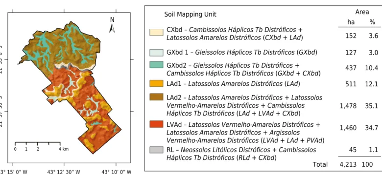
Cambissolos Háplicos Tb Distróficos (CXbd), Gleissolos Háplicos Tb Distróficos (GXbd), Latossolos Amarelos Distróficos (LAd), Latossolos Vermelho-Amarelos Distróficos (LVAd), and Neossolos Litólicos Distróficos (RLd). A total of seven MUs were formed for the soil mapping purpose (Figure 2).

Latossolos cover a large area, corroborating previous soil surveys in a nearby region (the Coronel Pacheco research station) (Santos et al., 1980), whereas Argissolos occur as inclusions or in association with Latossolos. At the hilltops, Latossolos are most developed and easily distinguishable and mapped on flat or convex slopes in the uplands. On a landscape scale, color distinction at the second level is difficult due to the small difference between the 5YR and 7.5YR; hence, we mapped associations between these

Latossolos classes (Figure 2).

In the lowlands, the typical MU is the association of Gleissolos and Cambissolos (GXbd2), identified on the satellite image with a gray pattern indicating seasonal flooding, whereas

Gleissolos (GXbd1) are found on the darkest areas of the image, indicating swampy areas of permanent waterlogging.

The areas of highland ridges on the steep slopes of the Serra da Babilônia with sparse rocky outcrops contain Neossolos Litólitcos (RL), which are associated with shallow Cambissolos, since soils in these areas are difficult to map separately due to the scale adopted (1:50,000).

Covariates selected for soil mapping using machine learning

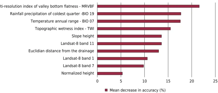
The ten covariates selected for soil mapping, ranked by importance, were as follows: 4 morphometric covariates (slope height, standardized height, TWI, and MRVBF); 3 images from Landsat-8 (bands 1, 7, and 11); two climatic maps [rainfall of the coldest trimester (BIO19) and the annual temperature range (BIO07), which stands for the maximum temperature of the warmest month, minus the minimum temperature of the coldest month]; and the map of Euclidean distance from the drainage network (eddrainage). The high number of covariates related to landform is due to the influence of relief on the soil formation process in the area, where topography and landform are key factors for soil diversity.

The contribution of each covariate to the soil-mapping model (Figure 3), measured as the percentage of decreasing accuracy, highlights the morphometric covariates as highly important in mapping soil distribution in the study area. The Multi-resolution index of valley bottom flatness (MRVBF) is the most important, contributing 21.6 %. The TWI contributed 15.5 % and slope height 13.6 %. The two bioclimatic covariates, related to temperature and rainfall, scored around 17.5 % each, and were the second more important. The covariates selected were derived from a large variety of sources (Figure 3), including spectral information from satellite imagery, Euclidian distance from the drainage network, and bioclimatic and morphometric sources.

Evaluation of soil mapping with machine learning algorithms

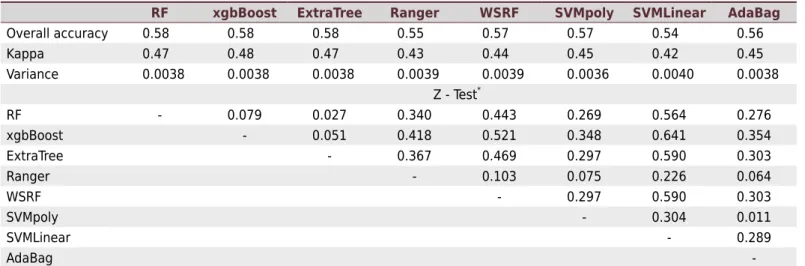
Soil mapping using the machine learning algorithms exhibited a Kappa index ranging from 0.42 to 0.48 and an overall accuracy ranging from 0.54 to 0.58 (Table 2), which can

21° 37’ 30” S

43° 15’ 0” W

RL – Neossolos Litólicos Distróficos + Cambissolos Háplicos Tb Distróficos (RLd + CXbd)

Soil Mapping Unit N

Area

ha %

152 3.6

127 3.0

437 10.4

511 12.1

1,478 35.1

1,460 34.7

45 1.1

4,213 100 Total

43° 12’ 30” W 43° 10’ 0” W

4 km 2

1 0

21° 35’ 0” S

CXbd – Cambissolos Háplicos Tb Distróficos +

Latossolos Amarelos Distróficos (CXbd + LAd)

GXbd 1 – Gleissolos Háplicos Tb Distróficos (GXbd)

GXbd2 – Gleissolos Háplicos Tb Distróficos +

Cambissolos Háplicos Tb Distróficos (GXbd + CXbd) LAd1 – Latossolos Amarelos Distróficos (LAd)

LAd2 – Latossolos Amarelos Distróficos + Latossolos Vermelho-Amarelos Distróficos + Cambissolos Háplicos Tb Distróficos (LAd + LVAd + CXbd)

LVAd – Latossolos Vermelho-Amarelos Distróficos +

Latossolos Amarelos Distróficos + Argissolos Vermelho-Amarelos Distróficos (LVAd + LAd + PVAd)

Figure 2. Conventional soil map showing the distribution of soil mapping units (MUs) and their areas of occurrence in the Dênis

be considered moderate (Landis and Koch, 1977). Overall, the xgBoost showed better performance, with a higher Kappa (0.48). It had low performance in mapping Latossolos Vermelho-Amarelos (39 %) and high performance in mapping Gleissolos (85 %). The ExtraTree, in contrast, was less accurate in mapping Argissolos (41 %) but showed high performance in mapping Gleissolos (94 %), like the RF, which mapped Gleissolos with 94 % accuracy.

The RF algorithm showed low efficiency in mapping CXbd (28 % accuracy). The MU CXbd were not adequately distinguished from Latossolos (LAd and LVAd units), although CXbd has more soil data (38) than Latossolos (LAd - 31 and LVAd - 23 soil pits) (Table 2). The area mapped as Cambissolos is also larger than areas of Latossolos. When comparing the algorithms performance on mapping the LVAd, the lowest accuracy was that of the SVMPoly, with not a single classification of this soil correctly allocated to this MU (Table 2); the best performance on mapping LVAd was achieved by the ExtraTree algorithm (43 %).

Overall, the algorithms showed moderate performance in distinguishing CXbd from

Latossolos (LAd and LVAd). Conversely, all algorithms showed good performance in mapping GXbd, in which the lowest accuracy was 82 % by the AdaBag algorithm, and the highest 94 % (RF, Ranger, and ExtraTree). These results indicate that the covariates used made it difficult to distinguish some soils on dissected terrain (Table 2).

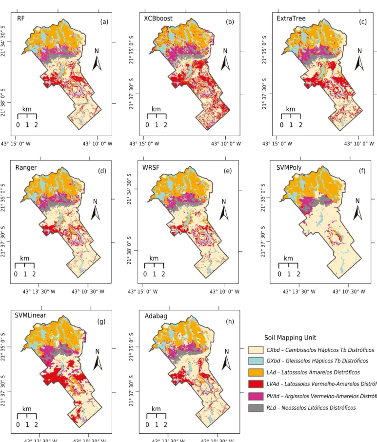
The soil maps obtained with each algorithm are shown in figure 4. In a cursive rapid visual analysis, no significant differences are noticed, except for the LVAd, which was mapped with the smallest area by the SVMPoly (Figure 4f), since the SVMPoly misclassified LVAd as CXbd (Table 2b). Similarly, confusing LVAd with CXbd occurred with all algorithms. Two MUs, CXbd, and LVAd, showed highest standard deviation in the size of area mapped (Table 3) comparing all the DSM maps, as a result of their confusing and difficult mapping. The results showed that the SVMLinear has an advantage over the SVMPoly.

Most MUs were mapped in a similar way for all algorithms, especially in the highlands, where RLd occurs (standard deviation of area mapped = 0.4 %). The MU LAd was mapped in a similar way by all algorithms, as well as GXbd, which occurs near the drainage network (Figure 4), and showed standard deviation of 0.9 %. Among algorithms, the mapping of PVAd showed more dissimilarity in its spatial distribution and mapped area in the SVMPoly mapping, which showed only 5.3 % of the area occupied by this soil type, whereas four algorithms showed a percentage of PAVd of around 8-9 % of the settlement.

0 Normalized height

Landsat-8 band 7 Landsat-8 band 1 Euclidian distance from the drainage Landsat-8 band 11 Slope height Topographic wetness index - TWI Temperature annual range - BIO 07 Rainfall precipitation of coldest quarter -BIO 19 Multi-resolution index of valley bottom flatness - MRVBF

Mean decrease in accuracy (%)

25 20

15 10

5

The SVMLinear had the worst performance, which is consistent with Brungard et al. (2015), who made the same observation. In this respect, in a study performed by Heung et al. (2016), the SVMRadial was superior to the SVMLinear in models of soil mapping at the order and suborder level.

Heung et al. (2016) also compared soil mapping in great group and order level classifications in a valley area in Vancouver, Canada, using ten machine learning algorithms. The authors found that RF was among those of highest performance, along with CART and the SVMRadial. In their study, Multinomial Logistic Regression (MLR) showed lower overall accuracy (0.42) than RF (0.63) for soil orders. Therefore, statistical difference was not investigated. Only Jeune et al. (2018) reported a statistical difference in Kappa in soil Table 2. Confusion matrixes of soil mapping with each machine learning algorithm

LAd CXbd LVAd PVAd GXbd RL Total LAd CXbd LVAd PVAd GXbd RL Total

Random Forest AdaBag

LAd 24 6 4 5 0 0 39 22 3 4 5 1 0 35 CXbd 5 19 13 2 0 5 44 6 24 15 3 1 6 54 LVAd 0 5 6 1 0 0 13 0 4 5 1 0 0 11 PVAd 1 1 0 8 1 1 12 3 2 0 7 1 1 13 GXbd 0 2 0 1 17 0 20 0 2 0 1 15 0 18 RL 0 4 0 2 0 9 15 0 3 0 2 0 8 13 Total 31 38 23 19 18 15 144 31 38 23 19 18 15 144 Acc. (%) 77 50 28 43 94 58 71 62 24 35 82 55

Over. Acc. 0.58 0.58

Kappa 0.47 0.48

Support Vector Machine Poly Kernel xgBoost

LAd 22 6 4 6 1 0 38 22 4 4 4 0 0 34 CXbd 6 20 13 4 1 5 50 6 19 9 2 0 6 43 LVAd 2 6 5 1 0 0 15 1 6 10 2 0 0 19 PVAd 1 2 1 6 0 1 11 2 3 0 8 1 2 16 GXbd 0 0 0 0 16 0 16 0 1 0 1 17 0 19 RL 0 4 0 2 0 9 15 0 5 0 2 0 7 14 Total 31 38 23 19 18 15 144 31 38 23 19 18 15 144 Acc. (%) 71 52 23 29 89 60 70 51 43 41 94 47

Over. Acc. 0.54 0.58

Kappa 0.42 0.47

Support Vector Machine - Linear Kernel ExtraTree

LAd 22 7 4 6 0 0 39 22 6 4 6 0 0 38 CXbd 6 20 14 3 0 6 49 6 19 14 1 0 5 46 LVAd 0 5 5 1 0 0 11 1 5 5 1 0 0 11 PVAd 2 0 0 6 2 0 10 1 1 0 8 1 1 12 GXbd 1 2 0 2 16 0 20 1 2 0 2 17 0 22 RL 0 4 0 2 0 8 14 0 5 0 2 0 9 16 Total 31 38 23 19 18 15 144 31 38 23 19 18 15 144 Acc. (%) 72 54 24 33 88 56 71 50 20 41 94 60

Over. Acc. 0.57 0.55

Kappa 0.45 0.44

mapping in Haiti, in which RF showed a much higher Kappa (0.55) compared to MLR (Kappa = 0.33) using external validation rather than cross-validation.

A similar study using a tree-based model (i.e., Random Forest - RF) for soil mapping in northern Iran (Pahlavan-Rad et al., 2016) applied both RF and Multinomial Regression models in mapping soils classified at the great group, subgroup, and family level and achieved highest accuracy with RF (33.9) and MLR (22.9) at the subgroup level. Similar accuracy for MLR was observed by Souza (2013) for mapping soil classes in the Rio Doce Basin, Brazil (Kappa = 0.35).

Following a different approach to obtaining soil data, Chagas et al. (2017) used legacy data extracted from a soil map for training three machine learning algorithms, obtaining highest accuracy for Random Forest (Kappa = 0.76).

The similarity in performance of machine learning algorithms observed in the present study and in the literature suggests that the performance of machine learning for soil mapping is rather similar when evaluating the Kappa index with the Z- and t-test, highlighting that the quality and robustness of datasets is of greater importance than the classifier itself. Furthermore, the number of samples per MU and the level of taxonomic classification of the soil are of key importance. As Brungard et al. (2015) pointed out, the number of pedons within each MU directly influences the accuracy of the model. Although we did not test sampling size per MU, the fact that each model scored similar Kappa for the eight models assessed, while within each model, the accuracy of the MUs did not follow the trend, indicates that for some soils the sample size should be larger in order to model their complex distribution across the landscape. In this regard, Gleissolos and Neossolos, with a limited dataset compared to LVAd, scored higher accuracy.

The number of MUs in the conventional soil map (7) differs from the DSM maps (6), as well as the number of soil components per MU. In the conventional map, there are two MUs made up of two soil components and two made up of three components, while only two MUs have a single component. In the DSM maps, all MUs are made up of a single soil component. Therefore, the MUs GXbd1 and GXbd2, and LAd1 and LAd2 on the conventional map were combined to allow better comparison with the MUs mapped with the machine learning algorithms (Table 3). The correspondence among MUs of these two mapping approaches demonstrates generalized differences in the area for most MUs due to difference in MU components. A similar area and proportion for GXbd (around 565 ha and 13.4 % of the settlement on the conventional compared to 10.7 to 12.9 % on the DSM maps). The LAd showed a 10 % increase in the area mapped by the conventional method. Cambissolos Háplicos Tb Distróficos, and for PVAd, both appear in soil associations, therefore could not be directly compared. The PVAd was not mapped as first soil component of MUs on the conventional map as its similarity to

Latossolos allows distinction only on the textural gradient of the B horizon, and CXbd was second or third component on three MUs.

The MU areas in each map and the corresponding percentages of occurrence (Table 3), show large discrepancies for two MUs. For example, the mapped area for MUs for LVAd varied from 809 ha, mapped by the xgBoost algorithm, to 42 ha, mapped by the SVMPoly. The opposite was observed for CXbd, with the smallest area mapped by xgBoost (1,332 ha) and the largest by the SVMPoly (2,166 ha). The discrepancy between these two algorithms in the mapping of LVAd and CXbd can be attributed to the SVMPoly error in mapping soils on hillslopes, as observed in the confusion matrix, where all data of LVAd was allocated to CXbd (Table 2c). Apart from these two MUs, all the remaining MUs showed low standard deviation (0.4 to 2.1 %) in their mapped area.

(Table 4). Although the tree-based algorithms (RF, Ranger, and WSRF) performed best in mapping the soils, there was no statistical difference in the mapping accuracy of these algorithms compared to binary regression models.

21° 38’ 0” S

43° 15’ 0” W 43° 10’ 0” W

21° 34’ 30” S

21° 37’ 30” S

43° 15’ 0” W 43° 10’ 0” W

21° 35’ 0” S

21° 37’ 30” S

43° 15’ 0” W 43° 10’ 0” W

21° 35’ 0” S

21° 37’ 30”

S2

1° 35’ 0”

S

43° 13’ 30” W 43° 10’ 30” W

43° 13’ 30” W 43° 10’ 30” W 43° 13’ 30” W 43° 10’ 30” W

21° 37’ 30”

S2

1° 35’ 0”

S

21° 37’ 30”

S2

1° 35’ 0”

S

21° 37’ 30”

S2

1° 35’ 0”

S

21° 38’ 0”

S2

1° 34’ 30” S

RF _(a)

N

km

0 1 2

XCBboost _(b)

N

km

0 1 2

ExtraTree _(c)

N

km

0 1 2

Ranger _(d)

N

km

0 1 2

WRSF _(e)

N

km

0 1 2

SVMPoly _(f)

N

km

0 1 2

SVMLinear

(g)

N

km

0 1 2

Adabag

(h)

N

km

0 1 2

Soil Mapping Unit

CXbd – Cambissolos Háplicos Tb Distróficos

GXbd – Gleissolos Háplicos Tb Distróficos

LAd – Latossolos Amarelos Distróficos

LVAd – Latossolos Vermelho-Amarelos Distróficos

PVAd – Argissolos Vermelho-Amarelos Distróficos

RLd – Neossolos Litólicos Distróficos

43° 15’ 0” W 43° 10’ 0” W 43° 13’ 30” W 43° 10’ 30” W

Figure 4. Maps generated by the classifiers RF (a), xgBoost (b), ExtraTree (c), Ranger (d), WSRF (e), SVMPoly (f), SVMLinear (g),

and AdaBag (h). CXbd = Cambissolos Háplicos Tb Distróficos; GXbd = Gleissolos Háplicos Tb Distróficos; LAd = Latossolos Amarelos

Distróficos; LVAd = Latossolos Vermelho-Amarelos Distróficos; PVAd = Argissolos Vermelho-Amarelos Distróficos; RLd = Neossolos

In this respect, Brungard et al. (2015) investigated the performance of eleven algorithms and reported similar accuracies for mapping soil classes in three different sites in the USA with three datasets of covariates, with no statistical difference by the T-test. In most models, the highest performance was by RF.

Mosleh et al. (2017) compared four classifiers (MLR, RF, ANNs, and Boosted regression tree) for soil mapping in Iran. The authors investigated model performance on all soil taxonomic levels, from order to family, and found out that all algorithms had the same ability at any determined taxonomic level, with better accuracy at higher taxonomic levels.

Table 3. Area of the soil mapping units in the Dênis Gonçalves settlement mapped by each machine learning classifier evaluated

and by conventional soil mapping

RF xgBoost ExtraTree AdaBag Ranger SVMLinear SVMPoly WSRF SD MU – Convent. mapping Area

MUs ha ha

CXbd 1,730 1,332 1,549 2,036 1,755 1,490 2,166 1,840 279 CXbd 152 GXbd 501 466 530 471 542 450 465 531 36 GXbd1+ GXbd2 565 LAd 970 914 929 842 999 1,083 1,103 1,034 89 LAd1 + LAd2 1,461 LVAd 433 809 602 361 289 566 42 255 238 LVAd 1,990 PVAd 347 486 363 288 380 427 223 331 81

-RLd 232 207 240 215 249 197 214 223 17 RL 46 Total 4,213 4,213 4,213 4,213 4,213 4,213 4,213 4,213 4,213

%

CXbd 41.1 31.6 36.8 48.3 41.6 35.4 51.4 43.7 6.6 CXbd 3.6 GXbd 11.9 11.1 12.6 11.2 12.9 10.7 11 12.6 0.9 GXbd1+ GXbd2 13.4 LAd 23 21.7 22.1 20 23.7 25.7 26.2 24.5 2.1 LAd1 + LAd2 34.7 LVAd 10.3 19.2 14.3 8.6 6.8 13.4 1 6.1 5.6 LVAd 47.2 PVAd 8.2 11.5 8.6 6.8 9 10.1 5.3 7.9 1.9

-RLd 5.5 4.9 5.7 5.1 5.9 4.7 5.1 5.3 0.4 RL 1.1 Total 100 100 100 100 100 100 100 100 100

SD = standard deviation of areas of MUs mapped with machine learning algorithms; CXbd = Cambissolos Háplicos Tb Distróficos;GXbd = Gleissolos

Háplicos Tb Distróficos;LAd = Latossolos Amarelos Distróficos;LVAd = Latossolos Vermelho-Amarelos Distróficos;PVAd = Argissolos Vermelho-Amarelos

Distróficos;RLd = Neossolos Litólicos Distróficos; MU - Convent. Mapping = Mapping Units of the conventional map: CXbd = Cambissolos Háplicos Tb Distróficos + Latossolos Amarelos Distróficos (CXbd + LAd); GXbd 1 = Gleissolos Háplicos Tb Distróficos (GXbd); GXbd2 = Gleissolos Háplicos Tb Distróficos + Cambissolos Háplicos Tb Distróficos (GXbd + CXbd); LAd1 = Latossolos Amarelos Distróficos (LAd); LAd2 = Latossolos Amarelos

Distróficos + Latossolos Vermelho-Amarelos Distróficos + Cambissolos Háplicos Tb Distróficos (LAd + LVAd + CXbd); LVAd = Latossolos

Vermelho-Amarelos Distróficos + Latossolos Amarelos Distróficos + Argissolos Vermelho-Amarelos Distróficos (LVAd + LAd + PVAd); RL = Neossolos Litólicos Distróficos + Cambissolos Háplicos Tb Distróficos (RLd + CXbd).

Table 4. Accuracy performance and the significance of Z-test for the kappa indexes of each classifier

RF xgbBoost ExtraTree Ranger WSRF SVMpoly SVMLinear AdaBag

Overall accuracy 0.58 0.58 0.58 0.55 0.57 0.57 0.54 0.56 Kappa 0.47 0.48 0.47 0.43 0.44 0.45 0.42 0.45 Variance 0.0038 0.0038 0.0038 0.0039 0.0039 0.0036 0.0040 0.0038

Z - Test*

RF - 0.079 0.027 0.340 0.443 0.269 0.564 0.276 xgbBoost - 0.051 0.418 0.521 0.348 0.641 0.354 ExtraTree - 0.367 0.469 0.297 0.590 0.303 Ranger - 0.103 0.075 0.226 0.064

WSRF - 0.297 0.590 0.303

SVMpoly - 0.304 0.011

SVMLinear - 0.289

AdaBag

-*

Assessment of MU variability in DSM

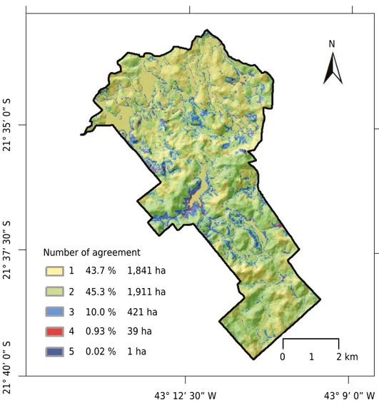
The MU variability of the eight maps, assessed pixel by pixel (Figure 5), shows agreement or disagreement among machine learning algorithms in mapping. In less than 1 % of the areas, up to five different MUs showed disagreement in mapping. The darkest colored parts of the map show areas where the algorithms most disagreed, and, conversely, the lightest colored areas indicate where the algorithms most agreed.

The number 1 (yellow) designation corresponds to areas where all algorithms agreed in classification of the MU, representing 43 % of the total settlement area, whereas the number 2 label corresponds to areas where one algorithm classified the MU differently, representing 45 % of the total area. Areas labelled 3, 4, and 5, representing 3, 4, and 5 disagreements, respectively. Together, 3, 4, and 5 comprise about 12 % of the total area and therefore indicate low variability of soil mapping by machine learning analyses in the settlement area. As can been seen in figure 5, the areas in green, disagreement occurring between two (2) MUs, are mostly the areas of LVAd that were misclassified by the SVMPoly due to confusing LVAd and CXbd. In the case of this study, we consider that the DSM models showing good agreement in mapping highlight the SVMPoly as the algorithm with the lowest performance for spatial mapping.

21° 40’ 0”

S

N

43° 12’ 30” W 43° 9’ 0” W

2 km 1

0

21° 37’ 30” S

21° 35’ 0”

S

Number of agreement

1 43.7 % 1,841 ha

2 45.3 % 1,911 ha

3 10.0 % 421 ha

4 0.93 % 39 ha

5 0.02 % 1 ha

21° 38’ 0” S

43° 15’ 0” W 43° 10’ 0” W

21° 34’ 30” S

21° 37’ 30” S

43° 15’ 0” W 43° 10’ 0” W

21° 35’ 0”

S

21° 37’ 30” S

43° 15’ 0” W 43° 10’ 0” W

21° 35’ 0”

S

21° 37’ 30”

S2

1° 35’ 0”

S

43° 13’ 30” W 43° 10’ 30” W

43° 13’ 30” W 43° 10’ 30” W 43° 13’ 30” W 43° 10’ 30” W

21° 37’ 30”

S2

1° 35’ 0”

S

21° 37’ 30”

S2

1° 35’ 0”

S

21° 37’ 30”

S2

1° 35’ 0”

S

21° 38’ 0”

S2

1° 34’ 30” S

RF

(a)

N

km 0 1 2

XCBboost (b) N ExtraTree (c) N Ranger (d) N WRSF (e) N SVMPoly (f) N SVMLinear (g) N Adabag (h) N

43° 15’ 0” W 43° 10’ 0” W 43° 13’ 30” W 43° 10’ 30” W

43° 12’ 30” W 43° 12’ 30” W 43° 12’ 30” W

km

0 1 2 0 1 2km

km

0 1 2 0 1 2 km 0 1 2 km

43° 12’ 30” W

km

0 1 2 0 1 2 km

km

0 1 2 (i) N 37 % 63 % 36 % 64 %

43° 13’ 30” W 43° 10’ 30” W

21° 37’ 30”

S2

1° 35’ 0”

S CXbd (h) GXbd1 GXbd2 LAd1 LAd2 LVAd RL Concordance Discordance 34 % 66 % 35 % 65 % 33 % 67 % 34 % 66 % 35 %

65 % 35 %

65 %

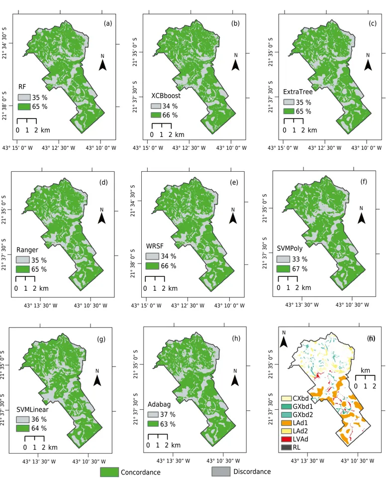
Figure 6. Map of concordance/discordance between the conventional soil map and digital soil mapping with the algorithms RF (a), xgBoost (b), ExtraTree (c), Ranger (d), WSRF (e), SVMPoly (f), SVMLinear (g), and AdaBag (h), and map of soils where discordance occurred in both mapping approaches, i.e., discordance with the conventional soil map, and discordance among the eight machine learning models (i). CXbd

= Cambissolos Háplicos Tb Distróficos + Latossolos Amarelos Distróficos (CXbd + LAd); GXbd 1 = Gleissolos Háplicos Tb Distróficos (GXbd);

GXbd2 = Gleissolos Háplicos Tb Distróficos + Cambissolos Háplicos Tb Distróficos (GXbd + CXbd); LAd1 = Latossolos Amarelos Distróficos

(LAd); LAd2 = Latossolos Amarelos Distróficos + Latossolos Vermelho-Amarelos Distróficos + Cambissolos Háplicos Tb Distróficos (LAd

+ LVAd + CXbd); LVAd = Latossolos Vermelho-Amarelos Distróficos + Latossolos Amarelos Distróficos + Argissolos Vermelho-Amarelos

Analysis of map agreement

Maps showing concordance between the conventional soil map and the maps generated by the machine learning algorithms are presented in figure 6. The results of this comparison show good agreement in gentle hilly areas and lowland landscapes. The greatest disagreements occurred in the mountainous areas with varying concave and convex slopes and steeper slopes. The proportion of agreement between machine learning mapping and conventional mapping ranged from 63 to 67 %, minored by similar spatial pattern of the maps (Figure 6).

The mapping agreements observed in this study for the eight algorithms are similar to those found by Chagas et al. (2017); they found agreement between the conventional map and DSM maps as follows: for RF, 68.7 %; for ANNs, 62.8 %; and for Decision trees, 62.3 %. The approach by Heung et al. (2016) calculated agreement based on point-observations from 262 soils extracted from a polygon map, which differs from the area-base comparison adopted in this study. Their mapping showed agreement of 72 % for RF and 63 % for the SVMLinear.

Considering the mapping scale of this study (1:50,000), we can consider the results as superior to those of Vasques et al. (2015), who compared the agreement of a soil map of logistic regression with a conventional soil map on 1:100,000 and 1:20,000 scales, and reported agreements of 45 and 32 %, respectively. Similarly, Bazaglia Filho et al. (2013) compared a soil map generated by a Fuzzy k-means algorithm with conventional maps on a 1:10,000 scale that were produced by four experienced pedologists. Their comparison showed agreement ranging from 56.26 to 71.85 % for MUs classified at the order level.

In order to identify areas of uncertainty within the MUs mapped with the machine learning algorithms, we compared the percentage of disagreement for each MU of the conventional map (Figure 6i). The LAd unit showed the highest percentage of disagreement, at 52 %, which can be explained by the fact that its occurs as a single soil class in the MU. In contrast, the RL unit did not show disagreement for any of the models, whereas CXbd and GXbd units had the lowest disagreement among the maps (Figure 6i) at only 3 % for CXbd and 5 % for GXbd. Since they are in association, there is increasing probability of agreement with digital mapping.

As a follow up to this study, further soil sampling should be carried out in areas of disagreement to assess possible approaches to increase the accuracy of machine learning. The map of MU variability generated from all machine learning models for soil mapping, and maps showing agreement between the conventional soil map and the DSM allow identification of target areas where mapping uncertainty requires further soil surveys. Hence, machine learning algorithms can be envisaged as a DSM tool with better performance in saving resources and helping map soils in tropical areas of hilly, complex landforms.

CONCLUSIONS

The machine learning algorithms used showed satisfactory performance (Kappa index ranging from 0.42 to 0.48) in soil mapping of a tropical dissected and mountainous terrain. The statistical similarity between the algorithms used for mapping soils shows their feasibility in mapping tropical landscapes.

The most confused mapping units (MUs) were the Cambissolos (CXbd) and Latossolos

(LVAd, LAd) on the sloping highlands, while the lowland Gleissolos (GXbd) showed the greatest accuracy in the mapping procedure under all machine learning models.

among three or more algorithm. From this, we can conclude that excluding the SVM polynomial bases, all machine learning procedures performed similarly.

As DSM mapping showed satisfactory concordance with the conventional soil map, in combination with the other observations made in this study, the application of pedometric methods such as DSM algorithms should be seriously considered as a complementary approach to conventional methods for mapping complex tropical areas.

ACKNOWLEDGMENT

This study was financed in part by the Coordenação de Aperfeiçoamento de Pessoal de Nível Superior - Brasil (CAPES) - Finance Code 001, through a master’s scholarship given to the first author and a postdoctoral fellowship to the corresponding author at the PPGSNP in the Federal University of Viçosa. The authors would like to thank Adriano Schünemann for helping generate the covariates, the families of the Dênis Gonçalves settlement for their support during data collection, and the anonymous reviewers for their careful reading and comments.

REFERENCES

Ab’Sáber AN. Formas de relevo: texto básico. São Paulo, Funbec/Edart; 1975.

Alfaro E, Gamez M, Garcıa N. adabag: an R package for classification with boosting and

bagging. J Stat Softw. 2013;54:1-35. https://doi.org/10.18637/jss.v054.i02

Alfaro E, Gamez M, Garcia N, Guo L. adabag: applies multiclass AdaBoost.M1, SAMME and Bagging. R package version 4.1; 2015. Available from: https://CRAN.R-project.org/

package=adabag.

Alos Palsar. Japan aerospace exploration agency; 2016 [cited 2016 May 01]. Available from:

https://www.asf.alaska.edu/sar-data/palsar/

Alvares CA, Stape JL, Sentelhas PC, Gonçalves JLM, Sparovek G. Köppen’s climate classification map for Brazil. Meteorol Z. 2013;22:711-28. https://doi.org/10.1127/0941-2948/2013/0507

Arruda GP, Demattê JAM, Chagas CS, Fiorio PR, Souza AB, Fongaro CT. Digital soil

mapping using reference area and artificial neural networks. Sci Agric. 2016;73:266-73.

https://doi.org/10.1590/0103-9016-2015-0131

Bazaglia Filho O, Rizzo R, Lepsch IF, Prado H, Gomes FH, Mazza JA, Demattê JAM. Comparison between detailed digital and conventional soil maps of an area with complex geology. Rev Bras Cienc Solo. 2013;37:1136-48. https://doi.org/10.1590/s0100-06832013000500003

Brady NC, Weil RR. Elementos da natureza e propriedades dos solos. 3. ed. Porto Alegre. Bookman. 2013.

Breiman L. Random forests. Mach Learn. 2001;45:5-32. https://doi.org/10.1023/A:1010933404324 Brenning A, Bangs D, Becker B, Schratz P, Polakowski F. RSAGA: SAGA Geoprocessing and terrain analysis. R package version 1.2.0; 2018. Available from: https://CRAN.R-project.org/

package=RSAGA

Brevik EC, Calzolari C, Miller BA, Pereira P, Kabala C, Baumgarten A, Jordán A. Soil mapping,

classification, and pedologic modeling: history and future directions. Geoderma. 2016;264:256-74.

https://doi.org/10.1016/j.geoderma.2015.05.017

Brungard CW, Boettinger JL, Duniway MC, Wills SA, Edwards Jr TC. Machine learning for predicting soil classes in three semi-arid landscapes. Geoderma. 2015;239-240:68-83. https://doi.org/10.1016/j.geoderma.2014.09.019

Chen T, Guestrin C. XGBoost: a scalable tree boosting system. In: Proceedings of the 22nd ACM SIGKDD International Conference on Knowledge Discovery and Data Mining. San Francisco; 2016. p. 785-94. https://doi.org/10.1145/2939672.2939785

Chen T, He T, Benesty M, Khotilovich V, Tang Y, Cho H, Chen K, Mitchell R, Cano I, Zhou T, Li M, Xie J, Lin M, Geng Y, Li Y. Package ‘xbgoost’: extreme gradient boosting. Version 0.71.2; 2017 [cited 2017 Dez 01]. Available from: https://cran.r-project.org/web/packages/xgboost/

xgboost.pdf.

Claessen MEC. Manual de métodos de análise de solo. 2. ed. Rio de Janeiro: Embrapa Solos; 1997. Collard F, Kempen B, Heuvelink GBM, Saby NPA, Forges ACR, Lehmann S, Nehlig P,

Arrouays D. Refining a reconnaissance soil map by calibrating regression models with

data from the same map (Normandy, France). Geoderma Regional. 2014;1:21-30. https://doi.org/10.1016/j.geodrs.2014.07.001

Congalton RG, Green K. Assessing the accuracy of remotely sensed data: principles and practices. 2nd ed. Boca Raton: CRC Press; 2009.

Cortes C, Vapnik V. Support-vector networks. Mach Learn. 1995;20:273-97. https://doi.org/10.1007/BF00994018

Delgado IM, Souza JD, Silva LC, Silveira Filho NC, Santos RA, Pedreira AJ, Guimarães JT, Angelim LAA, Vasconcelos AM, Gomes IP, Lacerda Filho JV, Valente CR, Perrotta MM, Heineck CA. Geotectônica do Escudo Atlântico. In: Bizzi LA, Schobbenhaus C, Vidotti RM, Gonçalves JH, editores. Geologia, tectônica e recursos minerais do Brasil: texto, maps & SIG. Brasília: CPRM – Serviço Geológico do Brasil; 2013. p. 227-334.

Demattê JAM, Ramirez-Lopez L, Rizzo R, Nanni MR, Fiorio PR, Fongaro CT, Medeiros Neto LG, Safanelli JL, Barros PP. Remote sensing from ground to space platforms associated with terrain attributes as a hybrid strategy on the development of a pedological map. Remote Sens. 2016;8:826. https://doi.org/10.3390/rs8100826

Efron B, Gong G. A leisurely look at bootstrap, the jackknife, and cross-validation. Am Stat. 1983;37:36-48. https://doi.org/10.2307/2685844

Fick SE, Hijmans RJ. WorldClim 2: new 1-km spatial resolution climate surfaces for global land areas. Int J Climatol. 2017;37:4302-15. https://doi.org/10.1002/joc.5086

Forkuor G, Hounkpatin OKL, Welp G, Thiel M. High resolution mapping of soil properties using remote sensing variables in south-western Burkina Faso: a comparison of machine learning and multiple linear regression models. PLoS One. 2017;12:e0170478. https://doi.org/10.1371/journal.pone.0170478

Fundação Estadual de Meio Ambiente - FEAM, Universidade Federal de Viçosa - UFV, Secretaria Estadual de Meio Ambiente - SEMA. Levantamento de solos e aptidão agrícola das terras da Bacia do Rio Doce, Estado de MG. Relatório e Mapa de Solos, escala 1:500.000. Belo Horizonte: FEAM; 2010.

Google. Google Earth. Version Pro. 2016. Assentamento Denis Gonçalves, Goianá, Minas

Gerais [cited 2018 Jan 01]. Available from: https://www.google.com.br/maps/@-21.6107255,-43.2091549,15919m/data=!3m1!1e3?hl=pt-BR.

Hengl T, Jesus JM, Heuvelink GBM, Gonzalez MR, Kilibarda M, Blagotić A, Shangguan W,

Wright MN, Geng X, Bauer-Marschallinger B, Guevara MA, Vargas R, MacMillan RA, Batjes NH, Leenaars JGB, Ribeiro E, Wheeler I, Mantel S, Kempen B. SoilGrids250m: global gridded soil information based on machine learning. PLoS One. 2017b;12:e0169748. https://doi.org/10.1371/journal.pone.0169748

Hengl T, Leenaars JGB, Shepherd KD, Walsh MG, Heuvelink GBM, Mamo T, Tilahun H, Berkhout E, Cooper M, Fegraus E, Wheeler I, Kwabena NA. Soil nutrient maps of Sub-Saharan Africa: assessment of soil nutrient content at 250 m spatial resolution using machine learning. Nutr Cycl Agroecosyst. 2017a;109:77-102. https://doi.org/10.1007/s10705-017-9870-x

Heung B, Ho HC, Zhang J, Knudby A, Bulmer CE, Schimdt MG. An overview and comparison of machine-learning techniques for classification purposes in digital soil mapping. Geoderma.

Höfig P, Giasson E, Vendrame PRS. Mapeamento digital de solos com base na extrapolação de mapas entre áreas fisiograficamente semelhantes. Pesq Agropec Bras. 2014;49:958-66.

https://doi.org/10.1590/S0100-204X2014001200006

Instituto Brasileiro de Geografia e Estatística - IBGE. Manual técnico de pedologia. 3. ed. Rio de

Janeiro: IBGE; 2015.

IUSS Working Group WRB. World reference base for soil resources 2014, update 2015:

International soil classification system for naming soils and creating legends for soil maps.

Rome: Food and Agriculture Organization of the United Nations; 2015. (World Soil Resources Reports, 106).

Jeune W, Francelino MR, Souza E, Fernandes Filho EI, Rocha GC. Multinomial logistic regression

and random forest classifiers in digital mapping of soil classes in western Haiti. Rev Bras Cienc

Solo. 2018;42:e0170133. https://doi.org/10.1590/18069657rbcs20170133

Karatzoglou A, Smola A, Hornik K. kernlab: kernel-based machine learning lab. R package

version 0.9-25; 2016. Available from: https://CRAN.R-project.org/package=kernlab

Kempen B, Brus DJ, Stoorvogel JJ, Heuvelink GBM, Vries F. Efficiency comparison of conventional

and digital soil mapping for updating soil maps. Soil Sci Soc Am J. 2012;76:2097-115. https://doi.org/10.2136/sssaj2011.0424

Kuhn M. Caret: classification and regression training. R package version 6.0-76; 2017. Available from: https://CRAN.R-project.org/package=caret.

Kuhn M. Predictive modeling with R and the caret Package. Google Scholar; 2013.

Kuhn M, Johnson K. Applied predictive modeling. New York: Springer; 2013.

Lagacherie P, McBratney AB. Spatial soil information systems and spatial soil inference

systems: perspectives for digital soil mapping. In: Lagacherie P, McBratney AB, Voltz M, editors. Digital soil mapping: an introductory perspective. Amsterdam: Elsevier; 2007. v. 31. p. 3-22. https://doi.org/10.1016/s0166-2481(06)x3100-8

Landis JR, Koch GG. The measurement of observer agreement for categorical data. Biometrics. 1977;33:159-74. https://doi.org/10.2307/2529310

Li X, Zhao H. Weighted random subspace method for high dimensional data classification. NIH

Public Access. Stat Interface. 2009;2:153-9. https://doi.org/10.4310/sii.2009.v2.n2.a5

Liaw A, Wiener M. Classification and regression with random forest. R package version 4.6-14; 2018. Available from: https://CRAN.R-project.org/package=randomForest.

McBratney AB, Santos MLM, Minasny B. On digital soil mapping. Geoderma. 2003;117:3-52. https://doi.org/10.1016/S0016-7061(03)00223-4

Meng Q, Zhao H, Williams GJ, Lv J, Xu B, Huang JZ. wsrf: Weighted subspace random forest for classification. R package version 1.7.17; 2012. Available from: https://CRAN.R-project.org/ package=wsrf.

Minasny B, McBratney AB. Digital soil mapping: a brief history and some lessons. Geoderma. 2016;264:301-11. https://doi.org/10.1016/j.geoderma.2015.07.017

Mosleh Z, Salehi MH, Jafari A, Borujeni IE, Mehnatkesh A. Identifying sources of soil classes

variations with digital soil mapping approaches in the Shahrekord plain, Iran. Environ Earth Sci. 2017;76:748. https://doi.org/10.1007/s12665-017-7100-0

Nolasco-Carvalho CC, Franca-Rocha W, Ucha JM. Mapa digital de solos: uma proposta metodológica usando inferência fuzzy. R Bras Eng Agric Ambiental. 2009;13:46-55. https://doi.org/10.1590/s1415-43662009000100007

Pahlavan-Rad MR, Khormali F, Toomanian N, Brungard CW, Kiani F, Komaki CB, Bogaert P. Legacy soil maps as a covariate in digital soil mapping: a case study from Nothern Iran. Geoderma. 2016;279:141-8. https://doi.org/10.1016/j.geoderma.2016.05.014

Ramcharan A, Hengl T, Nauman T, Brungard C, Waltman S, Wills S, Thompson J. Soil property and class maps of the conterminous United States at 100-Meter spatial resolution. Soil Sci Soc Am J. 2018;82:186-201. https://doi.org/10.2136/sssaj2017.04.0122

Resende M, Curi N, Rezende SB, Corrêa GF, Ker JC. Pedologia base para distinção de ambientes. 6. ed. rev. ampl. Lavras: Editora UFLA; 2014.

Rizzo R, Demattê JAM, Lepsch IF, Gallo BC, Fongaro CT. Digital soil mapping at local scale using a multi-depth Vis-NIR spectral library and terrain attributes. Geoderma. 2016;274:18-27. https://doi.org/10.1016/j.geoderma.2016.03.019

Santos HG, Jacomine PKT, Anjos LHC, Oliveira VA, Oliveira JB, Coelho MR, Lumbreras JF,

Cunha TJF. Sistema brasileiro de classificação de solos. 3. ed. rev. ampl. Rio de Janeiro:

Embrapa Solos; 2013.

Santos HL, Siqueira C, Saraiva OF, Ferreira MB, Sans LMA, Avelar BC. Levantamento semidetalhado de solos da área do Centro Nacional de Pesquisa de Gado de Leite, Coronel Pacheco, MG. Rio de Janeiro: Embrapa Solos; 1980. (Boletim Técnico, 76).

Schaefer CEGR. Bases físicas da paisagem brasileira: estrutura geológica, relevo e solos. In: Araújo AP, Alves BJR, editores. Tópicos em ciência do solo. Viçosa, MG: Sociedade Brasileira de Ciência do Solo; 2013. v. 8. p. 1-69.

Silva SH, Owens PR, Menezes MD, Santos WJR, Curi N. A technique for low cost soil mapping and validation using expert knowledge on a watershed in Minas Gerais, Brazil. Soil Sci Soc Am J. 2014;78:1310-9. https://doi.org/10.2136/sssaj2013.09.0382

Silva TP, Mello CL. Reativações neotectônicas na zona de cisalhamento do Rio

Paraíba do Sul (sudeste do Brasil). Geologia USP - Série Científica. 2011;11:95-111. https://doi.org/10.5327/Z1519-874X2011000100006

Simm J, Abril IM. extraTrees: extremely randomized trees (ExtraTrees) method for classification

and regression. R package version 1.0.5; 2014. Available from: https://CRAN.R-project.org/

package=extraTrees.

Souza E. Mapeamento digital de solos e modelagem da recarga hídrica na Bacia do Rio Doce,

Minas Gerais [tese]. Viçosa: Universidade Federal de Viçosa; 2013.

Taghizadeh-Mehrjardi R, Nabiollahi K, Minasny B, Triantafilis J. Comparing data mining classifiers

to predict spatial distribution of USDA-family soil groups in Baneh region, Iran. Geoderma. 2015;253-254:67-77. https://doi.org/10.1016/j.geoderma.2015.04.008

ten Caten A, Dalmolin RSD, Mendonça-Santos ML, Giasson E. Mapeamento digital de classes de solos: características da abordagem brasileira. Cienc Rural. 2012;42:1989-97. https://doi.org/10.1590/s0103-84782012001100013

Vasques GM, Demattê JAM, Rossel RAV, López LR, Terra FS, Rizzo R, Souza Filho CR. Integrating geospatial and multi-depth laboratory spectral data for mapping soil classes in a geologically complex area in southeastern Brazil. Eur J Soil Sci. 2015;66:767-79. https://doi.org/10.1111/ejss.12255

Wright MN. Ranger: a fast implementation of random forests. R package version 0.8.0; 2017.

Available from: https://CRAN.R-project.org/package=ranger

Wright MN, Ziegler A. ranger: a fast implementation of random forests for high dimensional data

in C++ and R. 2015;77:1-17. J Stat Softw. https://doi.org/10.18637/jss.v077.i01

Zeraatpisheh M, Ayoubi S, Jafari A, Finke P. Comparing the efficiency of digital and conventional