António Afonso & João Tovar Jalles
Causality for the government
budget and economic growth
WP07/2014/DE/UECE _________________________________________________________
De pa rtme nt o f Ec o no mic s
W
ORKINGP
APERS1
Causality for the government budget and
economic growth
*António Afonso
$and João Tovar Jalles
Abstract
We use a panel of 155 countries for 1970-2010 to study (two-way) causality between government spending, revenue and growth. Our results suggest the existence of weak evidence supporting causality from expenditures or revenues to GDP per capita and provide evidence supporting Wagner’s Law.
JEL: C23, E62, H50.
Keywords: government expenditures, goverment revenues, panel causality, GMM.
1. Introduction
According to conventional wisdom larger budget deficits have coincided with wasteful government spending, large bureaucracies, and other counterproductive economic policies. Seminal earlier work on the impact of government expenditure on long-run growth include studies by Landau (1983), Ram (1986), Grier and Tullock (1989), Romer (1990), Barro (1990, 1991), Derajavan et al. (1996) and Sala-i-Martin (1997), mostly using cross-section data to link measures of government spending with economic growth rates.
On the causality issue Hakro’s (2009) finds evidence suggesting that government expenditures are growth inducing. On the same sample Kumar (2009) using time series techniques instead infer that Wagner’s Law does hold.1
Yuk (2005) takes a long term perspective on UK time series and, although support for Wagner’s Law is sensitive to the choice of the sample period, there is evidence that GDP growth Granger-causes the share of government spending in GDP
We use a cross-sectional/time series panel of 155 developed and developing countries for the period 1970-2010. In particular, we assess (two-way) causality, and also the possibility of the Wagner Law. Therefore, we run panel Granger causality tests and assess the existence of
*
The opinions expressed herein are those of the authors and not necessarily those of the ECB, or the Eurosystem. $
ISEG/ULisbon – University of Lisbon, Department of Economics; UECE – Research Unit on Complexity and Economics, R. Miguel Lupi 20, 1249-078 Lisbon, Portugal, email: [email protected]. UECE is supported by the Portuguese Foundation for Science and Technology through the project PEst-OE/EGE/UI0436/2011. ECB, Directorate General Economics, Kaiserstraße 29, D-60311 Frankfurt am Main, Germany.
IMF, Fiscal Affairs Department, 700 19th street NW, Washington DC 20431, USA. email: [email protected]. 1
2
sectional dependence amongst homogeneous groups of countries. Our results show the existence of weak evidence supporting causality from expenditures (revenues) to GDP per capita and find supporting evidence for the Wagner’s Law.
2. Methodology and Empirical Results
We perform a panel version of a Granger-causality test (Huang and Temple, 2005) between per capita GDP and fiscal variables, namely total government expenditures and revenues retrieved from World Bank’s WDI for 155 countries between 1970 and 2010.
Since causality can run in either direction, one cannot take government expenditures and government revenues as strictly exogenous. Alternatively, we run partial adjustment specifications which allow feedback by means of sequential moment conditions to identify the model (see Arellano, 2003). The standard approach in the literature would be an AR(1) model as follows:
T t
N i
v x
y
yit it it i t it
,... 2 , 1 ; ,... 2 , 1
1 1 1 1
, (1)
where in our case yit is real per capita GDP and xit will be independent government expenditures
and revenues 2. The reverse relationship is also explored to test notably the hypothesis of the Wagner’s Law holding for the full sample and OECD sub-sample.
The model (1) allows for unobserved heterogeneity through the individual effect i that
captures the joint effect of time-invariant omitted variables. t is a common time effect, while vit is
the disturbance term. We also assume that xit is potentially correlated with iand may be
correlated with vit, but is uncorrelated with future shocks vit1,vit2,... To make use of available moment conditions, we use Arellano and Bond’s (1991) difference GMM estimator (hereafter DIF-GMM), and use Hansen J's test to assess the model specification and over-identifying restrictions.
As there are limitations of DIF-GMM estimation, Arellano and Bover’s (1995) system-GMM estimator can be used to alleviate the weak instruments problem3.
In the AR(1) model, one hypothesis of economic interest is the null 10; a panel data test for
Granger causality. Even though a Wald-type test of this restriction could be used, we estimate both the unrestricted and the restricted models using the same moment conditions, and then compare their (two-step) Hansen J statistics using an incremental Hansen test defined as:
2
Total government expenditures and revenues (% GDP) were converted to nominal levels, deflated using the CPI and scaled by population.
3
In our setting, the SYS-GMM uses the standard moment conditions, while SYS-GMM1 (modified 1) only uses the lagged first-differences of yit dated t-2 (and earlier) as instruments in levels and SYS-GMM2 (modified 2) only uses
3 )) ( ) ~ (
(J J n
DRU (2)
whereJ(~)is the minimized GMM criterion for the restricted model, J() for the unrestricted model,
and n is the number of observations.4 The intuition is that, if the parameter restriction (1 0) is
valid, the moment conditions should keep their validity even in the restricted model.5
There are some additional issues of interpretation. One may be interested in the stability of the estimated model. If our model is stable, we can compute a point estimate for the long-run effect of
it
x on yit:
) 1
/( 1
1
LR ,6 (3)
Moreover, we can test for unobserved heterogeneity. In the absence of individual effects, the following additional moment conditions become valid:
8 ,..., 2 0 )] ( [ 0 )] ( [ 1 1 1 1 1 1 1 1 1 1 t x y y x E x y y y E t it it it it t it it it it
. (4)
The validity of these additional set of moment conditions (tested using an incremental Hansen test relative to difference or system GMM) can be evaluated with a test for the presence of unobserved heterogeneity (H0: no heterogeneity). The motivation for using this test is that, if individual effects are absent, the pooled OLS will be a consistent estimator, despite not fully efficient given the presence of heteroskedasticity.
We find little evidence of robust Granger causality from per capita GDP to government expenditure across econometric specifications, with only one model indicating a negative short and long-run effect of total government expenditure on output growth (Table 1).
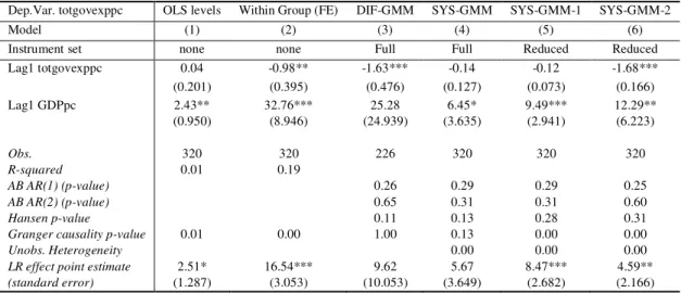
However, there is stronger evidence supporting the reverse relationship, that is, from government expenditures to per capita GDP, therefore favouring the idea of Wagner’s Law. There are significant short and long-run effects, we reject the null of no Granger-causality using our two-step Hansen incremental test, and diagnostics are well behaved (Table 2).
[Table 1-2]
Redoing the OECD sub-sample (not shown), we get slightly stronger results favouring Granger causality from government spending to GDP for a positive short-run effect in 3 out of 6 models. Nevertheless, no significant long-run effect emerges. For the OECD the reverse relationship still holds with evidence of Granger-causality from GDP to government spending, as well as positive and significant short and long-run effects in both the pooled OLS and FE models.
4
Under the null, DRU is asymptotically distributed as r2where r is the number of restrictions. 5
See Bond and Windmeijer (2005). 6
4
3. Concluding remarks
Using a panel data set of 155 developed and developing countries for the period 1970-2010, in a context where government spending and revenue have increased throughout time, we have assessed in which way runs causality and also the possibility of the Wagner Law. We find little evidence of Granger causality from per capita GDP to government expenditure across our econometric specifications. However, there is stronger evidence supporting the reverse relationship, from government expenditures to per capita GDP, therefore favouring the idea of Wagner’s Law. In particular, there are also significant short and long-run effects.
References
1. Arellano, M. (2003), "Panel data econometrics", Oxford University Press, Oxford.
2. Arellano, M. and Bover, O. (1995), "Another Look at the Instrumental Variable Estimation of Error Component Models", Journal of Econometrics, 68: 29-51.
3. Barro, R. J. (1990), ‘Government spending in a simple model of endogenous growth”, Journal of Political Economy, 98, S103-S124.
4. Barro, R. J. (1991), “Economic growth in a cross section of countries”, Quarterly Journal of Economics, 106, 407-44.
5. Bond. S.R. and F. Windmeijer (2005), "Reliable inference for GMM estimates? Finite sample properties of alternative test procedures in linear panel data models", Econometric Reviews, 24(1), 1-37.
6. Devarajan, S. V., V. Swaroop and H. Zou. (1996), “The Composition of Public Expenditure and Economic Growth”, Journal of Monetary Economics, 37, 313-344
7. Grier, K. B. and G. Tullock, (1989) “An Empirical Analysis of Cross-National Economic Growth: 1951-80”, Journal of Monetary Economics, 24(2), 259-76.
8. Hakro, A. N. (2009), “Size of government and growth rate of per capita income in selected Asian Developing countries”, International Research Journal of Finance and Economics, 28.
9. Huang, Y. and Temple, J. (2005), “Does external trade promote financial development?” Bristol Economics Discussion Papers 05/575.
10. Kumar, S. (2009), “Further evidence on public spending and economic growth in East Asian countries”, MPRS WP 19298.
11. Landau, D. (1983), “Government and Economic Growth in the Less Developed Countries: An Empirical Study for 1960-1980”, Economic Development and Cultural Change, 35(1), 35-75.
12. Landau, D. (1983), “Government Expenditure and Economic Growth: A Cross Country Study”, Southern Economic Journal, 49, 783-792.
13. Ram, R. (1986), “Government Size and Economic Growth: A New Framework and Some Evidence from Cross-Section and Time Series Data”, American Economic Review, 76, 191-203.
14. Romer, P. M. (1990), “Endogenous technological change”, Journal of Political Economy, 98, 71-102 15. Sala-i-Martin, X. (1997), “I just ran two million regressions”, American Economic Review, 87, 178-183 16. Yuk, W. (2005), “Government size and economic growth: time series evidence for the UK 19830
5
Table 1: Panel Granger-Causality – GDP per capita and Total Government Expenditures per capita (full sample)
Dep.Var. real GDPpc OLS levels Within Group (FE) DIF-GMM SYS-GMM SYS-GMM-1 SYS-GMM-2
Model (1) (2) (3) (4) (5) (6)
Instrument set none none Full Full Reduced Reduced
Lag1 GDPpc 1.02*** 0.90*** 0.48*** 1.07*** 1.08*** 0.99***
(0.005) (0.044) (0.133) (0.020) (0.028) (0.018)
Lag1 totgovexppc 0.00 -0.00 -0.0002** -0.00 -0.00 -0.00
(0.000) (0.000) (0.000) (0.000) (0.001) (0.000)
Obs. 426 426 320 426 426 426
R-squared 0.99 0.78
AB AR(1) (p-value) 0.37 0.29 0.28 0.40
AB AR(2) (p-value) 0.96 0.02 0.02 0.04
Hansen p-value 0.24 0.20 0.20 0.29
Granger causality p-value 0.95 0.47 0.00 0.00 0.00 0.00
Unobs. Heterogeneity 0.44 0.02 1.00
LR effect point estimate -0.0004 -0.001 -0.0004* 0.001 0.003 -0.01
(standard error) (0.007) (0.0019) (0.0002) (0.002) (0.008) (0.026)
Note: Our five-year averages dataset was used to assess Granger causality. Year dummies are included in all models (coefficients not reported). Figures in parenthesis below point estimates are standard-errors. The GMM results reported here are two-step estimates with heteroskedasticity-consistent standard errors. The Hansen test is used to assess the overidentifying restrictions; the test uses the minimized value of the corresponding two-step GMM estimator. The difference Hansen test is used to test the additional moment conditions used by the system GMM estimators in which SYS GMM uses the standard moment conditions, while SYS GMM-1 only uses the lagged first-differences of GDPpc dated t-2 (and earlier) as instruments in levels and SYS-2 only uses lagged first-differences of totgovexp_gdp dated t-2 (and earlier) as instruments in levels. The heterogeneity test is used to test the null that there are no individual effects (see text). The Granger causality test examines the null hypothesis that GDPpc is not Granger-caused by totgovexp_gdp; the test statistic is criterion based, using restricted and unrestricted models (see main text for details). The LR effect is the point estimate of the long-run effect of totgovexp_gdp on GDPpc. Its standard error is approximated using the delta method. *, **, *** denote significance at 10, 5 and 1% levels.
Table 2: Panel Granger-Causality - Total Government Expenditures per capita and GDP per capita (full sample)
Dep.Var. totgovexppc OLS levels Within Group (FE) DIF-GMM SYS-GMM SYS-GMM-1 SYS-GMM-2
Model (1) (2) (3) (4) (5) (6)
Instrument set none none Full Full Reduced Reduced
Lag1 totgovexppc 0.04 -0.98** -1.63*** -0.14 -0.12 -1.68***
(0.201) (0.395) (0.476) (0.127) (0.073) (0.166)
Lag1 GDPpc 2.43** 32.76*** 25.28 6.45* 9.49*** 12.29**
(0.950) (8.946) (24.939) (3.635) (2.941) (6.223)
Obs. 320 320 226 320 320 320
R-squared 0.01 0.19
AB AR(1) (p-value) 0.26 0.29 0.29 0.25
AB AR(2) (p-value) 0.65 0.31 0.31 0.60
Hansen p-value 0.11 0.13 0.28 0.31
Granger causality p-value 0.01 0.00 1.00 0.13 0.00 0.00
Unobs. Heterogeneity 0.00 0.00 0.00
LR effect point estimate 2.51* 16.54*** 9.62 5.67 8.47*** 4.59**