António Afonso João Tovar Jalles

António Afonso & João Tovar Jalles

T

he

F

iscal

C

onsequences of

D

eflation

: E

vidence from

the

G

olden

A

ge of

G

lobalization

WP23/2016/DE/UECE _________________________________________________________

De pa rtme nt o f Ec o no mic s

W

P

T

HE

F

ISCAL

C

ONSEQUENCES OF

D

EFLATION

:

E

VIDENCE FROM

THE

G

OLDEN

A

GE OF

G

LOBALIZATION

António Afonso

_{João Tovar Jalles}

October 2016

Abstract

We study the fiscal consequences of deflation on a panel of 17 economies in the first wave of globalization, between 1870 and 1914. By means of impulse response analyses and panel regressions, we find that a 1 percent fall in the price level leads to an increase in the public debt ratio of about 0.23-0.32 pp. and accounting for trade openness, monetary policy and the exchange rate raises the absolute value of the coefficient on deflation. Moreover, the public debt ratio increases when deflation is also associated with a period of economic recession. For government revenue, lagged deflation comes out with a statistically significant negative coefficient, while government primary expenditure seems relatively invariant to changes in prices.

JEL: C33, E31, E50, E62

Keywords: debt, deflation, local projection, impulse response functions, GMM, recessions, expansions

* _{We are grateful to Vito Tanzi for very useful comments. The opinions expressed herein are those of the authors and do not}

reflect those of their employers.

$ _{ISEG/UTL - Technical University of Lisbon, Department of Economics; UECE – Research Unit on Complexity and}

Economics. UECE is supported by FCT (Fundação para a Ciência e a Tecnologia, Portugal), email: aafonso@iseg.utl.pt.

# _{Centre for Globalization and Governance, Nova School of Business and Economics, Campus Campolide, Lisbon,}

2 1.Introduction

The economic problems associated with deflation are traditionally linked with sluggish GDP growth

and/or economic recessions. Fisher (1933) first mentioned the idea of debt deflation where falling price

levels would increase outstanding debt values in real terms. This paper contributes to the

understanding of the consequences of deflation for an array of fiscal aggregates, between the end of the

19th _{century and the beginning of the 20}th _{century, just before the start of World War I. Such analysis}

can provide important information for policymakers at any point in time. Firstly, deflation is linked

with mechanical surges in debt-to-GDP ratios as it comprises of pre-existing stocks plus its term

structure, which, together with downward rigidities in sovereign interest rates, tend to additionally

compound the rise of both debt market value and debt ratios. Secondly, deflation also affects the

budget balance by impacting government revenues and primary government expenditures. Current

literature on the consequences of deflation on fiscal aggregates is scarce.1 _{In contrast, several papers}

have looked at the corresponding effects of high inflation2 _{or the reverse direction, i.e., the effect of}

fiscal policy on price dynamics.3 _{Finally, other studies have also analyzed the impact of falling prices}

and its economic costs.4

In the context of our historical timespan we need to be aware that total public spending was only

around 10% of GNP in most countries, while pensions and cash transfers were practically non-existent

and income taxes still did not exist for much of the period under scrutiny, nor did general sales taxes

(see Tanzi and Schuknecht, 2000). Moreover, the gold standard was prevalent and determining

exchange rates and, because of the intensifying industrial revolution, the prices of many products were

falling before the occurrence of any productivity gains.

1 _{Existing studies on deflation have looked more at the role of fiscal policy to boost aggregate demand aiming at exiting}

from a deflationary episode (Auerbach and Obstfeld, 2004; Cochrane, 2011). To our knowledge, End et al. (2015) is the only study that recently took a long-term view on the effects of deflation on fiscal outcomes by supposedly exploring a set of 21 countries between 1850 and 2013 (in reality they only look at 18 countries as enumerated in their footnote 27).

2 _{Olivera (1967) and Tanzi (1977) find that double-digit inflation tends to deteriorate government budget deficits in real}

terms due to lags in tax collections. Aghevli and Kahn (1978) and Heller (1980) further study the links between fiscal policy and inflation in the context of developing economies.

3 _{Catao and Terrones (2005) looked at a panel of 107 countries between 1960 and 2001 and highlighted a robust positive}

relationship between budget deficits and inflation among high-inflation and developing country groups, but not among low-inflation advanced economies. Afonso and Jalles (2016, forthcoming) use SURE estimation methods to assess the link between prices, bond yields and the fiscal behavior. One of their results is that improvements in the fiscal stance lead to persistent falls in sovereign yields and higher sovereign yields are reflected in upward price movements.

4 _{Se notably, DeLong (1999), Furhrer and Tootell (2003), while Svensson (2003) also discusses the intricacies of deflation}

3

In this paper, we empirically assess the impact of deflation and low inflation episodes on several

fiscal aggregates by looking at a sample of 17 countries in the first wave of globalization, that is,

between 1870 and 1914. We also take a positive approach to our empirical question and do not aim to

address the issue related to the optimal fiscal response to deflation. Our main contributions to the

literature are three-fold: i) building a novel dataset for the period at hand; ii) providing short- and

medium-term analyses via the estimation of impulse response functions directly from local projections;

iii) coming up with a long-run assessment of the question at hands via panel estimations.

By means of impulse response analyses and panel regressions our results show that: i) a 1 percent

fall in prices leads to an increase in the debt ratio of about 0.23-0.32 pp accounting for trade openness,

monetary policy and the exchange rate raises the absolute value of the coefficient on deflation.

Moreover, the debt ratio increases when deflation is also associated with an economic recession.

Indeed: ii) for revenues, lagged deflation comes out with a statistically significant negative coefficient,

while government primary expenditure seems relatively invariant to changes in prices; iii) countries

with better institutions do not see their debt ratios rise following a decline in prices while it increases

when deflation is also associated with an economic recession.

The remainder of the paper is organized as follows. Section 2 briefly describes the theoretical

background. Section 3 develops the empirical methodology and section 4 presents the data. Section 5

presents and discusses the main results. The last section concludes.

2. Theoretical Background

Price dynamics affect fiscal policy on several dimensions. Let us begin with public

debt-to-GDP-ratio. For a given country i at time t, we can mathematically represent the governing the dynamics of

the debt-to-GDP ratio, by means of the following equation:5

1

(1

)

t t t t

debt

= +

λ

debt

−

pbal

where

λ

= −

(

r g

)/ (1

+

g

)

growth rate between t-1 and t. Note that

r

=

[(1

+

i

)/ (1

+

π

)] 1

− ⇔ + = +

1

i

(1

r

)(1

+

π

)

i

,

π

corresponding to the nominal interest rate in period t and the change in the GDP deflator between t-1

5 _{Escolano (2010) provide additional information on public deb dynamics, fiscal sustainability and cyclical adjustment of}

4

and t, respectively. In addition,

1

+ = +

γ

(1

g

)(1

+

π

)

γ

between t-1 and t. Hence, Equation (1) is rewritten as:

(2)

It follows from Equation (2) that for any given debt stock and real GDP growth rates, deflation

mechanically increases the debt-to-GDP ratio. Firstly, it lowers nominal GDP, therefore raising the

ratio upwards. Secondly, the primary balance may worsen unexpectedly in an environment marked by

deflation, leading to an additional increase in the debt burden. Thirdly, for any given level of nominal

interest and real GDP growth rates, deflation increases the real value of the overall interest bill. If we

have sticky interest rates or deflation is unanticipated, then nominal rates will not adjust immediately

to absorb the shock. Generally speaking, government interest payments are mostly based on

contractual interest rates, which are essentially fixed and, hence, do not adjust rapidly nor fully in the

short run to fluctuations in domestic prices.6

In addition, deflation can affect primary budget balances through its impact on both government

revenue and expenditure.

On the revenue side, deflation would not affect the revenue-to-GDP ratio if the tax system would

be characterized by full proportionality: the different GDP components would be similarly taxed and

the adjustments in the numerator and denominator would cancel one another. In practical terms,

however, the tax system includes several distortionary features, which means that deflation will in fact

alter revenue-to-GDP ratios (End et al., 2015). Two situations are possible. On the one hand, the

revenue-to-GDP ratio can go down due to the immediate loss of seigniorage revenue (which under a

fiat money system without monetary policy is equivalent to an implicit inflation tax) for any given

level of real money balances, therefore creating a “deflation subsidy”. Moreover, the lack of perfect

indexation mechanisms for movements in the price level, results in a movement of tax payers’

positions between the different tax brackets, which subsequently impact the amount of collected

revenue (Hirao and Aguirre, 1970). In addition, revenue-to-GDP ratios are likely to suffer from

deflation if tax exemptions are widespread, since these are usually expressed in nominal terms. On the

other hand, deflation can facilitate the increase in the revenue-to-GDP ratio if central banks react to

6 _{The impact of this channel is a function of the maturity structure of the sovereign debt as well as its currency}

5

deflationary pressures by means of quantitative easing policies aimed at producing seignorage revenue

(assuming that deflation leads to an increase in real money balances holdings, which expand the

effective taxable base). Furthermore, given that, for example, excises revenues are generally inelastic

to price fluctuations, their fall will in principle push up their ratio with respect to GDP. Lastly, since

prices change faster than wages, consumers reallocate their traditional basket of goods by increasing

the purchases of higher scale products, which are usually more heavily taxed. Similarly, if the GDP

deflator falls quicker than consumption prices, the revenue ratio will increase.7

On the expenditure side, its components tend to be stickier than those of revenues, given the

nominal rigidities embedded in their design and the political difficulties in making cuts to some of

them when prices fall (e.g. public wages or transfers such as pensions and other social benefits). This

means that the only politically feasible solution to deflation episodes is an immediate freeze in nominal

components, leading to a rise in the corresponding ratios-to-GDP. Finally, given that budgets are

normally prepared and executed in nominal terms, it is usually hard to adjust quickly the spending

items to unexpected changes in the fiscal forecasts for a given fiscal year.

3. Empirical Methodology

We follow two main empirical approaches. The first aims to inspect the short and medium-term

effects of deflationary episodes on fiscal aggregates by means of impulse response functions obtained

via the local projection method. The second takes a longer run focus, by estimating a series of panel

regressions.

a) Local Projection Method

To estimate the impact of deflation episodes on fiscal aggregates over the short and medium-term,

we rely on the local projection method popularized by Jorda (2005). For each future period k, the

following regression is estimated on annual data:

(3)

with k=1,…,5 (in years) and where Y represents one of our fiscal dependent variables, namely public

debt, total government revenues, primary expenditure and primary balance (all expressed in percent of

7 _{Lags in tax collections can equally play a role for double-digit deflation rates under cash-basis accounting (Olivera,1967;}

6

GDP); is a dummy variable taking the value 1 at the beginning of a deflationary episode and zero

otherwise8_{, in country i at time t; are country fixed effects; are time effects; and measures}

the impact of for each future period k. In our estimations we set the lag length (l) to two (note,

however, that results are very robust to other lag structures). We use the panel-corrected standard error

(PCSE) estimator by Beck and Katz (1995) to estimate equation (3).

The IRFs are obtained by plotting the resulting estimates for for k= 1,…,5, and the

corresponding confidence interval is computed by means of the standard errors of the estimated

coefficients . Note that, according to Nickell (1981), the inclusion of a lagged dependent variable

and fixed effects can bias the estimation of and in small samples. That said, since the finite

sample bias is equal to 1/45 in our case, this concern is likely to be mitigated. Moreover, robustness

checks to endogeneity confirm the validity of the results.

We are aware of alternative ways of estimating dynamic impacts but, as we will explain, those are

inferior options. The first possible alternative would be to estimate a Panel Vector Autoregression

(PVAR). However, this is generally considered a “back-box” since all relevant regressors are

considered endogenous. Moreover, one has to know the exact order in which they enter in the system.

Since economic theory rarely provides such an ordering, the Choleski decomposition is often used as a

solution of limited value for providing structural information to a VAR. Moreover, a major limitation

of the VAR approach is that it has to be estimated to low order systems. Since all effects of omitted

variables will be in the residuals, this may lead to big distortions in the IRFs, making them of little use

for structural interpretations (see e.g. Hendry 1995). In addition, all measurement errors or

misspecifications will also induce unexplained information left in the error terms, making

interpretations of the IRFs even more difficult (Ericsson et al., 1997). One should bear in mind that due

to its limited number of variables and the aggregate nature of the shocks, a VAR model should be

viewed as an approximation to a larger structural system. In contrast, the approach used here does not

suffer from these identification and size-limitation problems and, in fact, has been suggested by

Auerbach and Gorodnichenko (2013), inter alia, as a sufficiently flexible alternative.

A second alternative of assessing the dynamic impact of fiscal consolidation episodes would be to

estimate an Autoregressive-Distributed-Lag (ARDL) model of changes in markups and compute the

8 _{Taking only the first year of a given deflationary episode improves identification and reduces the scope for possible}

7

IRFs from the estimated coefficients (Romer and Romer, 1989; and Cerra and Saxena, 2008). Note that

the IRFs obtained using this method, however, tend to be lag-sensitive, therefore undermining the

overall stability of the IRFs. Moreover, the statistical significance of long-lasting effects can result

from one-type-of-shock models, particularly when the dependent variable is very persistent (Cai and

Den Haan, 2009). Contrarily, in the local projection method we do not experience such issue since

lagged dependent variables enter as control variables and are not used to derive the IRFs. Lastly,

estimated IRFs’ confidence intervals are computed directly using the standard errors of the estimated

coefficients without the need for Monte Carlo simulations.

In order to explore whether changes in fiscal variables to negative price shocks vary depending on

the phase of the business cycle, the following alternative regression will be estimated:

(4)

with (see Auerbach and Gorodichenko, 2013), where z is an indicator

of the state of the economy (using the real GDP growth rate) normalized to have zero mean and unit

variance. The remainder of the variables and coefficients are defined as in Equation (3). This method is

equivalent to Granger and Teravistra’s (1993) smooth transition autoregressive model and has two

main advantages. First, relative to estimating VARs for each regime it uses a larger number of

observations based on a continuum of states to estimate the IRFs, thus increasing stability and

precision. Secondly, in contrast with a model where each dependent variable is interacted with a proxy

for the business cycle, this method makes it possible to directly test whether the effect of deflation

episodes on fiscal variables varies across different regimes such as expansions and recessions.

b) Panel Data Approach

We estimate the following panel regression:

1 1 1

1 1 2 3 4

0 0 0

it it t i it j it j j it l k it k it

j l k

F

α

δ

γ

α

α

α

α

ε

= = =

∆ = + + + ∆ +

_∑

_∑

_∑

where

F

g

ie

interest rate and

D

8

effects, respectively.

ε

variance.

Equation (5) is initially estimated with panel fixed effects. However, we are aware of the

challenges related to the potential reverse causality between fiscal aggregates and price changes since

budget deficits have a determining role in the formation of the inflation level. Hence, following the

literature, we resort to the Generalized Method of Moment estimation (which takes advantage of the

lagged structure of the data) as a way to address this as well as endogeneity and omitted bias problems.

While good instruments are hard to find, we follow Acemoglu et al. (2013) and Fatas and Mihov

(2013) and make use of lags of the different regressors as well as the constraints on the executive

(retrieved from the Database of Political Institutions) which capture the potential veto points on the

decisions of the government.

4. Data

We focus on a panel of 17 economies (selected based on data availability) in the first wave of

globalization, that is, between 1870 and 1914.9 _{We use the CPI-based inflation rate and real GDP}

growth rate from Bordo and Filardo (2005). When observations are missing, we resort to Warren

Weber’s dataset, that includes information on output and prices for many countries starting in 1810.10

We define deflation as negative inflation and include two measures of low inflation: one corresponding

to inflation rates between 0 and 2 percent (“lowflation 1”) and a second corresponding to inflation rates

between 0 and 1 percent (“lowflation 2”).

As far as fiscal aggregates are concerned, debt ratios come from Abbas et al. (2010) while other

fiscal variables such as government revenues, primary expenditure, interest payments (which allows

the computation of effective interest rates) and primary balance come from Mauro et al. (2013).

Additional controls such as the nominal interest rate (used to compute the interest rate growth

differential), trade openness (exports and imports over GDP), a measure of broad money and the

exchange rate come from Bordo et al. (2001). Political and institutional variables (constraints on the

executive and the polity2 index) come from Polity IV project whose data coverage begins in 1800.

9 _{The country list is: Australia, Belgium, Canada, Denmark, Finland, France, Germany, Italy, Japan, Netherlands, Norway,}

Portugal, Spain, Sweden, Switzerland, UK and US.

9

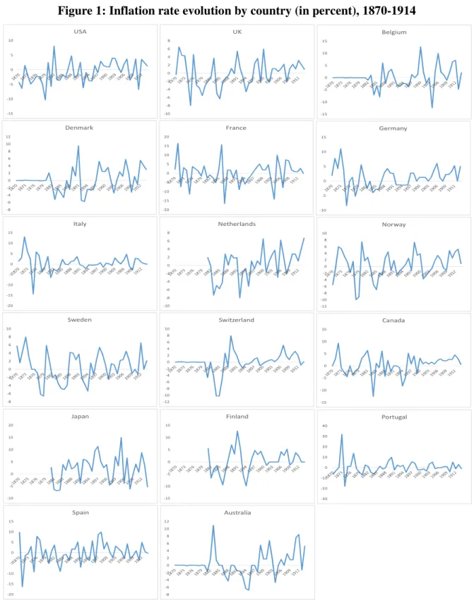
Figure 1: Inflation rate evolution by country (in percent), 1870-1914

-15 -10 -5 0 5 10 USA -10 -8 -6 -4 -2 0 2 4 6 8 UK -15 -10 -5 0 5 10 15 Belgium -8 -6 -4 -2 0 2 4 6 8 10 12 Denmark -20 -15 -10 -5 0 5 10 15 20 France -10 -5 0 5 10 15 Germany -20 -15 -10 -5 0 5 10 15 Italy -10 -8 -6 -4 -2 0 2 4 6 8 Netherlands -12 -10 -8 -6 -4 -2 0 2 4 6 8 10 Norway -8 -6 -4 -2 0 2 4 6 8 10 Sweden -12 -10 -8 -6 -4 -2 0 2 4 6 8 10 Switzerland -15 -10 -5 0 5 10 15 Canada -10 -5 0 5 10 15 20 Japan -15 -10 -5 0 5 10 15 Finland -30 -20 -10 0 10 20 30 40 Portugal -20 -15 -10 -5 0 5 10 15 Spain -8 -6 -4 -2 0 2 4 6 8 10 12 Australia

We begin by plotting, for each country, the time profile of CPI inflation rate to inspect visually the

10

experience, deflation was a relatively common phenomenon in the late 1800s and early 1900s. More

precisely, defining a deflation episode simply as years of negative inflation, Table A1 in the Appendix

shows that our sample between 1870-1914 experienced 297 years combined of deflation,

corresponding to 146 episodes (each lasting an average of about 2 years). Portugal and Spain

experienced the largest number of deflationary episodes (13 in total) over the period under

consideration, while Finland experienced the smallest (four in total).

We further differentiate between deflationary episodes associated with recessions or expansions

in economy activity. Following Borio and Filardo (2004, 2005) we adopt three generic deflation

categories: good deflations, that result from positive supply shocks; bad deflations, that are correlated

with recessions; and ugly deflations, that stand for periods of steep decreases in prices linked with

acute recessions. Without controlling for any other variable, the median debt ratios seem to have gone

up during deflations, particularly if the economy was in a recession. Revenues increase during

deflation and the same is true for primary expenditure. Note, however, that, historical data relate only

to ex-post outturns and include discretionary policy actions put in place in the face of deflation.

Consequently, underlying trends are difficult to identify. The increase in expenditures is higher than

that of revenues, yielding a decline in primary balances with is particularly affected if the economy is

in a slump. In the next section, we discuss the main results of our analysis.

[Table 1]

5. Empirical Results

a. Local Projection Impulse Responses

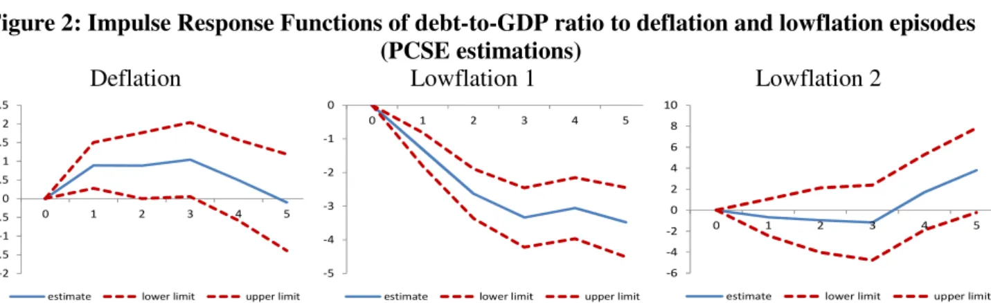
Starting with the debt-to-GDP ratio, the resulting IRFs stemming from estimating the baseline

equation (3) are displayed in Figure 2. The debt ratio rises following a shock in deflation (that is, a

decline in prices) and the effect is statistically significant up to 2 years after the impact (t=0). The

impact of a shock to “lowflation 1” (define as inflation rates between 0 and 2 percent), on the contrary,

leads to a fall in the debt ratio. Using a stricter definition of low inflation, that is, “lowflation 2”, the

effect on the debt ratio is not statistically different from zero, as evidence by the wider confidence

11

Figure 2: Impulse Response Functions of debt-to-GDP ratio to deflation and lowflation episodes (PCSE estimations)

Deflation

-2 -1.5 -1 -0.5 0 0.5 1 1.5 2 2.5

0 1 2 3 4 5

estimate lower limit upper limit

Lowflation 1

-5 -4 -3 -2 -1 0

0 1 2 3 4 5

estimate lower limit upper limit

Lowflation 2

-6 -4 -2 0 2 4 6 8 10

0 1 2 3 4 5

estimate lower limit upper limit

Note: Dotted lines equal one standard error confidence bands. Seem main text for details.

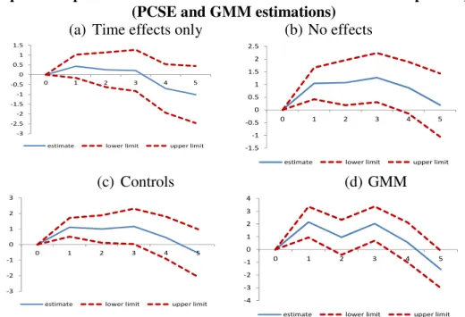
In order to check the robustness of the previous set of results, Equation (3) is re-estimated for

the case of deflation11 _{by including only time effects to control for specific time shocks, as those}

affecting world interest rates. The results for this specification are shown in Figure 3 panel (a).

Moreover, as shown by Tuelings and Zubanov (2010), a possible bias from estimating Equation (3)

using country-fixed effects is that the error term of the equation may have a non-zero expected value,

due to the interaction of fixed effects and country-specific price developments. This would lead to a

bias of the estimates that is a function of k. To address this issue and further check the robustness of

our findings, Equation (3) was re-estimated by excluding both country and time fixed effects from the

analysis. The results reported in Figure 3 panel (b) suggest that this bias is negligible (the difference in

the point estimate is small and not statistically significant).

Estimates of the impact of deflation on the debt ratio could be biased because of endogeneity,

as unobserved factors influencing the dynamics of prices may also affect the probability of the

occurrence of a deflation episode. Therefore, Equation (3) was augmented to control for the real GDP

growth rate and the effective interest rate. The results of this exercise are reported in Figure 3 panel (c)

and confirm the robustness of the previous findings.

In addition, in order to deal with endogeneity concerns we re-estimate Equation (3) by means

of a GMM estimator (Arellano and Bover, 1995). This estimator is particularly relevant when series

are very persistent and the lagged levels may be weak instruments in the first differences. In this case,

lagged values of the first differences can be used as valid instruments in the equation in levels and

12

efficiency is increased by running Equation (3) by means of a system GMM estimator.12 _{Results in}

Figure 3 panel (d) are qualitatively in line with our previous findings.

Figure 3: Impulse Response Functions of debt-to-GDP ratio to deflation episodes, robustness (PCSE and GMM estimations)

(a) Time effects only

-3 -2.5 -2 -1.5 -1 -0.5 0 0.5 1 1.5

0 1 2 3 4 5

estimate lower limit upper limit

(b) No effects

-1.5 -1 -0.5 0 0.5 1 1.5 2 2.5

0 1 2 3 4 5

estimate lower limit upper limit

(c) Controls -3 -2 -1 0 1 2 3

0 1 2 3 4 5

estimate lower limit upper limit

(d) GMM -4 -3 -2 -1 0 1 2 3 4

0 1 2 3 4 5

estimate lower limit upper limit

Note: Dotted lines equal one standard error confidence bands. Seem main text for details. In panel c) controls include real

GDP growth rate and the effective interest rate.

As an additional sensitivity check, Equation (3) was re-estimated for different lags (l) of

changes in the dependent variable. The results (not shown for reasons of parsimony but are available

upon request) confirm that previous findings are not sensitive to the choice of the number of lags.

In Figure 4 we replace the debt ratio by other fiscal variables. A decrease in the general price

level leads to an immediate rise in revenues and a medium term decline in primary expenditures,

resulting in an improvement of the primary balance. Given that the deflation impact on the debt ratio is

positive, this effect can only be explained (in face of Equation 2) by the positive effect to a decline in

prices stemming from the interest rate-growth differential (as we observe in panel d).

12 _{The list of instruments includes the first and second lags of all the right-hand-side variables as well as constraints on the}

13

Figure 4: Impulse Response Functions of other fiscal aggregates to deflation episodes (PCSE estimations) (a) Revenue -0.15 -0.1 -0.05 0 0.05 0.1 0.15 0.2 0.25 0.3 0.35

0 1 2 3 4 5

estimate lower limit upper limit

(b) Primary expenditure

-0.4 -0.3 -0.2 -0.1 0 0.1 0.2

0 1 2 3 4 5

estimate lower limit upper limit

(c) Primary balance

0 0.05 0.1 0.15 0.2 0.25 0.3 0.35 0.4 0.45

0 1 2 3 4 5

estimate lower limit upper limit

(d) Interest rate-growth differential

0 0.5 1 1.5 2 2.5 3 3.5 4

0 1 2 3 4 5

estimate lower limit upper limit

Note: Dotted lines equal one standard error confidence bands. Seem main text for details.

Figure 5: Impulse Response Functions to deflation episodes, contingent on the phase of the business cycle (PCSE estimations)

Debt -1 -0.5 0 0.5 1

0 1 2 3 4 5

estimate_booms lower limit upper limit estimate_busts lower limit upper limit

Revenue -0.15 -0.1 -0.05 0 0.05 0.1

0 1 2 3 4 5

estimate_booms lower limit upper limit estimate_busts lower limit upper limit

Primary expenditure -0.15 -0.1 -0.05 0 0.05 0.1

0 1 2 3 4 5

estimate_booms lower limit upper limit estimate_busts lower limit upper limit

Primary balance -0.1 -0.05 0 0.05 0.1 0.15

estimate_booms lower limit

upper limit estimate_busts

lower limit upper limit

14

To explore whether the deflationary effect on fiscal variables varies depending on the phase of

the business cycle, we estimate Equation (4) for debt, revenues, primary expenditures and primary

balances. Results in Figure 5, suggest that the rise in the debt ratio is statistically significant higher in

bad times; in good times despite deflation, debt actually falls. Revenues (primary expenditures) rise

(fall) following a deflation shock if the economy is booming, leading to an improvement in the budget

position.

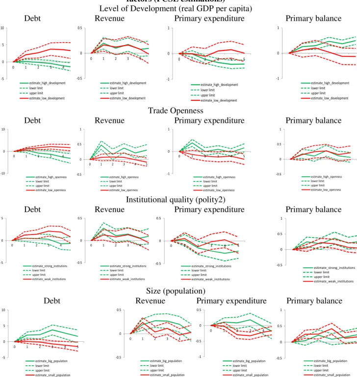
In order to control for additional relevant country features, we now assess whether the effect of

deflation episodes on fiscal aggregates depends on countries’ structural and policy variables: the level

of economic development (real GDP per capita), country size (population), trade openness (exports

plus imports over GDP) and institutional quality (polity2).

Highly distorted trade policies especially policies that create a heavy bias against exports

increase a country’s indebtedness. Borrowing to finance public expenditures partly account for the big

rise in growth of external debt (Paesani, Strauch and Kremer, 2006).

The more frequently coalitions or ruling parties change, the higher the propensity of a

government to accumulate debt (Alesina et al. 1993; Poterba, 1994; Hallerberg and Strauch, 2002).

Countries characterized by a short average tenure of government have a tendency to expand debt

(Roubini and Sachs, 1989).

It is also important to control for country size, since higher automatic stabilizers reduce fiscal

multipliers and the larger economies tend to be able to have higher automatic responses to the business

cycle (Batini et al., 2014). In addition, economies with lower propensity to import have higher fiscal

multipliers because of fewer demand leakage via imports (Barrell et al., 2012).

To this end, Equation (3) is re-estimated using structural/policy variables’ 2nd _{quartile as the}

threshold value to split the whole sample into two sub-samples that will be compared against the

15

Figure 6: Impulse Response Functions to deflation episodes, the role of structural and policy factors (PCSE estimations)

Level of Development (real GDP per capita)

Debt Revenue Primary expenditure Primary balance

-5 0 5 10

0 1 2 3 4

estimate_high_development lower limit upper limit estimate_low_development -0.5 0 0.5

0 1 2 3 4

estimate_high_development lower limit upper limit estimate_low_development -1 0 1

0 1 2 3 4 5

estimate_high_development lower limit upper limit estimate_low_development -1 0 1 estimate_high_development lower limit upper limit estimate_low_development Trade Openness

Debt Revenue Primary expenditure Primary balance

-10 0 10

0 1 2 3 4

estimate_high_openness lower limit upper limit estimate_low_openness -0.5 0 0.5 1

0 1 2 3 4 5

estimate_high_openness lower limit upper limit estimate_low_openness -1 0 1

0 1 2 3 4 5

estimate_high_openness lower limit upper limit estimate_low_openness -0.5 0 0.5 1 estimate_high_openness lower limit upper limit estimate_low_openness Institutional quality (polity2)

Debt Revenue Primary expenditure Primary balance

-5 0 5

0 1 2 3 4

estimate_strong_institutions lower limit upper limit estimate_weak_institutions -0.5 0 0.5

0 1 2 3 4

estimate_strong_institutions lower limit upper limit estimate_weak_institutions -0.5 0 0.5

0 1 2 3 4 5

estimate_strong_institutions lower limit upper limit estimate_weak_institutions -0.5 0 0.5 1 estimate_strong_institutions lower limit upper limit estimate_weak_institutions Size (population)

Debt Revenue Primary expenditure Primary balance

-5 0 5 10

0 1 2 3 4 5

estimate_big_population lower limit upper limit estimate_small_population -0.5 0 0.5

0 1 2 3 4 5

estimate_big_population lower limit upper limit estimate_small_population -1 -0.5 0 0.5

0 1 2 3 4

estimate_big_population lower limit upper limit estimate_small_population -0.5 0 0.5 1 estimate_big_population lower limit upper limit estimate_small_population

16

Looking at Figure 6, first row, countries with a lower development level experience a higher

impact of debt to a fall in general prices. The difference in the effects of falling prices on revenue

between high and low real GDP per capita levels is not statistically significant from one another.

More (less) open economies experience a decline (rise) in the debt ratio following a negative

shock in prices. Revenue ratios also behave favourably the more open an economy is (the effect is not

statistically different from zero from relatively closed economies).

Countries with better institutions (proxying for better checks and balances, political

competition, less corruption, etc.) do not see their debt ratios rise following a decline in prices.

Countries with weak institutions however, do get higher debt ratios as a reaction to deflation.

Democracy and political accountability seem to work towards increased efforts in cutting primary

expenditures ratios in the medium term following price declines, an effect that is less mitigated in the

case of worse institutional settings.

Finally, the larger the country the bigger the rise in debt ratios after a negative shock to prices.

Moreover, revenues (primary expenditures) rise (fall) more following a deflation shock in larger

(smaller) countries.

b. Panel Analysis

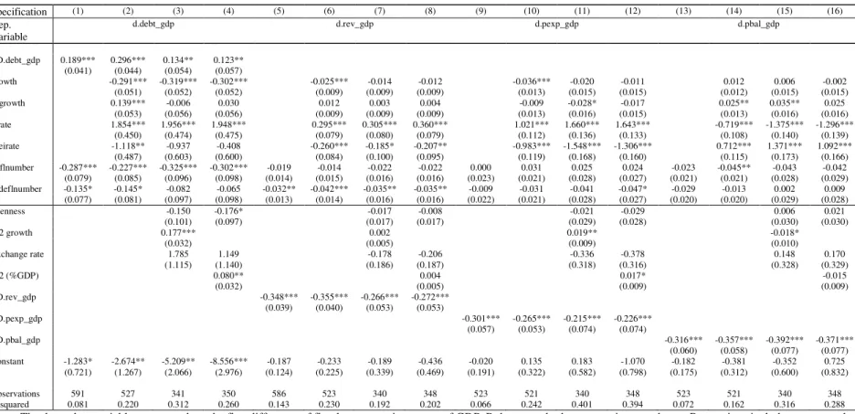
The results of the baseline regression on the impact of negative inflation on debt ratios are

displayed in Table 2, column 1. We see that a 1 percent fall in prices leads to an increase in the debt

ratio of about 0.29 pp. There is some persistence as indicated by the lagged regressor (magnitude of

around 0.16 pp). In column 2 we add some controls and observe that higher GDP growth lowers the

debt ratio, but a rise in the effective interest rate increases it. Both effects are in line with the

theoretical predications. The effect of 1 percent deflation corresponds now to an increase in the debt

ratio of about 0.30-0.32 pp accounting for trade openness, monetary policy and the exchange rate

raises the absolute value of the coefficient on deflation. Turning to revenues, the contemporaneous

effect of deflation does not seem to have a statistically significant impact regardless of the set of

controls included. Its lag, however, yields a statistically significant negative coefficient. This means

that a fall of 1 percent in the price level leads to a rise in the revenue to GDP ratio of about 0.03-0.04

pp, a rather marginally small effect. This could be seen as a reverse Olivera-Tanzi effect, when high

17

relatively invariant to changes in prices. Both these effects combined, lead to a positive impact of

deflation of primary balance, in the order of 0.05 pp for a 1 percent decline in the inflation rate.

[Table 2]

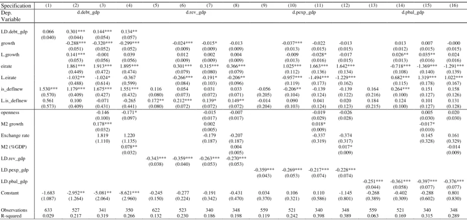
In Table 3 we repeat the same exercise, but now instead of the actual negative inflation values,

we replace our main regressor by a dummy variable taking the value 1 when the inflation rate is

negative and zero otherwise. This exercise is easily comparable to the analysis of the IRFs done in

section 5.a), and looking at the debt ratio, and yields similar results as before, since the deflation

dummy has a positive and statistically significant impact in all four specifications. The remaining

regressors retain the previous signs and significance. Yet again, for revenues only the lagged dummy

variable yields a statistically significant positive coefficient and the same for specification 14 for the

primary balance.

[Table 3]

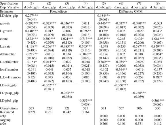
Next, we take the specification equivalent to (2), (6), (10) and (14), respectively for debt,

revenues, primary expenditures and primary balance and include both deflation and our first measure

of low inflation together.13 _{A 1 percent decline in prices leads to a 0.22 pp increase in debt ratio and a}

0.05 pp increase in primary balance (see Table 4). Estimation by difference GMM is qualitatively

unchanged for the case of primary balance and while the deflation impact on contemporaneous debt

disappears, the lagged effect is considerably larger in absolute terms. Note that the null of Hansen

J-test for over-identifying restrictions is not rejected, meaning that the model specification is correct and

all over-identified instruments are exogenous. The tests for serial correlation also point to the absence

of second-order serial correlation in the residuals

[Table 4]

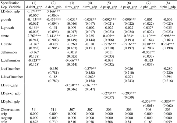
In Table 5 we redo the analysis but estimating by difference GMM specifications where

deflation and our measure “lowflation1” are included separately. The contemporaneous impact of

deflation increases the primary balance while low inflation seems to affect only revenues. The lag

13 _{Results with “lowflation2” do not qualitatively change the main conclusions and are available from the authors upon}

18

deflation coefficient however, is statistically significant in the cases of debt and revenue ratios. A 1

percent decline in prices leads to a 0.32 pp and 0.07 pp increase in debt and revenue ratios,

respectively.

[Table 5]

In Table 6 we include the interaction between our deflation variables (either negative inflation rate

or the dummy variable) and positive/negative real GDP growth rates. The debt ratio seems to increase

when deflation is also associated with an economic recession.14

Looking at panel b), we also observe that revenue ratios fall in reaction to a price decline

shock particularly during bad times. Primary expenditures, on the contrary, seem to decrease when

deflation is associated with growth in real GDP.

[Table 6]

We now move away from fiscal ratios to inspecting the impact of deflation on nominal fiscal

levels. In fact, the analysis of fiscal variables expressed in percent of GDP points to the fact that the

denominator effect is more important for the results, and some of the impact of deflation on the

numerator (the nominal fiscal variable) may therefore be muted. Following End et al. (2015), we build

“pseudo-nominal” changes in the fiscal variable x=X/Y by means of the following formula for our

specific panel setup:

1

[(1 )(1 ) 1] x it

a it it it it it

it

X

x x g

Y₋ π

∆

∆ = = ∆ + + + − . (6)

The change corrected from the denominator effect, ∆axit, proxies the nominal increase, as measured

in terms of previous year GDP, where

π

the real GDP growth rate. Re-estimating equation (3) with the newly created “pseudo-nominal”

changes gives us the results displayed in Table 7. As before, nominal debt rises to falling prices and the

14 _{The link between deflation and recessions are also highlighted notably by Atkeson and Kehoe (2004) and Bordo and}

19

same is true for both nominal revenues and nominal primary expenditures. Results are consistent

between panels a) and b), that is, whether we use fixed effects or difference GMM estimations.

[Table 7]

Finally, we check if our previous results are robust to the use of episodes of deflation (defined as

years of negative inflation), instead of annual observations of negative inflation rate or a dummy

variable approach. More specifically, we take the 146 deflation episodes in a cross-section regression

where all the relevant regressors are averaged over the corresponding episode period. We display in

Table 8 the results from this OLS regression. In this case, deflation episodes contribute to increase

government spending ratios but contribute to decrease both the debt ratio and the primary balance

ratios.

[Table 8]

6. Conclusion

Lessons from the past, notably from the fiscal consequences of deflation in the Golden Age of

Globalization, are relevant in terms of current and recent fiscal and price developments in several

economies. Therefore, in this paper we have used a panel of 17 economies, in the the decades before

World War I, between 1870 and 1914, to study the fiscal consequences of deflation.

Our results show that a 1 percent fall in prices leads to an increase in the debt ratio of about

0.23-0.32 pp accounting for trade openness, monetary policy and the exchange rate raises the absolute value

of the coefficient on deflation. Moreover, the debt ratio increases when deflation is also associated

with an economic recession. For government revenue, lagged deflation comes out with a statistically

significant negative coefficient, while government primary expenditure seems relatively invariant to

changes in prices. Interestingly, countries with better institutions do not see their debt ratios rise

following a decline in prices. On the other hand, the debt ratio increases when deflation is also

associated with an economic recession. In addition, estimations by difference GMM are qualitatively

unchanged vis-à-vis the baseline results.

Even though we are able to find relevant results and some insightful policy indications, one has to

bear in mind that changes in fiscal aggregates are not purged from discretionary actions reacting to

deflation, and also that today’s economies have undergone through a series of structural reforms that

20

between our analysis period and current times, given both the smaller size of the government, and also

the rather different environment and typical household characteristics in, for instance, 1870. 15

References

1. Abbas, A., N. Belhocine, A. El Ganainy, and M. Horton, (2011), “Historical Patterns and Dynamics of Public Debt—Evidence from a New Database,” IMF Economic Review, 59(4), 717–42

2. Afonso, A. and Jalles, J. T. (2016, forthcoming), “The Price Relevance of Fiscal Developments”, International Economic Journal.

3. Aghevli, B. B. and M. S. Khan, (1978), “Government Deficits and the Inflationary Process in Developing Countries,” IMF Staff Papers, 25(3), 383–416.

4. Akitoby, B., T. Komatsuzaki, and A. Binder, (2014), “Inflation and Public Debt Reversals in the G7 Countries,” IMF Working Paper No. 14/96 (Washington: International Monetary Fund).

5. Arellano, M. and Bover, O. (1995), "Another Look at the Instrumental Variable Estimation of Error Component Models", Journal of Econometrics, 68, 29-51.

6. Auerbach, A. J. and M. Obstfeld, (2004), “Monetary and Fiscal Remedies for Deflation,” NBER Working Paper No. 10290 (Cambridge, Massachusetts: National Bureau of Economic Research).

7. Auerbach, A. and C. Gorodnichenko, 2013, “Measuring the Output Responses to Fiscal Policy.” American Economic Journal: Economic Policy 4 (2), 1–27.

8. Barrell, R., Holland, D., Hurst, I. (2012). “Fiscal Consolidation: Part 2. Fiscal Multipliers and Fiscal Consolidations,” OECD Economics Department Working Paper No. 933 (Paris: Organisation for Economic Co-operation and Development).

9. Batini, N., Eyraud, L., Forni, L., Weber, A. (2014). “Fiscal Multipliers: Size, Determinants, and Use in Macroeconomic Projections”, IMF Technical Notes and Manuals No. 2014/4.

10. Beck, N. L., and J. N. Katz, (1995), “What to do (and not to do) with time-series cross-section data”, American Political Science Review, 89, 634–647.

11. Beckworth, D., (2008), “Aggregate Supply-Driven Deflation and Its Implications for Macroeconomic Stability,” Cato Journal, 28(3), 363–384.

12. Bernanke, B., (2002), “Deflation: Making Sure It Doesn’t Happen Here,” Speech before the National Economist Club.

13. Bordo, M. and A. Filardo, (2005), “Deflation and Monetary Policy in a Historical Perspective: Remembering the Past or Being Condemned to Repeat It?,” Economic Policy, 20(44), 799–844.

21

14. Bordo, M., Eichengreen, B., Klingebiel, D., Martinex-Peria, M. S. (2001), “Is the Crisis problem growing more severe?”, Economic Policy, 16 (32).

15. Borio, C. and A. Filardo, (2004), “Looking Back at the International Deflation Record,” The North American Journal of Economics and Finance, 15(3), 287–311.

16. Cai, X., and W. J. Den Haan (2009), “Predicting Recoveries and the Importance of Using Enough Information”, CEPR Discussion Paper No. 7508.

17. Catao, L. A.V. and M. E. Terrones, (2005), “Fiscal Deficits and Inflation,” Journal of Monetary Economics, 52, 529–554.

18. Cerra, V., and S. Saxena, (2008), “Growth Dynamics: The Myth of Economic Recovery,” American Economic Review, 98(1), 439-57.

19. Cochrane J. H., (2011), “Understanding Policy in the Great Recession: Some Unpleasant Fiscal Arithmetic,” European Economic Review, 55(1), 2–30.

20. DeLong, B., (1999), “Should We Fear Deflation?” Brookings Papers on Economic Activity, 1, 225–52.

21. End, N. Tapsoba, S., Terrier, G., Duplay, R. (2015), “Deflation and Public Finances: Evidence from the Historical Records”, IMF Working Paper 15/176.

22. Ericsson, N. R., Hendry, D. F., and Mizon, G. E., 1997. Exogeneity, cointegration and economic policy analysis. Journal of Business and Economic Statistics, 16, 370–387.

23. Escolano, J. (2010), “A practical guide to public debt dynamics, fiscal sustainability and cyclical adjustment of budgetary aggregates”, IMF Technical Notes and Manuals, FAD, Washington DC.

24. Fisher, I., (1933), “The Debt-Deflation Theory of Great Depression,” Econometrica, 1(4), 337– 357.

25. Fuhrer, J. and G. Tootell (2003), “Issues in Economics: What Is the Cost of Deflation?” Regional Review, Q3, 2–5.

26. Gordon, R. (2016). The Rise and Fall of American Growth: The U.S. Standard of Living since the Civil War, Princeton University Press.

27. Granger, C. W. J., Newbold, P. (1974), “Spurious regressions in econometrics”, Journal of Econometrics 2, 111-120.

28. Heller, P. S., (1980), “Impact of Inflation on Fiscal Policy in Developing Countries,” IMF Staff Papers, 27(4).

29. Hendry, D.F., 1995, Dynamic Econometrics. New York, Oxford University Press.

30. Hirao, T, and Aguirre, C. (1978), “Maintaining the Level of Income Tax Collections under Inflationary Conditions”, IMF Staff Papers, 17 (2), 277-325.

22

32. Mauro, P., R. Romeu, A. J. Binder, and A. Zaman, (2013), “A Modern History of Fiscal Prudence and Profligacy,” IMF Working Paper No. 13/5 (Washington: International Monetary Fund).

33. Nickell, S. (1981), “Biases in dynamic models with fixed effects”, Econometrica, 49, 1417– 1426

34. Olivera, J. G. H., (1967), “Money, Prices and Fiscal Lags: A Note on the Dynamics of Inflation,” Quarterly Review della Banca Nazionale del Lavoro, 20, 258–267.

35. Romer, C., and D. Romer (1989), “Does Monetary Policy Matter? A New Test in the Spirit of Friedman and Schwartz,” NBER Macroeconomics Annual, 4, 121–70.

36. Svensson, L., (2003), “Escaping from a Liquidity Trap and Deflation: The Foolproof Way and Others,” Journal of Economic Perspectives, 17(4), 145–66.

37. Tanzi, V., (1977), “Inflation, Lags in Collection, and the Real Value of Tax Revenue,” IMF Staff Papers, 24,154–67 (Washington: International Monetary Fund).

38. Tanzi. V. and Schuknecht, L. (2000). Public Spending in the 20th _{Century: A Global}

Perspective, Cambridge: Cambridge University Press.

23

Table 1: Summary Statistics of Changes in Debt, Revenue, Primary Expenditure and Primary Balance

overall Deflation and growth

Deflation and recession

overall Deflation and growth

Deflation and recession

ΔDebt (% GDP) Min -12.45 -38.83 -1.95 ΔRevenue (%

GDP)

Min -4.99 -4.99 -2.61 Q1 -0.74 -1.25 -0.04 Q1 -0.20 -0.25 -0.20 Median 0.53 -0.29 1.66 Median 0.07 0.01 0.12 Q3 2.69 1.75 3.38 Q3 0.34 0.34 0.82 Max 9.89 11.16 20.12 Max 3.63 3.20 3.63

overall Deflation and growth

Deflation and recession

overall Deflation and growth

Deflation and recession ΔPrimary

expenditure (% GDP)

Min -3.53 -3.53 -2.64 ΔPrimary balance (%GDP)

Min -13.22 -13.22 -3.66

Q1 -0.23 -0.33 -0.05 Q1 -0.24 -0.23 -0.49 Median 0.07 0.03 0.15 Median -0.02 -0.02 -0.07 Q3 0.34 0.34 0.55 Q3 0.26 0.35 0.19 Max 14.78 14.78 3.58 Max 3.11 3.11 1.47

Note: Δ denotes the change in the fiscal aggregate. Min, Q1, Median, Q3, Max, denote the minimum, first quartile, median, third quartile, and maximum

Table 2: Baseline regression on the fiscal impact of deflation value - fixed effects

Specification (1) (2) (3) (4) (5) (6) (7) (8) (9) (10) (11) (12) (13) (14) (15) (16)

Dep. Variable

d.debt_gdp d.rev_gdp d.pexp_gdp d.pbal_gdp

LD.debt_gdp 0.189*** 0.296*** 0.134** 0.123** (0.041) (0.044) (0.054) (0.057)

growth -0.291*** -0.319*** -0.302*** -0.025*** -0.014 -0.012 -0.036*** -0.020 -0.011 0.012 0.006 -0.002

(0.051) (0.052) (0.052) (0.009) (0.009) (0.009) (0.013) (0.015) (0.015) (0.012) (0.015) (0.015)

L.growth 0.139*** -0.006 0.030 0.012 0.003 0.004 -0.009 -0.028* -0.017 0.025** 0.035** 0.025

(0.053) (0.056) (0.056) (0.009) (0.009) (0.009) (0.013) (0.016) (0.015) (0.013) (0.016) (0.016)

eirate 1.854*** 1.956*** 1.948*** 0.295*** 0.305*** 0.360*** 1.021*** 1.660*** 1.643*** -0.719*** -1.375*** -1.296***

(0.450) (0.474) (0.475) (0.079) (0.080) (0.079) (0.112) (0.136) (0.133) (0.108) (0.140) (0.139)

L.eirate -1.118** -0.937 -0.408 -0.260*** -0.185* -0.207** -0.983*** -1.548*** -1.306*** 0.712*** 1.371*** 1.092***

(0.487) (0.603) (0.600) (0.084) (0.100) (0.095) (0.119) (0.168) (0.160) (0.115) (0.173) (0.166)

deflnumber -0.287*** -0.227*** -0.325*** -0.302*** -0.019 -0.014 -0.022 -0.022 0.000 0.031 0.025 0.024 -0.023 -0.045** -0.043 -0.042

(0.079) (0.085) (0.096) (0.098) (0.014) (0.015) (0.016) (0.016) (0.023) (0.021) (0.028) (0.027) (0.021) (0.021) (0.028) (0.029)

L.deflnumber -0.135* -0.145* -0.082 -0.065 -0.032** -0.042*** -0.035** -0.035** -0.009 -0.031 -0.041 -0.047* -0.029 -0.013 0.002 0.009

(0.077) (0.081) (0.097) (0.098) (0.013) (0.014) (0.016) (0.016) (0.022) (0.021) (0.028) (0.027) (0.020) (0.020) (0.029) (0.028)

openness -0.150 -0.176* -0.017 -0.008 -0.021 -0.029 0.006 0.021

(0.101) (0.097) (0.017) (0.017) (0.029) (0.028) (0.030) (0.030)

M2 growth 0.177*** 0.002 0.019** -0.018*

(0.032) (0.005) (0.009) (0.010)

Exchange rate 1.785 1.149 -0.178 -0.206 -0.336 -0.378 0.148 0.170

(1.115) (1.140) (0.186) (0.187) (0.318) (0.316) (0.328) (0.329)

M2 (%GDP) 0.080** 0.004 0.017* -0.015

(0.032) (0.005) (0.009) (0.009)

LD.rev_gdp -0.348*** -0.355*** -0.266*** -0.272***

(0.039) (0.040) (0.053) (0.053)

LD.pexp_gdp -0.301*** -0.265*** -0.215*** -0.226***

(0.057) (0.053) (0.074) (0.074)

LD.pbal_gdp -0.316*** -0.357*** -0.392*** -0.371***

(0.060) (0.058) (0.077) (0.077)

Constant -1.283* -2.674** -5.209** -8.556*** -0.187 -0.233 -0.189 -0.436 -0.020 0.135 0.183 -1.070 -0.182 -0.381 -0.352 0.725

(0.721) (1.267) (2.066) (2.976) (0.124) (0.225) (0.339) (0.469) (0.191) (0.322) (0.582) (0.798) (0.175) (0.312) (0.600) (0.832)

Observations 591 527 341 350 586 523 340 348 523 521 340 348 523 521 340 348

R-squared 0.081 0.220 0.312 0.260 0.143 0.230 0.192 0.202 0.066 0.242 0.401 0.394 0.072 0.162 0.316 0.288

Table 3: Baseline regression on the fiscal impact of deflation dummy - fixed effects

Specification (1) (2) (3) (4) (5) (6) (7) (8) (9) (10) (11) (12) (13) (14) (15) (16)

Dep. Variable

d.debt_gdp d.rev_gdp d.pexp_gdp d.pbal_gdp

LD.debt_gdp 0.066 0.301*** 0.144*** 0.134** (0.040) (0.044) (0.054) (0.057)

growth -0.288*** -0.320*** -0.299*** -0.024*** -0.015* -0.013 -0.037*** -0.022 -0.013 0.013 0.007 -0.000

(0.051) (0.052) (0.052) (0.009) (0.009) (0.009) (0.013) (0.015) (0.015) (0.012) (0.015) (0.015)

L.growth 0.141*** -0.001 0.039 0.012 0.002 0.004 -0.009 -0.028* -0.017 0.026** 0.035** 0.024

(0.053) (0.056) (0.056) (0.009) (0.009) (0.009) (0.013) (0.016) (0.015) (0.013) (0.016) (0.016)

eirate 1.861*** 1.913*** 1.895*** 0.301*** 0.315*** 0.366*** 1.025*** 1.663*** 1.642*** -0.718*** -1.369*** -1.291***

(0.449) (0.472) (0.474) (0.079) (0.080) (0.079) (0.112) (0.136) (0.134) (0.108) (0.140) (0.139)

L.eirate -1.032** -1.024* -0.367 -0.266*** -0.191* -0.206** -0.957*** -1.494*** -1.229*** 0.682*** 1.319*** 1.022***

(0.488) (0.614) (0.599) (0.084) (0.103) (0.096) (0.119) (0.173) (0.162) (0.115) (0.178) (0.167)

is_deflnew 1.530*** 1.179*** 1.675*** 1.551*** 0.116 0.054 0.031 0.033 -0.056 -0.206** -0.139 -0.139 0.164 0.264*** 0.151 0.158

(0.570) (0.409) (0.427) (0.432) (0.080) (0.073) (0.072) (0.071) (0.205) (0.104) (0.124) (0.122) (0.216) (0.100) (0.127) (0.126)

L.is_deflnew 0.561 0.100 -0.071 -0.265 0.172** 0.212*** 0.139* 0.149** -0.014 0.090 0.041 0.020 0.184 0.124 0.101 0.131

(0.573) (0.409) (0.431) (0.441) (0.080) (0.072) (0.072) (0.072) (0.204) (0.103) (0.124) (0.123) (0.215) (0.100) (0.127) (0.128)

openness -0.146 -0.171* -0.015 -0.007 -0.019 -0.026 0.005 0.020

(0.100) (0.097) (0.017) (0.017) (0.029) (0.028) (0.030) (0.030)

M2 growth 0.178*** 0.002 0.018* -0.017*

(0.032) (0.005) (0.009) (0.010)

Exchange rate 1.819 1.220 -0.179 -0.207 -0.337 -0.374 0.145 0.161

(1.110) (1.135) (0.187) (0.187) (0.319) (0.317) (0.328) (0.329)

M2 (%GDP) 0.078** 0.004 0.017* -0.014

(0.032) (0.005) (0.009) (0.009)

LD.rev_gdp -0.343*** -0.359*** -0.263*** -0.270***

(0.038) (0.040) (0.053) (0.053)

LD.pexp_gdp -0.359*** -0.269*** -0.217*** -0.228***

(0.043) (0.053) (0.074) (0.074)

LD.pbal_gdp -0.251*** -0.361*** -0.397*** -0.376***

(0.044) (0.058) (0.077) (0.077)

Constant -1.683 -2.952** -5.081** -8.621*** -0.245 -0.277 -0.191 -0.431 0.034 0.106 0.110 -1.145 -0.268 -0.402 -0.288 0.801

(1.087) (1.264) (2.064) (2.960) (0.150) (0.224) (0.342) (0.470) (0.370) (0.321) (0.586) (0.801) (0.389) (0.309) (0.602) (0.830)

Observations 633 527 341 350 622 523 340 348 559 521 340 348 559 521 340 348

R-squared 0.029 0.217 0.319 0.266 0.132 0.230 0.186 0.198 0.119 0.242 0.398 0.389 0.063 0.169 0.315 0.289

Table 4: Regression on the fiscal impact of deflation and lowflation value included together – fixed effects and difference GMM

Specification (1) (2) (3) (4) (5) (6) (7) (8) Dep. Variable d.debt_gdp d.rev_gdp d.pexp_gdp d.pbal_gdp d.debt_gdp d.rev_gdp d.pexp_gdp d.pbal_gdp Estimator Fixed effects Difference GMM

LD.debt_gdp 0.297*** 0.184*** (0.044) (0.061)

growth -0.293*** -0.025*** -0.036*** 0.011 -0.446*** -0.037** -0.090*** -0.003 (0.051) (0.009) (0.013) (0.012) (0.094) (0.017) (0.022) (0.023) L.growth 0.140*** 0.012 -0.009 0.026** 0.179* 0.002 -0.029 0.043* (0.053) (0.009) (0.014) (0.013) (0.100) (0.018) (0.024) (0.023) eirate 1.872*** 0.300*** 1.021*** -0.713*** 2.933*** 0.245 0.402* -1.081***

(0.452) (0.079) (0.113) (0.109) (0.956) (0.151) (0.206) (0.167) L.eirate -1.138** -0.266*** -0.983*** 0.705*** -1.348 -0.253 -0.587*** 0.829***

(0.490) (0.084) (0.119) (0.116) (0.982) (0.165) (0.211) (0.202) deflnumber -0.219** -0.013 0.034 -0.046** -0.176 0.002 0.018 -0.064* (0.088) (0.016) (0.022) (0.022) (0.142) (0.027) (0.037) (0.035) L.deflnumber -0.151* -0.044*** -0.029 -0.018 -0.380*** -0.055** -0.026 -0.035 (0.084) (0.015) (0.021) (0.021) (0.137) (0.026) (0.033) (0.034) lowf1number -0.161 -0.041 -0.037 -0.018 -0.102 -0.364** -0.019 -0.137 (0.407) (0.073) (0.104) (0.100) (0.856) (0.166) (0.227) (0.232) L.lowf1number 0.128 0.045 -0.030 0.085 1.082 -0.178 -0.258 0.387* (0.402) (0.072) (0.103) (0.100) (0.849) (0.160) (0.252) (0.222) LD.rev_gdp -0.352*** -0.350***

(0.041) (0.047)

LD.pexp_gdp -0.264*** -0.288*** (0.054) (0.059)

LD.pbal_gdp -0.357*** -0.366*** (0.058) (0.062) Observations 527 523 521 521 511 507 506 506 R-squared 0.221 0.231 0.242 0.164

ar1p 0.000 0.000 0.000 0.000 sarganp 0.000 0.000 0.000 0.000 ar2p 0.766 0.140 0.531 0.112

27

Table 5: Regression on the fiscal impact of deflation and lowflation value included separately – difference GMM

Specification (1) (2) (3) (4) (5) (6) (7) (8) Dep. Variable d.debt_gdp d.debt_gdp d.rev_gdp d.rev_gdp d.pexp_gdp d.pexp_gdp d.pbal_gdp d.pbal_gdp LD.debt_gdp 0.174*** 0.166***

(0.060) (0.060)

growth -0.443*** -0.456*** -0.031* -0.038** -0.092*** -0.090*** 0.005 -0.009 (0.092) (0.094) (0.016) (0.017) (0.021) (0.022) (0.022) (0.023) L.growth 0.164* 0.151 0.009 -0.002 -0.022 -0.027 0.037* 0.035

(0.098) (0.096) (0.017) (0.017) (0.023) (0.024) (0.022) (0.023) eirate 2.769*** 3.143*** 0.263* 0.225 0.405** 0.363* -1.110*** -0.998***

(0.941) (0.909) (0.149) (0.144) (0.206) (0.193) (0.164) (0.161) L.eirate -1.167 -0.425 -0.260 -0.101 -0.576*** -0.516*** 0.830*** 0.924***

(0.965) (0.905) (0.163) (0.151) (0.210) (0.197) (0.200) (0.190) deflnumber -0.167 -0.019 0.011 -0.065**

(0.128) (0.025) (0.033) (0.033) L.deflnumber -0.323** -0.066*** -0.033 -0.023 (0.128) (0.024) (0.032) (0.033)

lowf1number -0.630 -0.379** 0.026 -0.280 (0.781) (0.158) (0.210) (0.220) L.lowf1number 0.188 -0.262* -0.274 0.294

(0.789) (0.154) (0.243) (0.216) LD.rev_gdp -0.350*** -0.361***

(0.046) (0.047)

LD.pexp_gdp -0.273*** -0.293*** (0.057) (0.059)

LD.pbal_gdp -0.359*** -0.380*** (0.061) (0.062) Observations 511 511 507 507 506 506 506 506 ar1p 0.000 0.000 0.000 0.000 0.000 0.000 0.000 0.000 sarganp 0.000 0.000 0.000 0.000 0.000 0.000 0.000 0.000 ar2p 0.878 0.730 0.510 0.058 0.508 0.541 0.163 0.059

28

Table 6: Regression on the fiscal impact of deflation during economic expansions and recessions - difference GMM

Specification (1) (2) (3) (4) (5) (6) (7) (8) Dep. Variable d.debt_gdp d.debt_gdp d.rev_gdp d.rev_gdp d.pexp_gdp d.pexp_gdp d.pbal_gdp d.pbal_gdp a) Inflation number

defgrowthnumber -0.694 -0.012 -0.035 -0.034 (0.559) (0.034) (0.049) (0.047) L.defgrowthnumber 0.765 -0.057* -0.040 -0.033 (0.517) (0.031) (0.041) (0.045)

defrecessionnumber -0.234 0.089 0.125 0.093 (0.173) (0.103) (0.128) (0.142) L.defrecessionnumber -0.464*** -0.016 0.068 0.061

(0.159) (0.109) (0.144) (0.147) b)Inflation dummies

deflgrowth 2.003 0.199 -0.869** 0.391 (1.755) (0.200) (0.422) (0.241) L.deflgrowth -1.646 0.559*** -0.807* 0.561** (1.804) (0.191) (0.465) (0.245)

deflrecession 1.292 -0.865** 0.164 0.061 (1.046) (0.386) (0.243) (0.441) L.deflrecession 2.580*** -0.074 0.160 0.352

(0.949) (0.378) (0.240) (0.465) Note: The dependent variable corresponds to the first difference of fiscal aggregate in percent of GDP. Robust standard errors are in parentheses. Regressions include country and time effects omitted for reasons of parsimony. *,**,*** denote statistical significant at the 10, 5 and 1 percent levels, respectively.

Table 7: Regression on the fiscal impact of deflation and low inflation in nominal terms (adjusted variables) – fixed effects and difference GMM

Specification (1) (2) (3) (4) (5) (6) (7) (8) Dep. Variable d.debt_adj d.debt_adj d.rev_adj d.rev_adj d.pexp_adj d.pexp_adj d.pbal_adj d.pbal_adj

a) Fixed effects

deflnumber 0.696*** 0.101*** 0.123*** -0.021 (0.093) (0.015) (0.022) (0.021) L.deflnumber -0.538*** -0.008 -0.007 -0.008 (0.094) (0.016) (0.022) (0.020)

lowf1number -0.214 -0.030 0.025 -0.063 (0.463) (0.074) (0.104) (0.097) L.lowf1number 0.277 0.057 -0.008 0.069

(0.457) (0.074) (0.104) (0.097) b) Difference GMM

deflnumber 0.953*** 0.122*** 0.150*** -0.028 (0.164) (0.029) (0.035) (0.036) L.deflnumber -0.263 -0.025 -0.002 0.010

(0.181) (0.031) (0.036) (0.037)

lowf1number 0.541 -0.117 0.387 -0.199 (1.059) (0.199) (0.261) (0.233) L.lowf1number 1.561 0.099 0.108 0.340

(0.242)

29

Table 8: Baseline regression on the fiscal impact of deflation episodes – cross-section

Specification (1) (2) (3) (4) Dep. Variable debt_gdp rev pexp pbal

growth -0.371*** -0.024 -0.041** 0.021 (0.086) (0.017) (0.020) (0.020) eirate 0.478* 0.091* 0.017 0.068

(0.248) (0.050) (0.059) (0.061) deflnumber -0.182* 0.009 0.056** -0.043* (0.096) (0.019) (0.022) (0.023) Constant -0.814 -0.131 0.249 -0.354 (0.997) (0.201) (0.238) (0.243) Observations 108 107 105 104 R-squared 0.208 0.056 0.099 0.052

30 Appendix