António Afonso João Tovar Jalles The Price Relevance of Fiscal Developments

(1)

António Afonso & João Tovar Jalles

The Price Relevance of Fiscal Developments

WP16/2015/DE/UECE _________________________________________________________ De pa rtme nt o f Ec o no mic s

W

ORKING

P

APERS

(2)

The Price Relevance of Fiscal Developments

*

November 2015

António Afonso

$

and João Tovar Jalles



Abstract

We use SURE estimation methods to assess the link between prices, bond yields and the fiscal behavior. A first equation determines the country-specific cost of government financing via the long-term government bond yield, as a function of budget balance positions. A second equation links the price level to the cost of government financing. Our results for 15 EU countries in the period 1980Q1-2013Q4, show that: improvements in the fiscal stance lead to persistent falls in sovereign yields; higher sovereign yields are reflected in upward price movements; improvements in the fiscal stance in recession times lead to short-term decreases in yields; better fiscal stance in expansions induce downward movement in bond yields only after 8 quarters.

JEL: E31, E62, H62, O52

Keywords: price level, yields, Ricardian regimes, SURE, local projection, impulse response function

*_{The opinions expressed herein are those of the authors and do not necessarily reflect those of their employers. Any remaining errors} are the authors’ sole responsibility.

$_{ISEG/UL - University of Lisbon, Department of Economics; UECE}_–_{Research Unit on Complexity and Economics. UECE is}

supported by FCT (Fundação para a Ciência e a Tecnologia, Portugal), email: aafonso@iseg.utl.pt.

_{Centre for Globalization and Governance, Nova School of Business and Economics, Campus Campolide, Lisbon, 1099-032}

(3)

2

1. INTRODUCTION

The relevance of fiscal developments for price behaviour and inflation can be traced back to some recent theoretical work linked to the so-called Fiscal Theory of the Price Level (FTPL), initially made popular by Leeper (1991), Sims (1994) and Woodford (1994, 1995). On the other hand, this discussion links further back to Sargent and Wallace (1975), and to the controversy of using rules to control the nominal interest rate, which may lead to price level indeterminacy.1 In this case, Leeper-Sims-Woodford (hereafter LSW) argue that it will be then up to the government budget constraint to play a key role in the determination of the price level. In other words, fiscal policy may have a relevant role in determining the price level, and then inflation would not be

“always and everywhere a monetary phenomenon”.

Nevertheless, several authors argued against such theoretical possibility, notably McCallum (1999, 2001), McCallum and Nelson (2005), and Buiter (2002). In addition, most available empirical assessments, provided by, for instance, Canzoneri, and Diba (1996), Canzoneri, Cumby and Diba ( 2001a,b), Cochrane (1998) and Woodford (1995), and Afonso (2008), point to the lack of adherence to the idea that the price level may be determined via the intertemporal government budget constraint, given that governments turn out to be rather Ricardian. In other words, primary government budget balances react to government debt to ensure fiscal solvency, and money and prices are determined by money supply and demand, implying the existence of an active monetary policy, and a passive fiscal policy. Still, Rother (2004) reports that activist fiscal policy may have relevant effects on inflation volatility.

This paper adds to the literature by applying Seemingly Unrelated Regressions (SURE) estimation methods to a set of two core specifications linking prices, sovereign bond yields and fiscal developments. The first equation determines the country-specific cost of government financing via the long-term government bond yield, as a function of budget balance positions, and other relevant determinants. The second equation links the price level to its determinants, notably the cost of government financing and the business cycle.

1

In this context, we can mention a “weak form” of the FTPL, due to Sargent and Wallace (1981), where fiscal policy is exogenous, and impinges on the price level via the money supply (see, Carlstrom, and Fuerst, 2000); and a “strong

(4)

3 Our main results show that: i) improvements in the fiscal stance lead to persistent falls in sovereign yields; ii) higher sovereign yields are reflected in upward price movements; iii) improvements in the fiscal stance in recession times lead to short-term decreases in yields, followed by a correction after 10 quarters; iv) better fiscal stance in expansion times induce downward movement in bond yields only after 8 quarters.

The remainder of the paper is organized as follows. Section 2 briefly presents the theoretical framework. Section 3 presents the data and the econometric methodology. Section 4 discusses the empirical results and the last section concludes.

2. THEORETICAL FRAMEWORK

The idea of non-Ricardian regimes rests on the hypothesis that primary budget balances could be determined by the government without taking into account the level of government debt. In that vision of the world, money and prices would then need to adjust to the level of government debt to guarantee the fulfilment of the government intertemporal budget constraint, a passive monetary policy.

Therefore, in the context of a non-Ricardian regime, the fiscal authority may autonomously decide on the budget balance and government debt, influencing the determination of the price level, while the monetary authority would set endogenously the money supply and take the price level from the government budget constraint. In practice we would see an influence of fiscal developments on the price level, either indirectly via the effects of the sovereign bond long-term interest rate on inflation, or via the fiscal effects on the sovereign bond yield and the yield itself.

According to LSW in a non-Ricardian regime, the government budget constraint determines a unique price level (P):

₁ 0(1 )

t j t

j j

t

s B

P r

 

 







(1)

where, Bt – nominal government liabilities (including debt and money base); st – real primary government budget surplus (with seigniorage revenue); r– real interest rate, constant by hypothesis, and with the usual transversality condition (no-Ponzi game condition)

lim ₁ 0 (1 )

t j j

B

j r

  

(5)

4 In a non-Ricardian regime, (1) is fulfilled if after the government has chosen a sequence for primary balances, the price level adjusts endogenously. If (1) is fulfilled for any price level, then it will be fiscal policy to adjust implying a Ricardian regime. Therefore, this discussion can have relevant policy implications given notably the empirical possibility that fiscal developments do impinge on the price level and on inflation.

3. DATA AND ECONOMETRIC METHODOLOGY

3.1Static Approach: estimating a panel data system of equations

We employ Seemingly Unrelated Regressions estimation methods with an iteration procedure over the estimated disturbance covariance matrix and parameter estimates that converge to stable Maximum Likelihood (ML) results (see Zellner, 1962, 1963; and Zellner and Huang, 1962 for further details). The following system with two equations is estimated:

1 1 1 1 1

0 1

it i t it it it

ltbond     capb  stockret  (3)

2 2 2 2 2

0 1

it i t it it it

p    ltbond  gap  . (4)

The first equation determines the country-specific cost of government financing ltbondit, defined as the country’s long-term bond yield, as a function of structural budget balance positions, that is, the cyclically adjusted primary balance,capbit, and the stock market index,stockretit. The second

equation defines the price level, p_it, as a function of the country-specific cost of government financing, ltbondit, and controls for the business cycle by including the output gap, gapit.

On the one hand, we want to check whether a direct effect on inflation of the borrowing costs of the government is present, via equation (4). On the other hand, we also expect that those borrowing costs tend to be higher the higher are the fiscal imbalances, an effect that is specified via equation (3). Therefore, in this SURE framework, it is possible to test for both direct and indirect effects of fiscal developments on the price level.

(6)

5 In order to estimate the impact of fiscal developments (long term bond yield) on long term bonds yield (prices) over the short and medium run, we follow the method proposed by Jorda (2005), which consists of estimating impulse response functions (IRFs) directly from local projections. For each period k the following equation is estimated on quarterly data:

𝑌𝑖,𝑡+𝑘− 𝑌𝑖,𝑡 = 𝛼𝑖𝑘+ 𝑇𝑖𝑚𝑒𝑡𝑘+ ∑𝑗=1𝑙 𝛾𝑗𝑘∆𝑌𝑖,𝑡−𝑗+ 𝛽𝑘𝑋𝑖,𝑡+ 𝜀𝑖,𝑡𝑘 (5)

with k=1,…,12 (in quarters) and where Y represents one of our dependent variables as indicated in Equations (3) and (4), long-term bond yields and the price level, respectively; 𝑋_𝑖,𝑡 denotes either the CAPB or long term bond yield, depending on the equation under scrutiny, in country i at time t; 𝛼_𝑖𝑘 are country fixed effects; 𝑇𝑖𝑚𝑒_𝑡𝑘 is a time trend; and 𝛽_𝑘 measures the impact of 𝑋_𝑖,𝑡 for each future period k. Since fixed effects are included in the regression the dynamic impact should be interpreted as compared to a baseline country-specific trend. In the main results, the lag length (l) is set at 2, even if the results are extremely robust to different numbers of lags included in the specification (see robustness checks and sensitivity presented in the next section). Equation (5) is estimated using the panel-corrected standard error (PCSE) estimator (Beck and Katz, 1995).

Impulse response functions are obtained by plotting the estimated 𝛽_𝑘 for k= 1,…,12, with confidence bands computed using the standard deviations of the estimated coefficients 𝛽_𝑘. While the presence of a lagged dependent variable and country fixed effects may in principle bias the estimation of 𝛾_𝑗𝑘 and 𝛽_𝑘in small samples (Nickell, 1981), the length of the time dimension mitigates this concern.2_{The robustness checks for endogeneity confirm the validity of the results.}

An alternative way of estimating, for instance, the dynamic impact of fiscal developments is to estimate an ARDL equation and to compute the IRFs from the estimated coefficients (Romer and Romer, 1989; and Cerra and Saxena, 2008). However, the IRFs derived using this approach tend to be sensitive to the choice of the number of lags this making the IRFs potentially unstable. In addition, the significance of long-lasting effects with ARDL models can be simply driven by the use of one-type-of-shock models (Cai and Den Haan, 2009). This is particularly true when the dependent variable is highly persistent, as in our analysis. In contrast, the approach used here does not suffer from these problems because the coefficients associated with the lags of the change in the dependent variable enter only as control variables and are not used to derive the IRFs, and since the

2

(7)

6 structure of the equation does not impose permanent effects. Finally, confidence bands associated with the estimated IRFs are easily computed using the standard deviations of the estimated coefficients and Montecarlo simulations are not required.

4. EMPIRICAL ANALYSIS

For the empirical analysis we have considered 15 European Union countries (Austria, Belgium, Estonia, Finland, France, Germany, Greece, Ireland, Italy, Netherlands, Portugal, Slovenia, Slovak Republic, Spain and the UK) throughout the period 1980Q1-2013Q4.3_{We get our data from the}

Eurostat via Datastream.

4.1.Panel Unit Roots

Prior to presenting and discussing our main empirical results, one concern when working with time-series data is the possibility of spurious correlation between the variables of interest (Granger and Newbold, 1974). This situation arises when series are not stationary.4_{Given the notoriously low}

power of individual country-by-country tests for unit roots and cointegration, it is preferable to pool the time series of interest and conduct panel analysis. We employ three different types of panel unit root tests: two first generation tests, namely the Im et al. (2003) test (IPS); the Maddala and Wu (1999) test (MW) and one second generation test – the Pesaran (2007) CIPS test. The latter is associated with the fact that previous tests do not account for cross-sectional dependence of the contemporaneous error terms and failure to consider it may cause substantial size distortions in panel unit root tests (Pesaran, 2007). Tables A1 and A2 in the Appendix show the results and reveal that the unit root null hypothesis can be generally rejected (with the exception of public debt, which

– when mentioned – will be used in first differences).

4.2.Baseline Results

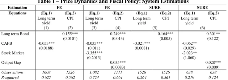
In Table 1 we report the baseline results for the price and yield specifications. We observe that an improvement in the government’s fiscal balance (corrected by the cycle) leads to a fall in long-term bond yields, therefore signaling a credible fiscal strategy and path and less concerns

3

Sample selection was dictated by data availability.

4

(8)

7 about long-term sustainability. Moreover, higher bond yields are triggered by inflationary pressures and larger output gaps. Highly positive output gaps are traditionally associated with over-heating and significant price rises. Our results are robust to single equation estimation (via fixed effects) and system of equations estimation (SURE).5_{In addition, the short and medium-term impacts of the}

budget balance on long term bonds are shown in Figure 1 for the baseline regression without controls and for one where the stock market index and the output gap are added as regressors. Each figure shows the estimated impulse response function and the associated one standard error bands (dotted lines), where the horizontal axis measures quarters.

Table 1 – Price Dynamics and Fiscal Policy: System Estimations

Estimation FE FE SURE SURE

Equations (Eq.1) (Eq.2) (Eq.1) (Eq.2) (Eq.1) (Eq.2) (Eq.1) (Eq.2)

Long term yield

CPI Long term yield

CPI

(1) (2) (3) (4) (5) (6)

Long term Bond 0.155*** 0.249*** 0.164*** 0.301**

(0.0101) (0.013) (0.005) (0.122)

CAPB -0.053*** -0.035*** -0.021*** -0.062**

(0.0188) (0.011) (0.0081) (0.029)

Stock Market -3.355*** -2.023**

(0.2013) (1.060)

Output Gap 0.035*** 0.028***

(0.0083) (0.009)

Observations 1608 1526 1,082 1111 1526 1526 638 638

R-squared 0.627 0.562 0.724 0.661 0.264 0.361 0.219 0.124

Note: Estimation by panel fixed effects (FE) with robust standard errors and seemingly unrelated regression (SURE). The former includes two equations estimated separately; the latter includes one system of two equations estimated jointly. Standard errors are in parenthesis. Constant term was omitted for reasons of parsimony. Fixed effects regressions include time effects omitted for reasons of parsimony. *, **, *** denote significance at 10, 5 and 1% levels.

In general, an improvement in the fiscal stance leads to a persistent fall in the yield of sovereign bonds. Long-term sovereign bond yields fall by about 2-3 bp in the short term (after 3 quarters) and by nearly 6bp in the medium term (after 12 quarters). This is consistent with results notably from Heppke-Falk and Hüfner (2004), Manganelli and Wolswijk (2009), and by Afonso and Guimarães (2014). On the other hand, higher sovereign yields are also reflected in upward price movements.6

5

The use of alternative estimators, such as 2SLS or 3SLS (not shown but available upon request), yielded qualitatively similar results.

6

(9)

8

Figure 1. Baseline Impulse Response Functions

a) Impact of CAPB on long-term bond yields b) Impact of long-term bond yields on CPI

Note: Dotted lines equal one standard error confidence bands. See main text for more details.

In order to check the robustness of the results, Equation (5) is re-estimated by including time fixed effects to control for specific time shocks, as those affecting world interest rates. The results for this specification remain statistically significant and broadly unchanged (Figure 2 panel (a)).

Moreover, as shown by Tuelings and Zubanov (2010), a possible bias from estimating Equation (5) using country-fixed effects is that the error term of the equation may have a non-zero expected value, due to the interaction of fixed effects and country-specific fiscal developments. This would lead to a bias of the estimates that is a function of k. to address this issue and check the robustness of our findings, Equation (5) was re-estimated by excluding country fixed effects from the analysis. The results reported in Figure 2 panel (b) suggest that this bias is negligible (the difference in the point estimate is small and not statistically significant).

Estimates of the impact of fiscal developments on long term bond yields could be biased because of endogeneity, as unobserved factors influencing the dynamics of public finances may also affect the probability of the occurrence of a consolidation episode. In particular, a significant deterioration in economic activity, which would affect unemployment, may determine an increase in the public debt ratio via the budgetary effect of the automatic stabilizers, and therefore increase the probability of consolidation. To address this issue, Equation (5) was augmented to control for the output gap and stock market developments. The results of this exercise are reported in Figure 2 panel (c) and confirm the robustness of the previous findings.

-0.08 -0.07 -0.06 -0.05 -0.04 -0.03 -0.02 -0.01 0 0.01

0 1 2 3 4 5 6 7 8 9 10 11 12

estimate lower limit upper limit

-0.1 0 0.1 0.2 0.3 0.4 0.5

0 1 2 3 4 5 6 7 8 9 10 11 12

(10)

9

Figure 2. Sensitivity and Robustness of Impulse Response Functions

Impact of CAPB on long-term bond yields Impact of long-term bond yields on CPI a) Including country and time effects

b) No country effects

c) Controlling for stock market and output gap

As an additional sensitivity check, Equation (5) was re-estimated for different lags (l) of changes in the Gini coefficient. The results confirm that previous findings are not sensitive to the choice of the number of lags (results are not shown for reasons of parsimony but are available upon request). In addition, in order to deal with endogeneity concerns we re-estimate Equation (5) by means of a GMM estimator (Arellano and Bover, 1995). This estimator is particularly relevant when series are very persistent and the lagged levels may be weak instruments in the first

-0.1 -0.08 -0.06 -0.04 -0.02 0 0.02

0 1 2 3 4 5 6 7 8 9 10 11 12

0 0.1 0.2 0.3 0.4 0.5 0.6 0.7

0 1 2 3 4 5 6 7 8 9 10 11 12 estimate lower limit upper limit

-0.07 -0.06 -0.05 -0.04 -0.03 -0.02 -0.01 0 0.01

0 1 2 3 4 5 6 7 8 9 10 11 12

-0.05 0 0.05 0.1 0.15 0.2 0.25 0.3 0.35 0.4 0.45

0 1 2 3 4 5 6 7 8 9 10 11 12

-0.12 -0.1 -0.08 -0.06 -0.04 -0.02 0 0.02 0.04

0 1 2 3 4 5 6 7 8 9 10 11 12

0 0.05 0.1 0.15 0.2 0.25 0.3

0 1 2 3 4 5 6 7 8 9 10 11 12

(11)

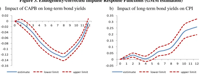
10 differences. In this case, lagged values of the first differences can be used as valid instruments in the equation in levels and efficiency is increased by running Equation (5) by means of a system GMM estimator.7_{Results in Figure 3 are qualitatively in line with our previous findings.}

Figure 3. Endogeneity-corrected Impulse Response Functions (GMM estimation)

a) Impact of CAPB on long-term bond yields b) Impact of long-term bond yields on CPI

To explore whether long term bond yields vary depending on the phase of the business cycle, the following alternative regression will be estimated:

𝑌𝑖,𝑡+𝑘− 𝑌𝑖,𝑡 = 𝛼𝑖𝑘+ 𝑇𝑖𝑚𝑒𝑡𝑘+ ∑𝑙𝑗=1𝛾𝑗𝑘∆𝑌𝑖,𝑡−𝑗+ 𝛽𝑘𝑟𝑒𝑐∙ 𝑌(𝑧) ∙ 𝑋𝑖,𝑡 + 𝛽𝑘𝑒𝑥𝑝∙ (1 − 𝑌(𝑧)) ∙ 𝑋𝑖,𝑡+ 𝜀𝑖,𝑡𝑘 (6)

with 𝑌(𝑧_𝑖𝑡) = exp (−𝛾𝑧𝑖𝑡)

1+exp (−𝛾𝑧𝑖𝑡), 𝛾 > 0

where z is an indicator of the state of the economy (using the output gap computed by means of the HP filter with a smoothing parameter of 1600 applied to real GDP) normalized to have zero mean and unit variance.8 The remainder of the variables and coefficients are defined as in Equation (5).

7

The list of instruments includes the first and second lags of all the right-hand-side variables. The null of Hansen J-test for over-identifying restrictions is not rejected, meaning that the model specification is correct and all over-identified instruments are exogenous. The tests for serial correlation also point to the absence of second-order serial correlation in the residuals.

8

This approach is equivalent to the smooth transition autoregressive (STAR) model developed by Granger and Teravistra (1993). The main advantage of this approach relative to estimating structural VARs for each regime is that it considers a larger number of observations to compute the impulse response functions, thus making the responses more stable and precise.

-0.16 -0.14 -0.12 -0.1 -0.08 -0.06 -0.04 -0.02 0 0.02

0 1 2 3 4 5 6 7 8 9 10 11 12

-0.05 0 0.05 0.1 0.15 0.2 0.25 0.3 0.35

0 1 2 3 4 5 6 7 8 9 10 11 12

(12)

11

Figure 4. State-contingent Impulse Response Functions: Recessions vs. Expansions a) Impact of cyclically adjusted primary balance-to-GDP ratio on long-term bond yields

Recession Expansion

b) Impact of long term bonds on CPI

Recession Expansion

Results presented in Figure 4 panel (a) seem to suggest that improvements in the fiscal stance that took place in times of economic recessions led to a short-term decrease in long-term bond yields, followed by a correction after 9 quarters. On the other hand, in expansions, the overall impact in both the short and medium-term is not statistically different from zero. In panel (b) there seems to exist little difference in the impact of long term bonds on prices between recessions and expansions in the short run, but not in the medium run. During booms the positive impact of long-term bond yields on the price level is higher, relative to times of economic slack.

4.3.Robustness: Structural and Policy Variables

In order to control for additional relevant country features, we now assess whether the effect of fiscal behaviour on long-term bond yields and the effect of these on the price level depend on

countries’ structural and policy variables: the level of economic development (real GDP per capita), country size (population), indebtedness (debt-to-GDP ratio), and trade openness (exports plus

-0.2 -0.15 -0.1 -0.05 0 0.05 0.1

0 1 2 3 4 5 6 7 8 9 10 11 12

-0.2 -0.15 -0.1 -0.05 0 0.05 0.1

0 1 2 3 4 5 6 7 8 9 10 11 12

0 0.1 0.2 0.3 0.4 0.5 0.6 0.7 0.8 0.9

0 1 2 3 4 5 6 7 8 9 10 11 12

0 0.1 0.2 0.3 0.4 0.5 0.6 0.7 0.8 0.9

0 1 2 3 4 5 6 7 8 9 10 11 12

(13)

12 imports over GDP). To test whether the factors mentioned above affect the response of long-term bond yields to impulses on the CAPB and the response of CPI to impulses on long term bonds yields, Equation (5) is re-estimated using structural/policy variables’ 2nd quartile as the threshold value to split the whole sample into two sub-samples that will be compared against the baseline.

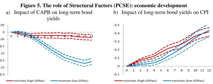
Figure 5. The role of Structural Factors (PCSE): economic development

a) Impact of CAPB on long-term bond yields

b) Impact of long-term bond yields on CPI

Note: Lines represent the impulse responses of long term bond yields to a CAPB shock (panel a)) or the impulse response of CPI to a long-term bond yield shock (panel b)). Blue (red) line represents the impulse response of those countries below (above) the corresponding threshold. The dotted lines denote the corresponding confidence bands. The threshold point for each structural (or policy) factor considered corresponds to the 2nd_quartile

(above/below). See main text for more details. Horizontal axis indicates years after the shock.

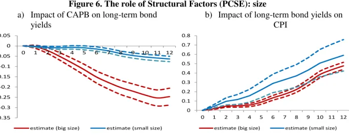
Starting with Figure 5 one observes that the lower the level of development, the higher the negative response of long-term bond yields to an improvement in the overall fiscal position. This can be linked to the fact that per capita GDP is usually a relevant determinant of sovereign ratings and low income countries might be seen by capital markets as more fiscally vulnerable to changes in the fiscal stance. 9 Moreover, the positive impact of long-term bond yields on the price level is higher in countries with smaller real GDP per capita, at least in the short run. Also, bigger countries experience a more sizeable negative response of long-term bond yields to a shock in the CAPB, relative to smaller countries (Figure 6), which can imply that for smaller economies, long-term yields are rather more exogenously determined. The positive spillover of high bond yields into higher prices is also higher in countries with less population, at least in the short run (the confidence bands cross one another around 7 quarters).

9

See, for instance, Afonso et al., (2012). -0.3

-0.25 -0.2 -0.15 -0.1 -0.05 0 0.05

0 1 2 3 4 5 6 7 8 9 10 11 12

estimate (high GDPpc) estimate (low GDPpc)

-0.1 0 0.1 0.2 0.3 0.4 0.5

0 1 2 3 4 5 6 7 8 9 10 11 12

(14)

13

Figure 6. The role of Structural Factors (PCSE): size

Note: vide footnote figure 5. Mutatis mutandis.

Figure 7. The role of Policy Factors (PCSE): debt level

Turning to policy factors, countries with higher debt-to-GDP ratios tend to experience a sharper downward response of bond yields to an improvement in the fiscal position, compared to countries with lower debt (Figure 7). Hence, for more indebted economies, capital markets may perceive a higher gain in terms of future correction of fiscal imbalances, allowing the long-term yields to decrease as a premium to a so-called Ricardian behavior from the fiscal authority.

On the contrary, in countries with higher debt levels, an increase in bond yields does not translate into much higher prices, relative to countries with lower public indebtedness positions. Finally, trade openness also seems to play a role. The more open the country, the smaller (larger) response of bond yields (prices) to a shock in CAPB (bond yields) in the medium(short) run-Figure 8.

-0.35 -0.3 -0.25 -0.2 -0.15 -0.1 -0.05 0 0.05

0 1 2 3 4 5 6 7 8 9 10 11 12

estimate (big size) estimate (small size)

0 0.1 0.2 0.3 0.4 0.5 0.6 0.7 0.8

0 1 2 3 4 5 6 7 8 9 10 11 12 estimate (big size) estimate (small size)

-0.25 -0.2 -0.15 -0.1 -0.05 0

0 1 2 3 4 5 6 7 8 9 10 11 12

estimate (high debt) estimate (low debt) 0 0.1 0.2 0.3 0.4 0.5 0.6 0.7 0.8 0.9

(15)

14

Figure 8. The role of Policy Factors (PCSE): trade openness

5. CONCLUSION

We have assessed the link between prices, sovereign bond yields and fiscal behavior for a set of 15 EU countries in the period 1980Q1-2013Q4. Our analysis strategy checked whether there is a direct effect on inflation of the borrowing costs of the government, via a first specification, and we then also study the effect of fiscal imbalances on the borrowing costs themselves, via a second equation, therefore, using estimation in a SURE framework.

In order to account for the possibility of non-stationarity in the panel, we have resorted to second generation unit root tests to account for cross-sectional dependence of the contemporaneous error terms. In fact, with the exception of public debt, which was used in first differences, the presence of unit roots was rejected.

Our main results show that: improvements in the fiscal stance lead to persistent falls in sovereign bond yields; higher sovereign yields are reflected in increasing price levels; improvements in the fiscal stance, modelled with the cyclically adjusted primary balance, in recession times lead to short-term decreases in sovereign bond yields; and improvements in the fiscal stance in economic expansions induce downward movements in sovereign bond yields only after 8 quarters.

In terms of robustness, we have also concluded, notably, that the lower the level of development, the higher the negative response of long-term bond yields to an improvement in the fiscal position. Moreover, the positive impact of long-term bond yields on the price level is higher

-0.2 -0.18 -0.16 -0.14 -0.12 -0.1 -0.08 -0.06 -0.04 -0.02 0 0.02

0 1 2 3 4 5 6 7 8 9 10 11 12

estimate (high openness) estimate (small openness)

-0.1 0 0.1 0.2 0.3 0.4 0.5 0.6 0.7

0 1 2 3 4 5 6 7 8 9 10 11 12

(16)

15 in countries with smaller real GDP per capita, at least in the short run. Also, bigger countries experience a more sizeable negative response of long-term bond yields to a shock in the cyclically adjusted primary balance, relative to smaller countries.

REFERENCES

Afonso, A. (2008), “Ricardian Fiscal Regimes in the European Union”, Empirica, 35 (3), 313–334.

Afonso, A., Furceri, D., Gomes, P. (2012). “Sovereign credit ratings and financial markets linkages: application to European data”, Journal of International Money and Finance, 31 (3), 606-638

Afonso, A., Guimarães, A. (2014). “The relevance of fiscal rules for fiscal and sovereign yield developments”, Applied Economics Letters, forthcoming.

Banerjee, A. (1999), “Panel Data Unit Roots and Cointegration: An Overview”, Oxford Bulletin of Economics and Statistics, Special issue, 607-629.

Beck, N. L., and J. N. Katz, (1995), “What to do (and not to do) with time-series cross-section data”, American Political Science Review, 89, 634–647.

Buiter, Willem (2002), “The Fiscal Theory of the Price Level: A Critique”, Economic Journal, 112 (481), 459-480.

Cai, X., and W. J. Den Haan (2009), “Predicting Recoveries and the Importance of Using Enough Information”, CEPR Discussion Paper No. 7508.

Canzoneri, M. and Diba, B. (1996), “Fiscal Constraints on Central Bank Independence and Price Stability,” CEPR Discussion Paper 1463.

Canzoneri, M., R. Cumby, B. Diba, (2001a), “Fiscal Discipline and Exchange Rate Regimes,” Economic Journal, 111(474), 667 - 690.

Canzoneri, M., R. Cumby, B. Diba, (2001b), “Is the Price Level Determined by the Needs of Fiscal Solvency,” American Economic Review, 91(5), 1221 - 1238.

Carlstrom, C, and T. Fuerst (2000), “The Fiscal Theory of the Price Level”, FRB Cleveland, Economic Review, 36 (1), 22-32.

Cerra, V., and S. Saxena, 2008, “Growth Dynamics: The Myth of Economic Recovery,” American Economic Review, Vol. 98(1), pp. 439-57.

Cochrane, J. (1998), “A Frictionless View of US Inflation,” NBER Macroeconomics Annual.

Granger, C. W. J., Newbold, P. (1974), “Spurious regressions in econometrics”, Journal of Econometrics 2, 111-120.

Granger, C.W.J. and T. Terasvirta (1993), “Modelling Nonlinear Economic Relationships”, Oxford: Oxford University Press.

Heppke-Falk, K., Hüfner, F. (2004). “Expected budget deficits and interest rate swap spreads – Evidence for France, Germany and Italy”. Bundesbank Discussion Paper 40/2004.

(17)

16

Jorda, O. (2005), “Estimation and Inference of Impulse Responses by Local Projections,” American Economic Review, 95(1), 161–82.

Leeper, E. M. (1991), “Equilibria under ‘active’ and ‘passive’ monetary and fiscal policies”, Journal of Monetary Economics, 27, 129-47.

Maddala, G. S., & Wu, S. (1999), “A comparative study of unit root tests with panel data and a new simple test”, Oxford Bulletin of Economics and Statistics, 61(Special Issue), 631-652.

Manganelli, S., Wolswijk, G. (2009). “What drives spreads in the euro area government bond market?” Economic Policy, 24 (58), 191-240.

McCallum, B. (1999), "Issues in the Design of Monetary Policy Rules," in Handbook of Macroeconomics, ed. by J. B. Taylor and M. Woodford, North-Holland.

McCallum, B. (2001), “Indeterminacy, Bubbles, and the Fiscal Theory of the Price Level,” Journal of Monetary Economics, 47, 19-30.

McCallum, B. and E. Nelson (2005), “Monetary and Fiscal Theories of the Price Level: The Irreconcilable Differences”, Oxford Review of Economic Policy, 21(4), 565-83.

Nickell, S. (1981), “Biases in dynamic models with fixed effects”, Econometrica, 49, 1417–1426.

Pesaran, M. H. (2007), “A simple panel unit root test in the presence of cross-section dependence”, Journal of Applied Econometrics, 22(2), 265-312.

Romer, C., and D. Romer (1989), “Does Monetary Policy Matter? A New Test in the Spirit of Friedman and Schwartz,” NBER Macroeconomics Annual, 4, 121–70.

Rother, P. (2004) ‘Fiscal policy and inflation volatility,’ ECB working paper 317.

Sargent, T. and N. Wallace (1975), “Rational’ expectations, the optimal monetary instrument, and the optimal money supply rule”, Journal of Political Economy, 83, 241-54.

Sargent, T. and N. Wallace (1981), "Some Unpleasant Monetarist Arithmetic", the Federal Reserve Bank of Minneapolis' Quarterly Review, 1-17.

Sims, C. A. (1994), “A simple model for study of the determination of the price level and the interaction of monetary and fiscal policy”, Economic Theory, 4, 381-99.

Teulings, C.N., and N. Zubanov (2010), “Economic Recovery a Myth? Robust Estimation of Impulse Responses,” CEPR Discussion Paper No. 7800 (London: Center for Economic Policy Research).

Woodford, M. (1994), “Monetary policy and price level determinacy in a cash-in-advance economy”, Economic Theory, 4, 345-80.

Woodford, M. (1995), “Price-level determinacy without control of a monetary aggregate”, Carnegie-Rochester Conference Series on Public Policy, 43, 1-46.

Zellner, A. (1962), “An Efficient Model of Estimating Seemingly Unrelated Regressions and Tests for Aggregation Bias”, Journal of the American Statistical Association, 57, 348-368.

Zellner, A. (1963), “Estimators for seemingly unrelated regression equations: Some exact finite sample results”, Journal of the American Statistical Association, 58, 977-992.

(18)

17

Appendix

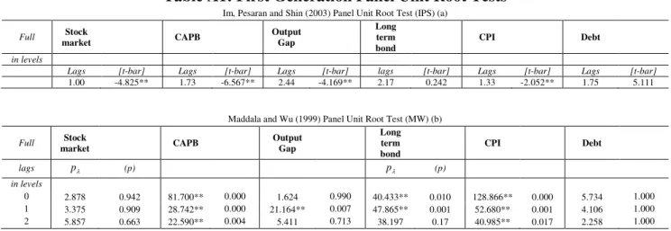
Table A1: First Generation Panel Unit Root Tests

Im, Pesaran and Shin (2003) Panel Unit Root Test (IPS) (a)

Full Stock

market CAPB

Output Gap

Long term bond

CPI Debt

in levels

Lags [t-bar] Lags [t-bar] Lags [t-bar] lags [t-bar] Lags [t-bar] Lags [t-bar]

1.00 -4.825** 1.73 -6.567** 2.44 -4.169** 2.17 0.242 1.33 -2.052** 1.75 5.111

Maddala and Wu (1999) Panel Unit Root Test (MW) (b)

Full Stock

market CAPB

Output Gap

CPI Debt

lags p (p) p (p)

in levels

0 2.878 0.942 81.700** 0.000 1.624 0.990 40.433** 0.010 128.866** 0.000 5.734 1.000 1 3.375 0.909 28.742** 0.000 21.164** 0.007 47.865** 0.001 52.680** 0.001 4.106 1.000 2 5.857 0.663 22.590** 0.004 5.411 0.713 38.197 0.17 40.985** 0.017 2.258 1.000

Notes: (a) We report the average of the country-specific “ideal” lag-augmentation (via AIC). We report the t-bar statistic, constructed

as _ _ 

i it N bar

t (1/ ) (tiare country ADF t-statistics). Under the null of all country series containing a nonstationary process this

statistic has a non-standard distribution: the critical values are -1.73 for 5%, -1.69 for 10% significance level – distribution is approximately t. We indicate the cases where the null is rejected with **. (b) We report the MW statistic constructed as

 

 2 ilog(pi)

p_ (piare country ADF statistic p-values) for different lag-augmentations. Under the null of all country series

containing a nonstationary process this statistic is distributed 2(2 )

N

 . We further report the p-values for each of the MW tests.

Table A2: Second Generation Panel Unit Root Tests

Pesaran (2007) Panel Unit Root Test (CIPS)

Full Stock

market CAPB

Output Gap

CPI Debt

lags p (p) p (p)

in levels

0 -0.275 0.391 -4.990** 0.000 2.313 0.990 -0.152 0.440 -1.295** 0.098 0.394 0.653 1 -0.197 0.422 -3.347** 0.000 -0.536 0.296 -0.063 0.475 0.095 0.538 1.278 0.899 2 0.919 0.821 -2.546** 0.005 0.473 0.682 1.268 0.898 -0.662 0.254 2.523 0.994