Enhancing Science and Mathematics Education with Computational
Modelling
Rui Gomes Neves & Vítor Duarte Teodoro
Unidade de Investigação Educação e Desenvolvimento (UIED), Departamento de Ciências Sociais Aplicadas (DCSA), Faculdade de Ciências e Tecnologia, Universidade Nova de Lisboa
rgn@fct.unl.pt & vdt@fct.unl.pt Abstract
The development of knowledge in science and mathematics involves modelling processes where theory, experiment and computation are dynamically interconnected. For education in these fields to be in contact with their rapid progress and closer to the nature of research, it is crucial that both curricula and learning environments from high school to university manifest effectively a balanced interplay between theoretical, experimental and computational elements. We present an approach to improve the integration process of computational modelling in the science and mathematics high school and university curricula while respecting the cognitive balance between theoretical aspects, experimentation and scientific computation. As strategy, we propose the creation of learning activities built around exploratory and expressive computational modelling experiments which are presented in digital documents where the fundamental concepts and problem solving processes are explained using interactive text, images and embedded movies. To design the activities, special emphasis is given to cognitive conflicts in the understanding of scientific and mathematical concepts, to the manipulation of multiple representations of mathematical models and to the interaction between analytical and numerical solutions. We discuss illustrative examples constructed with Modellus which are relevant for the high school and undergraduate university curricula in mathematics and physics
.
Keywords: computational modelling, science and mathematics education, cognitive processes 1. Introduction
Science is a historically evolving structure of knowledge, based on hypothesis and models that generate theories, which aims to describe the composition, architecture and dynamics of the universe. Fundamental characteristics of science are the abstract nature of scientific concepts, methods and reasoning, the fact that their precise and operational descriptions are written in the language of mathematics and the requirement that scientific models and theories must lead to results which are consistent with systematic and reliable experiments (see, e.g., Chalmers, 1999; Crump, 2001; Feynman, 1967). The creation of scientific knowledge is a complex cognitive process where interactions between individual and collective reflections lead to the development of modelling actions which involve a balance between theory, experiment and computation (Blum, Galbraith, Henn & Niss, 2007; Neunzert & Siddiqi, 2000; Schwartz, 2007; Slooten, van den Berg & Ellermeijer, 2006). This is a process with a strong mathematical character because scientific modelling has the objective to find, interpret and validate approximate representations of systems, which are defined by sets of concepts whose specifications and relation mechanisms are described using mathematical entities and operations. In this context, computational modelling plays a key role in the expansion of the science cognitive horizon for allowing more calculation and visualization power in the exploration of the universe. This important role is extended to mathematics and the corresponding exploration of abstract worlds, and also to technology and engineering.
The close connection between science and mathematics, the deep abstract nature of both fields and their historical dependence are important factors which make science and mathematics intrinsically difficult subjects to learn and to teach. Although it is clear that this degree of cognitive difficulty is independent of the use of computational knowledge and technologies, it is likewise clear that science and mathematics education should be as close as possible to the nature and progress of the research processes in science and mathematics as well as to the rapid development of technology. To effectively implement this view of science and mathematics education, it is crucial to achieve an early integration of computational modelling in learning environments which reflect the multiple
components of research (Ogborn, 1994). However, even in technologically advanced countries, the integration of research inspired learning environments, computers, computational knowledge and software has not yet been fully accomplished in the science and mathematics curricula designed for high school and undergraduate university levels. As a consequence, the majority of these curricula are outdated and students tend to feel that what they learn is detached from the real world. This contributes to the development of negative opinions about science and mathematics education and is a factor leading to an increase in student failure.
The general physics curricula for first year undergraduate university students are illustrative examples of this problem. In general, the corresponding courses follow a traditional lecture plus laboratory instruction approach and cover a large number of physics topics that students find particularly difficult. The choice of pedagogic strategy, the number and content of the physics topics and the type of examples chosen to apply the fundamental concepts and methods is usually independent of the specific major. Often, the mathematical and physics knowledge are not appropriately connected. Modelling activities, involving computational knowledge or not, are generally absent from these courses. Hence, the majority of students are unmotivated passive listeners of the theoretical lectures which, without much thought, try to memorize formulas to solve typical exam problems. Their knowledge is weak and highly fragmented both in physics and mathematics. Consequently, the number of students that fail on the course examinations is usually very high and many of those that eventually succeed manifest persistent weaknesses in their understanding of elementary physics (Halloun & Hestenes, 1985; Hestenes, 1987; Hestenes, Wells & Swackhamer, 1992; McDermott, 1991).
Scientific research in physics education has shown that it is possible to improve the student learning results when they are guided to be involved in the learning activities in a way that approximates the kind of involvement scientists have in their research activities (Beichner et al., 1999; Handelsman et al., 2005; Keiner & Burns, 2010; Mazur, 1997; McDermott, 1997). This is not a surprising result. Scientific research in physics is an interactive and exploratory process of creation, testing and improvement of mathematical models that describe observable physical phenomena. It is this cognitive process that leads to an inspiring understanding of the mechanisms underlying the behaviour of physical systems. As a consequence, physics should be expected to be more successfully taught in research inspired learning environments where students are helped by teachers to work as scientists do. In this kind of class environment, knowledge performance is better promoted and common sense beliefs as well as incorrect scientific ideas can be more effectively fought.
The research process in science and mathematics is supported by a continuously evolving set of analytical, computational and experimental techniques. The same should be true for the corresponding learning processes, particularly in what concerns the role played by computational knowledge and technologies in the learning activities. Several attempts have already been made to introduce elements of computational modelling in science learning environments. Initially, the focus was on professional programming languages such as Fortran (Bork, 1967) and Pascal (Redish & Wilson, 1993). Although more recently this approach has evolved to Python (Chabay & Sherwood, 2008), it remains a fact that it demands students to develop extensive working knowledge of programming, a time consuming task which makes harder the process of learning the matters of science. The same happens with scientific computation software such as Mathematica or Matlab. To avoid overloading students with external programming notions or syntax, and focus the learning process on the relevant scientific and mathematical knowledge, several computer modelling systems have been created, for example, Dynamical Modelling System (Ogborn, 1985), Stella (High Performance Systems, 1997), Easy Java Simulations (Christian & Esquembre, 2007) and Modellus (Teodoro, 2002, 2004).
A balanced integration of computational modelling knowledge and technologies in learning environments for science and mathematics education is, thus, both a curricular and a technological innovation challenge. In this work, we present an approach which aims to improve the integration of computational modelling in the science and mathematics high school and undergraduate university curricula and, at the same time, to respect the cognitive balance between computation, experiment and theory. We argue that Modellus (a freely available software tool developed in Java which is able to run in all operating systems, see the software webpage at http://modellus.fct.unl.pt) can be used, and progressively enhanced, as a central element of this approach. Our strategy involves the creation of learning activities centred in exploratory and expressive computational modelling experiments which
are presented in digital documents explaining the fundamental concepts and problem solving processes using interactive text, images and embedded movies. The activities are designed to give special emphasis to the onset of cognitive conflicts in the understanding of scientific and mathematical concepts, to the manipulation of multiple representations of mathematical models and to the interplay between analytical and numerical solutions. These activity documents can be adopted as a whole or partially by high school and undergraduate university courses in science and mathematics. In addition, they can also be useful for the professional development of high school and university teachers, and may be easily adapted to e-learning courses, being complemented with online tests in standard formats. We discuss illustrative examples which are relevant for high school and undergraduate university curricula in mathematics and physics.
2. Learning science and mathematics, computational modelling and Modellus
The construction of scientific and mathematical knowledge requires unambiguously clear declarative, operational and conditional specifications of abstract concepts and of the relations existing among them. Crucially important for the understanding of the resulting models or theories is the interpretation and validation process which involves operational familiarization, stringent consistency requirements and a clear connection with the relevant referents, either in the observable universe or in abstract mathematical worlds (Reif, 2008). Due to more powerful calculation, exploration and visualization capabilities, computational knowledge and technologies can amplify the cognitive and motivation horizon of the learning process and lead to deeper operational familiarization, consistency awareness and connection with the appropriate referents. To be able to fulfil such an important role, computers, computational methods and software should be used not only to display text, images or simulations but as tools for modelling integrated in learning environments reflecting the exploratory and interactive nature of modern research. In addition, the computational modelling process should be focused on the meaning of models and avoid learning opacity factors such as too much programming and specific software knowledge.
Clearly, this educational challenge cannot be met by simply choosing a subset of programming languages and professional scientific computation software. It is necessary to develop computer software systems with computational modelling functionalities that contribute to a progressive growth of solid cognitive competencies in science and mathematics. In this context, Modellus stands out as a possible key computational modelling system because it is a domain general environment for modelling (Schwartz, 2007) with the following main advantages:
1) An easy and intuitive creation of mathematical models using standard mathematical notation.
2) The possibility to create animations with interactive objects that have mathematical properties expressed in the model.
3) The simultaneous exploration of multiple representations such as images, tables, graphs and animations.
4) The computation and display of mathematical quantities obtained from the analysis of images and graphs.
These features allow a deeper cognitive contact of models with their referents and a deeper operational exploration of models as objects which are simultaneously abstract, in the sense that they represent relations between mathematical entities, and concrete, in the sense that they may be directly manipulated in the computer.
As a domain general environment for modelling, Modellus can be used to design learning activities which involve the exploration of existing models and the development of new ones (Bliss & Ogborn, 1989; Schwartz, 2007). These modelling activities can be collaborative and can be conceived to emphasize cognitive conflicts in the understanding of scientific and mathematical concepts, the manipulation of multiple representations of mathematical models and the interconnection between analytical and numerical approaches to solve problems in science and mathematics. As much as possible, the modelling activities should consider realistic problems to maximize the cognitive contact between models and real world referents. This is a challenge because more realistic problems are generally associated with more complex analytic solutions which are beyond the analytic capabilities of high school or first to second year university students. With Modellus and numerical methods, which can be conceptually simpler and yet powerful, the interactive exploration of models for more
realistic problems can start at an earlier age, allowing students a closer contact with the model referents, an essential cognitive element to appreciate the relevancy and power of models, necessarily a partial idealized representation of their referents.
The development of this kind of computational modelling activities, in a way that is adequate to the various areas of science and mathematics, is bound to require a richer set of modelling functionalities which are not yet available in Modellus. This is a trigger for technological evolution which should be accomplished by a Modellus enhancement program. Currently under development and set to appear in forthcoming versions of Modellus are, for example, the following new functionalities: spreadsheet, data logging and curve fitting capabilities, advanced animation objects like curves, waves and fields, 3D animations and graphs, creation of a physics engine for motion and collisions, video analysis and cellular automata models.
The simultaneous development of new functionalities to meet appropriate teaching goals is important because it reduces the learning opacity factor associated with an unnecessary proliferation of tools. However, there is a learning stage where it is advantageous to allow diversity and complement Modellus with other available tools. Indeed, in research inspired learning environments one of the objectives is to make a progressive introduction to professional computation methods and software. For example, Excel is a general purpose spreadsheet where modelling is focused on the algorithms. In addition, it already allows data analysis from direct data logging. On the other hand, Mathematica and Matlab (or wxMaxima, a similar but freely available tool) have powerful symbolic computation capabilities. Using these different tools to implement the same algorithm is an important step to learn the meaning of the algorithm instead of the syntax of a particular tool. For more realistic simulations Modellus animations can be complemented, for example, with EJS.
3. Interactive PDF documents for interactive learning environments
To reflect the nature of research, the environments to learn science and mathematics with computational modelling should be adapted interactive engagement environments (Beichner et al., 1999; Keiner & Burns, 2010; Mazur, 1997; McDermott, 1997) where students are organized in collaborative groups of two or three, one group for each available computer. In these environments, the student teams are continuously helped in their own processes of exploring and solving the computational modelling problems posed in the learning activities. Whenever necessary, global discussions are conducted to keep the pace, to introduce new themes, to clarify any doubts on concepts, reasoning or calculations, and for students to present the results of their work.
An important element of these research inspired environments is the document concept to present the set of learning activities. In our approach, we propose the creation of digital PDF documents which explain the fundamental modelling ideas and problem solving processes using interactive text, images and embedded movies. To amplify their level of interactivity, these documents include free space to allow students to write and register in the document itself the results of their exploratory or expressive modelling actions, including all that is necessary to complement the document information, for example, text comments, schemes, images and internet searches. The use of these interactive digital documents is another opportunity to improve the students ICT skills, particularly those related to work presentation and communication. All learning documents, including evaluation tests, are to be made available online, for example, through the Moodle e-learning platform.
4. Computational modelling activities: examples from physics and mathematics
We have made a progressive application of our approach implementing a series of computational modelling activities built with Modellus in the 2008 and 2009 editions of the general physics course offered to first year biomedical engineering students at the Faculty of Sciences and Technology of the New Lisbon University (Neves, Silva & Teodoro, 2008, 2009 and 2010). For other educational applications and evaluation tests of Modellus as a tool for learning mathematical modelling with computers see, e.g., Araújo, Veit & Moreira (2008), Dorneles, Araújo & Veit (2008) and Teodoro (2002).
The course was split into lectures built around a set of key experiments where the general physics topics were first introduced, standard physics laboratories and computational modelling classes following our methodological approach. The general physics program offered to the
biomedical engineering students was based on Halliday, Resnick & Walker (1997), Tipler (1991) and Young and Freedman (2004), complemented with applications of physics to biology and medicine. Following its structure the computational modelling component covered eight basic themes in mechanics (Teodoro, 2006):
1) Vectors.
2) Motion and parametric equations. 3) Motion seen in moving frames.
4) Newton’s equations: analytic and numerical solutions. 5) Circular motion and oscillations.
6) From free fall, to parachute fall and bungee-jumping. 7) Systems of particles, linear momentum and collisions. 8) Rigid bodies and rotations.
In each computational modelling class of the course, the student teams worked on an interactive digital PDF document containing a small number of problems connected with easily observed real world phenomena, which was complemented by an online Moodle test where the answers to the document questions were inserted. Although this was an undergraduate university course, many of the program themes involved revision activities discussing physical and mathematical concepts at the high school level. In what follows we illustrate our computational modelling approach discussing a selected set of examples associated with this course which can be useful for both high school and early undergraduate university curricula in physics and mathematics.
Figure 1: Mathematical model and animation defining the magnitude, direction and the sum of two vectors. The direction angles are given in degrees in the navigation convention where the angle varies between 0 and 360 clockwise starting from the North or, in Modellus Oxy reference frames, from the positive Oy axis.
Let us start with vectors, the first theme of the general physics computational modelling course. A vector is an abstract mathematical entity defined by a magnitude and a direction. In physics it is used to describe many important quantities or measures, for example, the velocity, the acceleration or the force acting on a particle. Using Modellus students can create vectors in the animation workspace and directly interact with them to visualise and reify many of its abstract mathematical properties. Indeed, when a vector is created it is immediately possible see its scalar and vector components on the screen. By simply using the computer mouse to drag the tip of the vector, students can change its magnitude or its direction, and explore the effect on the scalar and vector components. Furthermore, introducing the vector coordinates as parameters and using Modellus predefined elementary functions, students can also be taught to construct mathematical models to define the magnitude and the direction of any vector, the sum and subtraction of vectors, the multiplication of a vector by a scalar as well as the scalar and vector product of vectors (see figure 1). Students can then start modelling physical or geometrical problems involving vectors and vectors operations.
A simple example requiring the definition of vector directions and the sum of position vectors is that of a boat trip (see figure 2). Suppose a boat leaves a port following the direction 045 (in the navigation convention, see caption in figure 2). After sailing for 5 nautical miles, the boat changes direction and continues to move eastwards for 10 more miles. Considering 2 significant figures, find out what is the final distance between the boat and the point of departure. Where is the boat, if the port is taken as the reference point and what is the total distance travelled by the boat? With this modelling problem, students can be made aware of potential difficulties in using trigonometric functions to
define direction angles in the navigation convention, such as different conventions to define the angles and how the angle trigonometric formula change with the direction quadrant. The possibility to correct the models and simultaneously visualise the effect of the change in the vectors of the animation is a powerful cognitive aid to solve this kind of possible modelling problems. After completing this activity, students can use Modellus to make iterative extensions and continue the boat trip, determining at each intermediate point the localization and total distance travelled. A possible modelling activity starts with the visualisation of a movie embedded in the PDF document and showing a boat trip with several direction changes in a Modellus animation. After seeing the movie the students are guided to construct a model that reproduces the motion. In this way, students can be introduced to the concept of approximate trajectory, and by seeing it on the animation screen they can construct a deeper connection with the corresponding real world referent.
Figure 2: The model and animation for the boat trip. The final distance to the port is 14 miles and the direction 75.4 degrees. In this journey, the boat travelled 15 miles.
Figure 3: The model and animation for the geometric problem about the circumference at the straight line which involves the scalar product of two vectors.
An example of a purely geometrical problem involving vectors and their scalar product is the following: consider a point P, say P = (50, 70), that is located in a circumference centred in the origin of a Cartesian reference frame. Find the parametric and Cartesian equations of the straight line that passes through P and is tangent to the circumference. Show that Q = (-125, 195) is on the straight line and determine the corresponding equation parameter k. In this activity, students start by watching a movie of the Modellus animation and then are helped to construct the mathematical model, reproduce the animation and solve the problem (see figure 3). The animation is constructed with two perpendicular vectors, two geometrical objects, one representing the circumference and the other representing the straight line, a particle to represent the point Q and a level indicator for the equation parameter k. A pen is included to draw the graph of the straight line. In this model the coordinates of the vector pointing to P are independent variables. As a consequence, by dragging the tip of this vector, students can solve the problem for an arbitrary point P while simultaneously visualising the changes in the animation geometry. The possibility of exploring at the same time several different representations of the model (animation, graph and the mathematical model analytical equations)
allows students a much stronger and concrete cognitive connection with the abstract mathematical model and their entities.
The vector modelling activities involving real world physics problems can help students to understand that vectors are mathematical objects which are used to represent physical quantities that require both a magnitude and a direction to be completely specified. As the position vector, the velocity is another example. The velocity is a fundamental vector quantity which measures the instantaneous rate of change of the position with time. In a rectilinear and uniform motion, the velocity is constant and the position vector changes linearly with time. This type of motion can be modelled with Modellus if the coordinates of the position vector are associated with the corresponding parametric functions. Students can explore interactively several rectilinear and uniform motions on the plane using mathematical models with parametric equations, graphs of the coordinates as functions of time and particle animations representing the motion trajectory (see figure 4). The possibility to see, simultaneously, trajectories and different coordinate graphs is a powerful aid in helping them to manipulate, distinguish and correctly interpret these different representations of this kind of models.
Figure 4: Mathematical model and animation for a rectilinear and uniform motion showing that the graphs of the coordinates as functions of time are clearly not to be confused with the particle trajectory.
At the end of the classes covering vectors, uniform motion and parametric equations, students showed ability to complete computational modelling activities requiring knowledge on how to characterise displacement vectors and velocities by their magnitude, direction and Cartesian coordinates as well as knowledge about the parametric equations of motion. For example, all the student groups were able to develop models to solve and animate the following problem about the motion of a car (see figure 5): a car is detected 4 km away when is moving to the east. Seven minutes later the car is found 10 km away in the direction 035. What is the distance travelled by the car between the two detection points? Where does the displacement vector points? Assuming that the motion is uniform and rectilinear, determine the velocity of the car.
Figure 5: Modelling the motion of a car. The car travelled 8.37 km approximately in the direction 012 at a speed equal to 72 km/h.
The third theme of the general physics course was relative motion. With Modellus it is possible to create cognitive conflicts to help students realise that observers in reference frames moving with constant velocities can have very different views of a same motion. These different views are in fact related by a Galilean velocity transformation, making this a concrete application of an important mathematical concept, a linear vector transformation (see, e.g., Apostol (1975) and Courant & John (1989)). For example, with Modellus students can model and construct an animation representing the motion of a swimmer in a river with a downstream current (see figure 6). When the swimmer tries to move up stream with the same speed as the downstream current it does not move at all relative to an observer on the river margin. However, for an observer on a boat dragged by the current, the swimmer moves up stream with a speed equal to that of the current. For a student that is not thinking in terms of the velocity transformation kinematics this comes as a surprise, a cognitive conflict due to the wrong expectation that if the swimmer is moving in one frame then it will also be moving in another frame.
Figure 6: Modelling the motion of swimmer in river with a current, an example of relative motion and of the application of a Galilean velocity transformation.
At the end of this theme, students groups were able to successfully explore with Modellus other similar problems, for example, a boat crossing a river with a current (see figure 7). A boat tries to cross a river which has a current characterised by the velocity vector (10, -3) knots. Assume that the sailor verifies that the velocity relative to the water is (0, 10) knots. What is the velocity of the boat measured by a GPS device? If the velocity measured by the GPS is (0, 12) knots, what is the velocity relative to the river water? Students were also challenged to plan a crossing of the river Tejo from Almada to Lisbon along the 25 de Abril bridge when the tide is rising (see figure 8). Another example is the modelling of the motion of a plane in windy conditions. In this set of activities, the interactive modelling process with Modellus was important to make students more aware that many different, everyday life physical situations can be explained using the same mathematical model.
Figure 7: Modelling a boat crossing a river with a current. When the current velocity is (10,-3) knots and the velocity measured by the GPS is (0, 12) knots, the velocity relative to the water is (-10, 15) knots.
To finish the first part of the course, students modelled situations applying Newton’s equations of motion. The starting question was: what must happen for the velocity to change during motion? If
the velocity is changing then there must be an acceleration vector, measuring the instantaneous rate of change of the velocity with time, and at least one applied force. According to Newton’s second law of motion, the acceleration vector is obtained dividing the sum of all the forces that act on the particle by the mass of the particle. If there are no net forces then there is no acceleration and the velocity is constant. This is the statement of Newton’s first law of motion or law of inertia. If the acceleration is known we can use Modellus to calculate the velocity and the position of a particle. If the acceleration is constant the exact analytical solution is easy to determine and is well known. This makes uniformly accelerated motions ideal modelling stages to introduce simple numerical methods like the Euler and the Euler-Cromer methods. Students can then compare the analytical and numerical solutions of Newton’s equations of motion, a notable example of a system of first order ordinary differential equations which are also discussed in early undergraduate mathematics courses (see, e.g., Apostol (1975) and Courant & John (1989)).
Figure 8: Using the Galilean velocity transformation model to plan a boat trip on the river Tejo. A concrete problem is the following (see figure 9): suppose that the net force applied to a particle with mass equal to 1 kg is given by the vector (16, 0) N and that the particle starts at the origin of the reference frame with a velocity equal to (-55, 0) m/s. Applying the Euler method, find out when the velocity is zero, and the acceleration as well as the position of the particle at that instant. The model animation is constructed with three objects: the particle, a vector representing the velocity attached to the particle and a vector representing the net force. Because the coordinates of the net force vector are independent variables and the model is iterative, students can change this vector at will and in real time control realistically the motion of the particle (see figure 10). In this way students can face and resolve another cognitive conflict: to break is not that different from accelerating, it is just to accelerate in the direction opposite to the direction of the velocity. They can also learn that the choice of a small time step is important to obtain a good simulation of the motion and that this is the same as determining a good numerical solution of the equations of motion. The corresponding acceleration, velocity and position time graphs can easily be drawn. By observing these graphical solutions students are led to realise that, contrary to the constant force example, these are solutions they cannot find analytically and that numerical methods are indeed a simple and powerful way of solving more realistic problems.
Figure 9: Solving Newton’s equations iteratively with the Euler method. The velocity vector is zero for
A similar numerical model with the Euler-Cromer method can be used to explore, for example, the problem of throwing of a ball into the air (see figure 11).
Figure 10: A motion generated interactively by dragging in real time the net force vector. The Euler solution was obtained using a time step equal to 0.01 s.
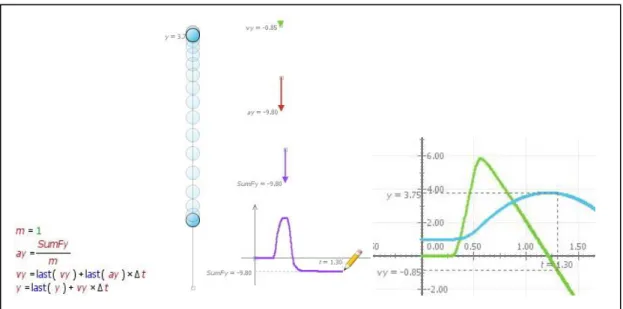
In this activity, students also interact with the net force vector applied to the ball and simulate the throw as well as the following motion under the earth’s gravity. In this example, an appropriate time step choice is very important to make a realistic throw. With the Modellus animation a good time step can be found by trial and error using the possibility of changing the mathematical model and immediately observe the effect of the correction in the animation. The same can be done with the appropriate scales for the animation objects and graphs. With the position and velocity time graphs, students can determine how long it takes for the ball to reach the highest point of the trajectory, what is the height of that point and when is the ball three metres up in the air. The students can also draw on the animation screen the vector diagrams representing the forces acting on the ball, the velocity and the acceleration during the whole motion. Finally, by observing the net force graph as a function of time, they can estimate the duration of the throw.
Figure 11: Throwing a ball with Modellus and the Euler-Cromer iterative Newton’s equations. The highest point of the trajectory is at y = 3.8 m, reached after 1.2 s. The ball is 3 m up in the air for t = 0.8 s and t = 1.6 s.
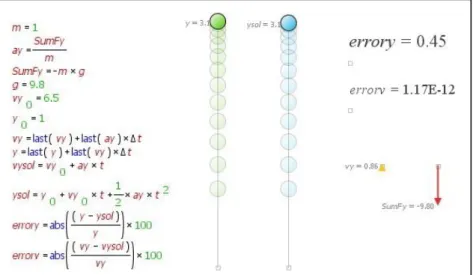
The next naturally following computational modelling activity is to compare the analytic solution for the motion just after the throw with the corresponding numerical solution obtained using the Euler method and the Euler-Cromer method (see figure 12). For the same sum of applied forces and the same initial conditions, students can verify that the analytic solution is indeed different from the numerical solutions and that there is always an error associated with the iterative approximations which can be quantified. In this particular example, students can note that the error is only present for the position and not for the velocity, since this quantity changes linearly with time.
Figure 12: Comparing the analytic solution and the Euler numerical solution of the ball throw.
5. Conclusions
In this paper we have presented a strategy to enhance the integration of computational modelling in the science and mathematics high school and undergraduate university curricula, which can display the cognitive balance existing between theory, scientific computation and experimentation in modern scientific and mathematical research. We have argued that this approach can be based on the creation of interactive engagement learning activities centred in exploratory and expressive computational modelling experiments, presented in digital documents which explain the fundamental concepts and problem solving processes using interactive text, images and embedded movies. These activity documents can be adopted as a whole or partially by high school and undergraduate university courses in science and mathematics. In addition, they can also be useful for the professional development of high school and university teachers, and may be adapted to e-learning courses. We have shown that Modellus can be a central system to implement this modelling strategy because it is designed as a domain general environment where both exploratory and expressive computational modelling can be developed, taking advantage of the following important cognitive features:
1) It is possible to create mathematical models using standard mathematical notation.
2) It is possible to create animations with interactive objects whose mathematical properties are visibly expressed in the model.
3) It is possible to make a simultaneous exploration of multiple representations, namely, images, tables, graphs and animations.
4) It is possible to compute and display mathematical quantities obtained from the analysis of images and graphs.
As concrete illustrative examples relevant for integration in both physics and mathematics high school and early undergraduate curricula, we have discussed a set of computational modelling activities associated to the general physics course we offered in 2008 and 2009 to the first year biomedical engineering students enrolled in the Faculty of Sciences and Technology of the New Lisbon University (Neves, Silva & Teodoro, 2008, 2009 and 2010). With these examples, we showed that the computational modelling activities with Modellus can be created to emphasise cognitive conflicts in the understanding of scientific and mathematical concepts, the manipulation of multiple representations of mathematical models and the interplay between analytical and numerical solutions.
In the field tests with the biomedical engineering students, the computational modelling activities with Modellus showed ability to identify and resolve many student difficulties in important physical and mathematical concepts of the general physics course. Crucial to achieve this was the possibility to have a real time visible correspondence between the animations with interactive objects and the object’s mathematical properties defined in the model as well as the possibility to analyse
simultaneously several different representations. Students were also able to work as authors of mathematical and physics models and their associated animations, not as simple browsers of computer simulations. In addition, students solved models with first order ordinary differential equations applying simple numerical methods and understanding the conceptual and operational differences existing between numerical solutions and analytical solutions. This is a strong indication that our approach is helpful to improve the learning process of mathematical models in science and mathematics education and it is supported by the student answers to the questionnaires given at the end of the courses (Neves, Silva & Teodoro, 2008, 2010). Indeed, globally, students reacted positively to the interactive computational modelling activities with Modellus, considering them to be important in the context of the biomedical engineering major. Students showed a clear preference to work in teams in an interactive engagement learning environment, if professors give adequate guidance and support. The computational activities with Modellus presented in digital PDF documents with embedded video guidance were also considered to be interesting and well designed. Finally, students found that Modellus was easy to learn and user-friendly.
Acknowledgements
Work supported by Unidade de Investigação Educação e Desenvolvimento (UIED) and Fundação para a Ciência e a Tecnologia (FCT), Programa Compromisso com a Ciência, Ciência 2007.
References
Apostol, T. (1975). Calculus, vol. 1 and 2, 2nd edition. San Francisco, USA: Wiley.
Araújo, I., Veit, E., & Moreira, M. (2008). Physics student’s performance using computational modelling activities to improve kinematics graphs interpretation. Computers and education, 50, 1128-1140.
Beichner, R., Bernold, L., Burniston, E., Dail, P., Felder, R., Gastineau, J., Gjertsen, M., & Risley, J. (1999). Case study of the physics component of an integrated curriculum. Physics Education
Research, American Journal of Physics Supplement, 67, 16-24.
Bliss, J., & Ogborn, J. (1989). Tools for exploratory learning. Journal of Computer Assisted learning, 5(1), 37-50.
Blum, W., Galbraith, P., Henn, H.-W., & Niss, M. (Eds.) (2007). Modelling and applications in
mathematics education. New York, USA: Springer.
Bork, A. (1967). Fortran for physics. Reading, Massachusetts, USA: Addison-Wesley.
Chabay, R., & Sherwood, B. (2008). Computational physics in the introductory calculus-based course.
American Journal of Physics, 76, 307-313.
Chalmers, A. (1999). What is this thing called science? London, UK: Open University Press.
Christian, W., & Esquembre, F. (2007). Modeling physics with Easy Java Simulations. The Physics
Teacher, 45 (8), 475-480.
Courant, R., & John, F. (1989). Introduction to Calculus and Analysis, vol. 1 and 2. New York, USA: Springer-Verlag.
Crump, T. (2002). A brief history of science, as seen through the development of scientific instruments. London, UK: Robinson.
Dorneles, F., Araújo, I., & Veit, E. (2008). Computational modelling and simulation activities to help a meaningful learning of electricity basic concepts. Part II - RLC circuits. Revista Brasileira de Ensino
da Física, v. 30, n. 3, 3308, 1-16.
Feynman, R. (1967). The character of physical law. New York, USA: MIT Press.
Halliday, D., Resnick, R., & Walker, J. (1997). Fundamentals of physics, extended fifth edition. New York, USA: Wiley.
Halloun, I., & Hestenes, D. (1985). The initial knowledge state of college physics students. American
Journal of Physics, 53, 1043-1048.
Handelsman, J., Ebert-May, D., Beichner, R., Bruns, P., Chang, A., DeHaan, R., Gentile, J., Lauffer, S., Stewart, J., Tilghmen, S. and Wood, W. (2005). Scientific Teaching. Science 304, 521-522.
Hestenes, D. (1987). Toward a modelling theory of physics instruction. American Journal of Physics, 55, 440-454.
Hestenes, D., Wells, M., & Swackhamer , G. (1992). Force concept inventory. The Physics Teacher, 30, 141-158.
High Performance Systems (1997). Stella, version 5. Hannover, NH: High Performance Systems. Keiner, L., & Burns, T. (2010). Interactive engagement: how much is enough? The Physics Teacher, 48, 108-111.
Mazur, E. (1997). Peer instruction: a user’s manual. New Jersey, USA: Prentice-Hall.
McDermott, L. (1991). Millikan lecture 1990: what we teach and what is learned–closing the gap.
American Journal of Physics, 59, 301-315.
McDermott, L. (1997). Physics by inquiry. New York, USA: Wiley.
Neunzert, H., & Siddiqi, A. (2000). Topics in industrial mathematics: case studies and related
mathematical models. Dordrecht, Holland: Kluwer Academic Publishers.
Neves, R., Silva, J., & Teodoro, V. (2008). Improving the general physics university course with computational modelling. Poster presented at the 2008 Gordon Research Conference, Physics research
and education: computation and computer-based instruction, Bryan University, USA.
Neves, R., Silva, J., & Teodoro, V. (2009 ). Computational modelling with Modellus: an enhancement vector for the general university physics course. In A. Bilsel & M. Garip (Eds.), Frontiers in science
education research (pp. 461-470). Famagusta, Cyprus: Eastern Mediterranean University Press.
Neves, R., Silva, J., & Teodoro, V. (2010). Improving learning in science and mathematics with exploratory and interactive computational modelling. In G. Kaiser, W. Blum, R. Borromeo Ferri & G. Stillman (Eds.), ICTMA14: Trends in teaching and learning of mathematical modelling, accepted for publication.
Ogborn, J. (1985). Dynamic modelling system. Harlow, Essex, UK: Longman.
Ogborn, J. (1994). Modelling clay for computers. In B. Jennison & J. Ogborn (Eds.), Wonder and
delight, Essays in science education in honour of the life and work of Eric Rogers 1902-1990 (pp.
Redish, E., & Wilson, J. (1993). Student programming in the introductory physics course: M.U.P.P.E.T. American Journal of Physics, 61, 222-232.
Reif, F. (2008). Applying cognitive science to education: thinking and learning in scientific and other
complex domains. Cambridge, USA: MIT Press.
Schwartz, J. (2007). Models, Simulations, and Exploratory Environments: A Tentative Taxonomy. In R. A. Lesh, E. Hamilton & J. J. Kaput (Eds.), Foundations for the future in mathematics education (pp. 161-172). Mahwah, NJ: Lawrence Erlbaum Associates.
Slooten, O., van den Berg, E., & Ellermeijer, T. (Eds.) (2006). Proceedings of the International Group
on Research on Physics Education (GIREP) 2006 conference: modelling in physics and physics education. Amsterdam, Holland: European Physical Society.
Teodoro, V. (2002). Modellus: learning physics with mathematical modelling. PhD Thesis. Lisboa, Portugal: Faculdade de Ciências e Tecnologia, Universidade Nova de Lisboa.
Teodoro, V. (2004). Playing newtonian games with Modellus. Physics Education, 39, 421-428.
Teodoro, V. (2006). Embedding Modelling in the General Physics Course: Rationale and Tools. In Slooten, O., van den Berg, E. and Ellermeijer, T. (Eds.), Proceedings of the International Group of
Research on Physics Education 2006 Conference: Modelling in Physics and Physics Education (pp.
48-56). Amsterdam, Holland: European Physical Society.
Tipler, P. (1991). Physics for scientists and engineers, third edition, extended version. New York, USA: Worth Publishers.