CAPM: AN APPLICATION TO THE PORTUGUESE
COMPANIES IN THE RETAIL SECTOR
Diana Patrícia Correia Batista
Dissertation submitted as partial requirement for the conferral of Master in Business Administration
Supervisor:
Professor Doutor José Joaquim Dias Curto, Associate Professor
ISCTE Business School, Quantitative Methods for Management and Economics Department
CA P M : A N AP P L IC AT ION T O TH E P O R TU G U ES E C O M P A N IES I N TH E R ETA IL S E C TO D ian a P at rí ci a C or re ia B at is ta
The objective of this study is to estimate the CAPM for the two Portuguese retail companies listed in the PSI-20 (JMT and SON) and assess how the two of them evolve regarding the Portuguese market index.
This study covered sixteen years (pre and post-subprime crisis) and, based on estimation results, we established a comparison between the relation of each company with the PSI-20. We also analysed the differences before and after the 2008 financial crisis. For this purpose, the estimation of α and β coefficients was done by using the OLS method, and the adequacy of the model was checked by verifying the statistical significance of the regression coefficients and the fulfilment of the OLS assumptions.
Finally, the main conclusion is that the two companies tend to behave differently concerning the Portuguese market index. All the beta estimates were statistically significant, meaning that changes in the PSI-20 returns will influence the changes on each company’s returns, which is in line with the CAPM. However, except for two periods for JMT, the alpha estimates were statistically significant, meaning that there were additional factors other than the market risk premium that explained the expected value of excess returns. We could also note that the expected returns for JMT went from a negative value (pre-crisis) to a positive value (post-crisis), while for SON there was a decline in the alpha value.
Keywords: Jerónimo Martins (JMT), Sonae (SON), PSI-20, Market risk JEL codes: C20, G12
O objetivo deste estudo é estimar o CAPM para as duas empresas de distribuição portuguesas que estão listadas no PSI-20 (JMT e SON) e avaliarmos como é que elas evoluem em relação ao índice de mercado português.
Este trabalho abrangeu um período de dezasseis anos (pré e pós-crise do subprime) e, com base nos resultados das estimativas, fizemos uma comparação entre a relação de cada empresa com o PSI-20. Posteriormente analisámos as diferenças entre o antes e o após da crise financeira de 2008. Para isso, estimámos os coeficientes α e β através do método OLS e a adequação do modelo foi verificada através da significância estatística dos coeficientes da regressão e do cumprimento das hipóteses do método.
Por fim, a principal conclusão é que as duas empresas tendem a comportar-se de maneira diferente em relação ao índice de mercado português. Todas as estimativas do beta são estatisticamente significativas, o que significa que as mudanças na rendibilidade do PSI-20 influenciam as mudanças nos retornos de cada empresa, o que está alinhado com o CAPM. No entanto, com exceção de dois períodos para a JMT, as estimativas para o alfa são estatisticamente significativas, o que significa que, além do prémio de risco de mercado, há outros fatores que explicam o valor esperado dos retornos em excesso. Também pudemos observar que os retornos esperados para a JMT passaram de um valor negativo (pré-crise) para um valor positivo (pós-crise), enquanto para a SON houve um declínio no valor de alfa.
Palavras-Chave: Jerónimo Martins (JMT), Sonae (SON), PSI-20, Risco sistemático Códigos JEL: C20, G12
1. Introduction ... 1
2. Literature review ... 4
2.1. PSI-20 index ... 4
2.2. Jerónimo Martins ... 6
2.3. Sonae ... 6
2.4. The subprime crisis ... 7
2.5. Euribor ... 9
2.6. Risk ... 9
2.7. Return ... 10
2.8. Efficient Market Hypothesis ... 10
2.9. Modern Portfolio Theory ... 12
2.10. Capital Asset Pricing Model (CAPM) ... 13
2.11. Beta coefficient ... 17
3. Data and methodology ... 21
4. Results ... 29
4.1. Correlation Analysis ... 29
4.2. Estimation and statistical significance of the regression coefficients ... 31
4.3. Analysing the systematic risk ... 34
4.4. RESET test ... 36
4.5. Linearity ... 38
4.6. Normality of the errors ... 39
4.7. Homoscedasticity of the errors ... 42
4.8. No autocorrelation ... 45
5. Discussion results ... 48
6. Conclusions ... 55
Table 2 Correlation significance test ... 30
Table 3 Estimates and significance tests for alpha coefficient Period 1 ... 31
Table 4 Estimated alpha coefficients Period 2 ... 31
Table 5 Estimated alpha coefficients Period 3 ... 32
Table 6 Estimated beta coefficients Period 1 ... 33
Table 7 Estimated beta coefficients Period 2 ... 33
Table 8 Estimated beta coefficients Period 3 ... 33
Table 9 Estimated equations for Jerónimo Martins ... 34
Table 10 Estimated equations for Sonae ... 34
Table 11 Coefficient of Determination Period 1 ... 34
Table 12 Coefficient of Determination Period 2 ... 35
Table 13 Coefficient of Determination Period 3 ... 35
Table 14 P-values associated to the RESET test ... 36
Table 15 Kurtosis and Skewness Coefficients Period 1 ... 40
Table 16 Kurtosis and Skewness Coefficients Period 2 ... 40
Table 17 Kurtosis and Skewness Coefficients Period 3 ... 40
Table 18 White test period 1 ... 43
Table 19 White test period 2 ... 43
Table 20 White test period 3 ... 44
Table 21 White Standard Errors Jerónimo Martins Period 1 ... 44
Table 22 White Standard Errors Sonae Period 1 ... 44
Table 23 White Standard Errors Jerónimo Martins Period 2 ... 44
Table 24 White Standard Errors Sonae Period 2 ... 44
Table 25 White Standard Errors Jerónimo Martins Period 3 ... 45
Table 26 White Standard Errors Sonae Period 3 ... 45
Table 27 Breusch-Godfrey test Period 1 ... 46
Table 28 Breusch-Godfrey test Period 2 ... 46
Table 29 Breusch-Godfrey test Period 3 ... 46
Table 30 Newey-West standard errors Sonae Period 3 ... 47
Figure 2 Scatter Plot JMT, SON and PSI-20 Period 2 ... 29
Figure 3 Scatter Plot JMT, SON and PSI-20 Period 3 ... 29
Figure 4 Weight of the systematic and non-systematic risk in total risk Period 1 ... 35
Figure 5 Weight of the systematic and non-systematic risk in total risk Period 2 ... 36
Figure 6 Weight of the systematic and non-systematic risk in total risk Period 3 ... 36
Figure 7 Graphical Representation of the Residuals of JMT and SON against the PSI-20 Period 1 ... 37
Figure 8 Graphical Representation of the Residuals of JMT and SON against the PSI-20 Period 2 ... 37
Figure 9 Graphical Representation of the Residuals of JMT and SON against the PSI-20 Period 3 ... 37
Figure 10 Residuals vs Predicted values period 1 ... 38
Figure 11 Residuals vs Predicted values period 2 ... 38
Figure 12 Residuals vs Predicted values period 3 ... 38
Figure 13 Normality Q-Q plot period 1 ... 39
Figure 14 Normality Q-Q plot period 2 ... 39
Figure 15 Normality Q-Q plot period 3 ... 39
Figure 16 Scale Location Plots Period 1 ... 42
Figure 17 Scale Location Plots Period 2 ... 42
Figure 18 Scale Location Plots Period 3 ... 43
Figure 19 Jerónimo Martins' returns Period 11 ... 48
Figure 20 Sonae's returns Period 1 ... 48
Figure 21 PSI-20' returns Period 1 ... 48
Figure 22 EBIDTA for JMT and SON (source: values obtained from the financial reports of JMT and SON) ... 51
ЕМН – Efficient Market Hypothesis
Euribor – Euro Interbank Offered Rate
GDP – Gross Domestic Product
JMT – Jerónimo Martins
OLS – Ordinary Least Squares Method
PSI – Portuguese Stock Index
SML – Security Market Line
1. Introduction
The objective of this dissertation is to estimate the CAPM (Capital Asset Pricing Model) for the two listed Portuguese companies in the retail sector: Sonae SGPS SA (SON) and Jerónimo Martins SGPS SA (JMT) by using a regression model to estimate and analyse the specific and the systematic risk (beta) of the stocks of these two companies.
The companies that are the subject of the study – Jerónimo Martins and Sonae – are the two largest and more important Portuguese companies in the retail sector and they are listed in the Portuguese stock market (PSI-20 index).
The retail sector encompasses the economic activity that connects producers and consumers by making business transactions through entities like supermarkets and grocery stores, among others. Through these transactions and logistics operations, these entities meet the costumers’ needs by providing them products or services in the most convenient and efficient time, place and way (Ferreira, 2011). This sector is also relevant because it is the second widest sector in the PSI-20 index and, together, the two companies have a weight of 14,97%.
Among others, regression analysis is useful and commonly used to forecast future economic conditions; to determine the relationship between two or more variables; and to understand how one variable may change concerning another variable.
Assessing the relationship between risk and return is important when it comes to corporate finance. The CAPM is the most commonly used model to estimate the returns of the assets and to evaluate and predict the market risk of stocks; to evaluate companies by determining the cost of capital; and to help with management functions. Despite the clear limitations of this model, namely being very restrictive, the alternative models do not show higher forecasting ability, they are more complicated to use and require more data.
The research question is: “How does the Portuguese market influence the return of the two stocks of the retail sector?”. What is the relation between the Portuguese stock
market index and these two companies? Are they related? Do they evolve in the same way as the PSI-20 index or in opposite ways?
This study will cover a time range of 16 years and we will divide it between a before and an after the financial crisis of 2008. The year 2008 was characterized by the subprime mortgage crisis, with the worsening of the macroeconomic environment and volatility of the international financial markets. With the crisis, the confidence in the markets and banks was affected, which generated an environment of uncertainty.
There was a break in the economic growth, which translated into a lowering of the international trade rate, that went from 7.2% in 2007 to 4.6% in 2008. Other impacts of the crisis were the increase in unemployment, lower prices in stock markets, less consumption and less investment, which negatively affected the countries’ GDP (Financial report Jerónimo Martins, 2008).
The present study will be an empirical study that might be helpful for parties who are interested in the market, such as investors, by providing some directions and leads. This model also allows company managers to determine the rate of return on investments that the company will need to have to match investors' expectations.
For instance, by looking at the beta estimate, they will know that if the beta is higher than 1, the stock price will be more volatile than the market price; and that, conversely, if the beta is smaller than 1 it means that the stock price is less volatile than the market price. Thus, investors who have risk aversion should invest in stocks with low betas, while investors who prefer taking more risk and possibly win a higher return should invest in stocks with higher betas.
In order to achieve these objectives, this dissertation was divided into five chapters:
In the first one, we began with the introduction of the paper.
In the second chapter, we have a literature review. We started by introducing the two companies that are subject to the study, as well as the Portuguese market index. Then, we introduced the concepts of risk, return and beta, since they are important to understand the CAPM. In this chapter, we also studied important works in finance, such as the
Efficient Market Hypothesis and the Markowitz Portfolio Theory and finally the CAPM model, while describing its assumptions and properties. Since we divided the time length of the period covered in the study into pre and post-subprime crisis, we also explored the crisis in this chapter.
In the third chapter, the data and methodology used throughout our study were described.
In the fourth chapter, we presented the results of the correlation analysis, the estimation and statistical significance of the regression coefficients, the systematic risk, the RESET test, and the tests for the linearity, the normality, the homoscedasticity and no autocorrelation of the errors.
In the fifth chapter, we analysed and discussed the results obtained in the previous chapter and, finally, the main conclusions were presented in the last chapter.
2. Literature review
2.1. PSI-20 index
Euronext is the largest group of stock markets in the world, where more than 100 billion euros per day are traded. It is used in Europe and the United States to trade shares, bonds and commercial paper and it is the leading pan-European operator with the Paris, Amsterdam, Brussels and Lisbon stock exchanges.
The Lisbon Stock Exchange was established in 1769 and more than 200 years later, on 31 December 1992, the PSI-20 (Portuguese Stock Index) was founded, being the main index of Euronext Lisbon. It is vastly used to track the performance of the Portuguese stock market, as it shows how 18 to 20 most actively traded shares listed on Euronext Lisbon behave. Its purpose is to serve as a benchmark of the evolution of the Portuguese stock market (Euronext, 2003).
Due to its characteristics, the market has been selecting the PSI-20 index to help structured products whose profitability depends on the behaviour of the Portuguese stock market (Euronext, 2003).
To calculate the price index, the following formula is used:
It = ∑ = #$,&'$,&(+$,&)$,&*$,& &
,
-./ (1)
Where:
§ It is the value of the PSI-20 index on day t
§ t is the time of calculation
§ N is the number of constituent shares in the index
§ Qi,t is the number of shares of equity of the company i on day t
§ Fi,t is the free Float Factor of share i
§ Ci,t is the price of the share i on day t
§ Xi,t is the current exchange rate on day t
§ dt is the index divisor on day t
The PSI-20 is comprised by the following companies: EDP, Jerónimo Martins, Banco Comercial Português, Galp Energia, NOS, Redes Energéticas Nacionais, The Navigator Company, Energias de Portugal Renováveis, Sonae, Altri, Semapa, Corticeira Amorim, CTT Correios de Portugal, Mota-Engil, Pharol, Ibersol, Sonae Capital and Ramada.
These companies can be organised by sectors, and the PSI-20 index encompasses the following 12:
§ Banks: Banco Comercial Português
§ Basic Resources: The Navigator Company, Semapa, Ramada § Construction and Materials: Mota-Engil
§ Financial Services: Sonae Capital § Food & Beverage: Corticeira Amorim
§ Industrial Goods and Services: Altri, CTT Correios de Portugal § Media: NOS
§ Oil and Gas: Galp Energia § Retail: Jerónimo Martins, Sonae § Telecommunications: Pharol § Travel and Leisure: Ibersol
§ Utilities: EDP, Redes Energéticas Nacionais, Energias de Portugal Renováveis
The retail sector is the second widest sector in the PSI-20 index, encompassing Sonae and Jerónimo Martins. Together, these companies represent 14,97% of the PSI-20 universe.
2.2. Jerónimo Martins
Jerónimo Martins was established in 1792, weighting 10,18% in the PSI-20 index. It is a group that is mainly focused on food distribution (representing more than 95% of the sales), but also works in specialized retail.
This company is placed in Portugal, Poland, and Colombia, with market leadership positions in the first two countries.
In Portugal, Pingo Doce (with 432 supermarkets) and Recheio (with 39 Cash & Carry and 3 platforms related to Food Service) are leaders in the Supermarket and Cash & Carry segments, respectively. In the specialized retail, Jerónimo Martins is operating Jeronymo, a chain of kiosks and coffee-shops with 22 points of sale and Hussel, with 24 stores, dedicated to chocolates and confectionery. The total sales in Portugal in 2018 were 4,8 billion euros.
Jerónimo Martins also owns Jerónimo Martins Agro-Alimentar (JMA), to ensure there is a supply of some strategic products in the areas of Dairy Products, Livestock (Angus beef) and Aquaculture (sea bass and gilt-head bream).
In Poland, the chain Biedronka operates in 2,900 stores. There is also a chain in the Health and Beauty sector, Hebe, which has 230 stores, and a drugstore chain HebeApteka. In 2018, the total sales in Poland were 11.898 million euros.
In Colombia, the Group owns Ara which has 532 stores, having reached 599 million euros in 2018.
2.3. Sonae
Sonae (Sociedade Nacional de Estratificados) is a multinational company that was founded in 1959, weighing 4,79% in the PSI-20 index.
It is located in 74 countries and operates in retail, financial services, technology, shopping centres, and telecommunications.
In the retail area, Sonae MC is the market leader of food retail, with several brands such as Continente, Continente Modelo and Continente Bom Dia, Meu Super, Bom Bocado, Bagga, Go Natural, Make Notes, Note!, ZU, Well’s and Dr. Well’s; in the specialized retail in sports and fashion, Sonae S&F is responsible for Sportzone, Berg Outdoor, Berg Cycle, Deeply, Zippy, Losan, MO and Salsa; in the specialized retail in electronics we have Worten and Worten Mobile; and finally, Sonae Retail Properties, that deals with the optimization of the management of its retail real estate portfolio.
Regarding financial services, Sonae FS is responsible for the "Universo” card, "Dá” card, Continente Money Transfer, cross-selling over store credit services and also the insurance broker MDS.
In the field of technology, Sonae IM manages a portfolio of tech-based companies linked to retail and telecommunications: WeDo Technologies, Bizdirect, S21sec, Inovretail, Bright Pixel, and Excellium.
Sonae Sierra also owns of 46 shopping centres spread across 11 countries and responsible for the management and/or leasing of 64 shopping centres.
Finally, in the telecommunications and entertainment area, NOS has a leading position in Pay TV, Next Generation Broadband services and in cinema film exhibition and distribution in Portugal.
2.4. The subprime crisis
Since we are splitting our regression between the period that preceded the collapse of Lehman Brothers and the period right after that happened, it is important to give a background about the subprime crisis.
The financial crisis of 2008 initially began in the United States of America, after the collapse of the speculative bubble in the housing market, and rapidly spread into other segments and countries.
At the beginning of the 2000s, the federal funds rate was lowered, which meant that banks were charging lower interest rates to other banks for lending them money. The result was high liquidity in global financial markets, facilitating mortgage financing (Ackermann, 2008).
With the easing of US monetary policy for a considerable time, more loans were being done, especially for home buyers. The “subprime” mortgages appeared: mortgages made by borrowers who could not really afford the houses, with high credit risk for the lenders. The interest rates for the mortgages were low, which allowed consumers to get big loans while having relatively low monthly payments. This eventually led to home prices rising exponentially, which brought confidence to investors – lenders were relying on the boom in US real estate markets to get bigger revenues.
Back in 2004, the first signs that foreseen what was about to happen started as the interest rates increased and housing prices started to fall. The real estate market began to stagnate: the real estate market was saturated, and with higher interest rates the mortgages became more expensive, so fewer people turned to new mortgages and fewer houses were being bought. Consequently, the prices of houses and real estate began to decline, and mortgages stopped being refinanced (Singh, 2019).
Several US banks linked to the subprime mortgages went bankrupt and investors began losing money. This was due to the rising in the interest rates that led to households with low income not being able to pay the mortgages. As a result, banks hesitated to lend to each other because they could not be sure if they would get the money back (Pritchard, 2019).
The trigger of this crisis, however, was the bankruptcy of the investment bank Lehman Brothers (the fourth-largest investment bank in the US) on September 15, 2008, after the Federal Reserve rejected financial aid to the institution. This had a huge impact since numerous jobs were lost and people were left unemployed, while a scenario of high
insecurity and volatility was installed, making people question whether such big financial institutions were reliable and if their money could be trusted in such institutions (Sraders, 2018).
As a consequence, all over the world, the crisis was manifesting itself. In Portugal, there was a significant slowdown in private consumption and a decline in demand that, together with financial difficulties, led to the supply exceeding the demand. The GDP growth then turned negative at the end of 2008 as unemployment increased, which negatively influenced the retail activity.
2.5.Euribor
Euribor (Euro Interbank Offered Rate) is an important reference rate at which twenty panel banks (the ones with the highest volume of business) from Europe borrow funds from one another and it is based on the average interest rates. In total, there are five different Euribor rates that have different maturities, ranging from one week to one year.
Euribor rates are an important benchmark for the price and interest rates of financial products such as interest rate swaps, interest rate futures, saving accounts and mortgages.
2.6. Risk
Risk and return are important aspects to have in consideration when making an investment decision.
For a good definition of risk, we can start by analysing the Chinese symbols for risk: the first, for “danger” and the second, for “opportunity”. That being said, the risk illustrates the relationship between the risk and returns: the higher the risk, “danger” that is taken, the higher the opportunity that might come from it: the returns. So, if an investor is being exposed to risk, he should be rewarded accordingly for taking it (Damodaran, 2015).
Risk can be defined as the standard deviation of the return, the possibility that the actual return from an investment will be different from the expected return (Omisore, Yusuf & Christopher, 2012). This deviation can occur for reasons that are either firm-specific or market-firm-specific, thus, risk can be divided in firm-firm-specific risks (risks that only affect the firm) and market risks (risks that affect all the investments).
To sum up, risk can be defined as the possibility of financial loss, the level of uncertainty that is associated with investment: the bigger the volatility of the returns, the bigger the risk.
2.7. Return
Returns are the main rewards when investing and can be divided into expected returns and realized returns. The expected returns are what the investor is hoping to receive when he invests while the realized returns are what the investor actually receives. Since the expected return is a prediction, it is not certain that it will be the same as the realized return (Omisore, Yusuf & Christopher, 2012).
2.8. Efficient Market Hypothesis
The Efficient Market Hypothesis (ЕМН) is the basis of most financial theories. The EMH started with Paul A. Samuelson but was formalized by Eugene F. Fama in the 1970s and it is still one of the most controversial areas in investment research. The random character of prices is explained as the consequence of rational behaviours. But what is an efficient market?
A capital market is said to be efficient if the actual prices of the assets reflect all the information available at a given moment (Fama, 1970) and if the prices adjust quickly and accordingly to new information (Reilly & Brown, 2012).
For Fama, what matters is the degree of efficiency, not whether the markets are fully efficient. Therefore, financial markets can have three forms of efficiency: weak, semi-strong and semi-strong, depending on the type of information that the prices of assets reflect at any given time.
The weak form is the most restricted set of information and indicates that the current prices reflect all the information given by historical prices, rates of return, trading volume data, among others.
The semi-strong form assumes that the prices adjust to all the public information available in the market, which includes historical data of the asset and relevant public information about the company (announcement of annual earnings, stock splits, etc.), its competitors and the economy in general. The semi-strong hypothesis encompasses the weak form hypothesis.
Finally, the strong form is the set that includes more information and indicates that the prices reflect all the information available that is known and relevant in the market (historical, public and private). This means that no investor has monopolistic access to relevant information in the formation of prices. The strong form encompasses both the weak form and the semi-strong form EMH.
Fama (1970) concluded that there was no relevant evidence against the hypotheses of weak and semi-strong form tests since the prices efficiently adjust to available public information. Regarding the strong form tests, the results are not as conclusive, the evidence is limited, and investors do not seem to have monopolistic access to price information.
Therefore, in an efficient market the assets are always traded at their fair value and their price reflects the information contained in one of the three forms, so, the investors cannot purchase undervalued assets or sell them for higher prices. The only way for an investor to get higher returns on the investments is by incurring in more risk.
2.9. Modern Portfolio Theory
The beginning of the development of theories that relate risk and return was the Modern Portfolio Theory (MPT), also commonly known as mean-variance analysis, which started with Harry Markowitz’s article: “Portfolio selection”, published in 1952 in the Journal of Finance.
This theory was formulated to be a tool that would help rational and risk-averse investors to choose optimal portfolios in terms of risk and return based on a given level of market risk. According to the Market Portfolio Theory “an investor selects a portfolio at time t - 1 that produces a stochastic return at t” (Fama & French, 2004).
One of the assumptions of this model is that investors only care about the mean and variance of their one-period investment return. The intention is to choose mean-variance-efficient portfolios that maximize the expected return on their investments, so they are willing to take more risk until a certain level, depending on their risk aversion to get the desired expected return (Fama & French, 2004).
Another assumption is that investors base their decisions solely on expected return and risk. To estimate the risk, investors use the variability of expected returns. Being risk-averse, when two investments have the same expected returns, investors tend to choose the one with less risk.
Markowitz helped to develop the idea that merely combining various individual securities that have appealing characteristics regarding risk and return does not necessarily lead to an optimal portfolio. In fact, to get a mean-variance efficient portfolio the investor also needs to consider the relationship among the investments (Reilly & Brown, 2012).
According to Markowitz, the risk of the investment could be reduced by diversifying the portfolio, however, it is not enough to simply invest in many securities. In short, the investor should opt by investing in assets with different types of risk or different kinds of industries instead of investing all in the same type of asset. Combining assets or portfolios
whose returns are not highly correlated should be preferred to minimize the total variance of the portfolio return, “don’t put all your eggs in one basket” (Markowitz, 1952).
By doing this, it is possible to get a mean-variance efficient portfolio – a portfolio which maximizes the expected return on each investment and minimizes the variance. This optimal choice is placed in the efficient frontier, which encompasses all of the best assets’ combinations. Here, for each given level of risk, the investor can choose the combination of securities that will maximize the expected return on each investment or, for a given level of expected return, to choose the portfolio that will minimize the risk (Fabozzi, Gupta, & Markowitz, 2002).
Because different investors will have different preferences regarding risk and return, different portfolio choices will occur among investors who, between this set of optimal portfolios, select the one that lies at the point of tangency between the efficient frontier and their highest utility curve. Investors will choose between investment alternatives considering the probability distribution of expected returns and pick the portfolio based on the relation between the expected return and its variance (Reilly & Brown, 2012).
To sum up, if there is no asset or portfolio of assets that give higher expected returns with the same risk (or lower), or lower risk with the same expected return (or higher), an asset or a portfolio of assets is considered to be efficient (Reilly & Brown, 2012).
2.10. Capital Asset Pricing Model (CAPM)
The Capital Asset Pricing Model (CAPM) is the method that is used to predict how the capital markets behave. This model of Sharpe (1964), Lintner (1965) and Mossin (1966) is based on the Modern Portfolio Theory, developed by Harry Markowitz (1959), and it came out of the necessity to build a market equilibrium theory of asset pricing under an environment of risk. This model explains how the price of an asset and its overall risk are related (Sharpe, 1964) by identifying a portfolio that must be mean-variance-efficient (efficient if asset prices are to clear the market of all assets) (Fama & French, 2004).
With the capital asset pricing model is possible to allow investors to evaluate not only the risk and returns for diversified portfolios, but also individual assets.
There are some assumptions associated with the asset pricing model, in particular:
1. Investors rely on the expected returns and risk to choose among portfolios, which is measured by the standard deviation and expected returns;
2. Investors are rational and risk-averse, which implies that they require more compensation for bearing more risk, and when choosing between two portfolios that are expected to have the same profitability, they opt for the one with the lowest standard deviation. They always try to invest along the efficient frontier (depending on individual risk and return preferences) and the main goal is to minimize the investment risk and to maximize its profitability;
3. If two portfolios have the same level of risk, investors will be more inclined towards the one with the highest expected return;
4. Investors have the same time interval (one month, one year…) for decision-making, in which the interest rate is fixed. That allows us to evaluate the investors' expectations and to establish comparisons between them;
5. Complete agreement: given market-clearing asset prices at t - 1, investors agree on the joint distribution of asset returns from t - 1 to t. (Fama & French, 2004);
6. Investors can borrow and lend any amount of money at a given riskless rate, which is the same for all investors and independent of the amount borrowed or lent (Fama & French, 2004);
7. Financial markets are perfect, efficient and they are in equilibrium. The investments are properly priced and reflect available information;
8. All assets are infinitely divisible, so investors can buy or sell fractions of any asset;
9. Investors can invest or finance themselves - without amount restrictions - at the risk-free rate, which is the same for all investors. Personal income taxation is assumed to be zero;
10. There are no limits on short-selling, so investors can sell short any number of shares without restrictions;
11. There are no taxation or transaction costs and no taxes on dividends;
12. There is no inflation or any change in interest rates or inflation is fully anticipated;
13. Investors can access all relevant information that may influence the future profitability of a company instantly and at an affordable cost;
14. There is no private information and, therefore, investors cannot find under or overvalued assets in the marketplace;
15. Investors have rational and homogeneous expectations about asset returns, they all have the same assessment about the distribution of the future value of any asset or portfolio.
Since the information of financial assets is freely accessible and the same to all investors, their homogeneous expectations are explained by their common beliefs about the joint probability distributions of future returns (i.e., means and covariances).
Many of the CAPM's assumptions are difficult to observe under the actual conditions of world economies. As we know, real markets are not characterized by an absolute degree of efficiency, so different investors will have different preferences, and taxes and
transaction costs have a significant impact when building a portfolio. For these reasons, several assets that are available in the market are not in a straight line.
However, the assumptions are not sufficiently strict to invalidate the model. In fact, they are useful to describe a financial model and its practical applications.
The CAPM generates the following model:
𝐸 (𝑅𝑖) = 𝑅𝑓 + β𝑖 [𝐸 (𝑅𝑚) - 𝑅𝑓] (2)
Where:
▪ 𝐸 (𝑅𝑖) is the expected rate of return on the asset i;
▪ 𝑅𝑓 is the interest rate of a risk-free asset (Risk-free rate);
▪ β𝑖 is the systematic risk of asset i concerning the market, it indicates the relationship between changes in the price of the stock i and changes in the general market index;
▪ 𝐸 (𝑅𝑚) is the market yield rate of risky assets, the expected return on market
portfolio;
▪ 𝐸 (𝑅𝑚) – 𝑅𝑓 is the market risk premium.
With this equation, one can understand that the expected return on an asset i is equal to the risk-free interest rate, Rf, plus a risk premium (the asset’s market beta, β𝑖, times the premium per unit of beta risk, E(RM) - Rf).
This model shows that the expected return of stocks is equal to the sum of the risk-free rate and risk compensation by measuring the covariance between the rates of return of a security and the market portfolio rates of return.
As we can see, to use the model we need three inputs: the risk-free rate; the expected market risk premium; and the β of the asset under appreciation.
The risk-free rate is the rate of return that a risk-free investment would give, it is the expected return on assets that have market betas equal to zero, which means their returns
are uncorrelated with the market return. As for the riskless rate, the Euribor (short for Euro Interbank Offered Rate) 3-month rate will be used.
The market risk premium (the difference between the expected return and the risk-free rate) is the extra return that investors require to invest in the market portfolio with risky assets, instead of investing in a riskless asset (Damodaran, 2015).
According to Sharpe (1970), the total risk of an asset or portfolio can be divided into two parts: the systematic (non-diversifiable or unspecified) and the unsystematic risk (diversifiable or specific).
The CAPM states that to measure the risk we should use only the non-diversifiable part of the variability – which is the systematic risk – instead of considering the total variability (Reilly & Brown, 2012).
The unsystematic risk, also known as specific risk, is the portion that remains unexplained by the regression and which depends exclusively on the characteristics of each asset and on several factors that are company-specific.
This type of risk can be mitigated through diversification. With the process of diversification, where several securities are combined in the same portfolio, investors opt for holding portfolios of assets that are negatively correlated with each other, because the risk is generally lower and, that way, they can reduce risk without losing profitability.
Even though risk can be mitigated, it cannot be fully eliminated, that is, there is a limit, it will only reduce it to a certain extent. The part of the total risk that cannot be eliminated is called the systematic risk.
2.11. Beta coefficient
The last input is the systematic risk (β), the risk that cannot be diversified. It is the market risk that comes from changes in the macroeconomic scenario that generally affect the whole market, and is related to the movement of the stock market and, therefore, it is
unpredictable and hard to avoid. Examples of the systematic risk include interest rates, exchange rates, recessions, financial and economic crisis and wars (McClure, 2010).
The CAPM argues that the investor wants to be remunerated only for the market risk to which he is exposed and that this risk can be measured by the beta coefficient, whose value depends on how the returns of the asset vary in conjunction with the returns of the market portfolio.
In the regression equation of CAPM, the beta also represents the slope, it measures the sensitivity of the asset’s return concerning variations in the market return (Rossi, 2016). It is widely used to measure systematic risk as well as tracking the performance: it indicates the change that investors expect in the return of the asset (or its portfolio) for every 1% change in the market.
Thus, the expected return on a stock is linearly related to its beta, with the beta being the linearity coefficient. The higher the covariance between the return of an asset and the return of the market, the greater the beta of this asset, the greater the risk and, consequently, the higher the remuneration required by the investor.
As we can see in the following equation, beta is the ratio of the expected excess return of an asset in relation to the overall market’s excess return.
βim =)56(8-,89)
<=>(89 ) (3)
Where:
▪ β𝑖m is the beta of the asset i;
▪ 𝐶𝑜𝑣 (𝑅𝑖, 𝑅𝑀) is the covariance between the return of asset i and the market return;
▪ 𝑉𝑎𝑟 (𝑅𝑀) is the variance of the market return.
§ When β = 0 the investment is considered to be risk-free, meaning that the asset has no systematic risk. The expected return on assets with a beta of 0 is equal to the risk-free rate of return. An asset with a beta of 0 means that the asset is uncorrelated with the market return, in the sense that if a 1% change in the market return occurs, it will not affect the return on the asset;
§ When β < 1 it means that the systematic risk is lower than market risk, there is less volatility (W. Mullins, Jr., 1982). A variation of 1% in the market return will translate into a change of less than 1% in the asset return;
§ Since the overall market has a beta of 1, when β = 1 the systematic risk is equal to the market risk. This means that it behaves similarly to a broad market index, such as the PSI-20 index and earns a return equal to the market return. A 1% change in the market return will translate into a 1% change in the asset return;
§ When β > 1 the systematic risk is higher than the market risk, the changes in the asset’s price are more accentuated than the changes in the market index and, therefore, it means that it tends to do better in good times and worse in bad times. Being very sensitive to market changes, a 1% change in market return will translate into a change of more than 1% in the asset return.
Indeed, the riskier assets will be the ones that move more according to the market portfolio, while the assets that are not so correlated with the market portfolio will be less risky. This happens because when an asset that is unrelated to the market portfolio is added, it will not affect the overall value of the portfolio.
The risk is therefore measured by the beta coefficient, that calculates the level of a security’s systematic risk compared to that of the market portfolio, that is to say, by the covariance of the asset with the variance of the market portfolio (Damodaran, 2015).
In real markets, the beta will not be the only risk measure when investing in an asset. In fact, several other risk factors can affect the rate of return.
To begin with, the perceived risk of the investments can change, the investors can opt for changing the returns required per unit of risk, and inflation may also change and, if it rises, it will increase the risk-free rate of return.
But assuming that beta measures the total risk, the assets that are located above the Security Market Line (SML) are undervalued by the market because investors can get higher returns incurring in lower risk. On the contrary, assets that are located below the SML are overvalued, because their return is lower than it should be regarding the risk level they are bearing.
Consequently, assets at a "fair" price are located exactly on the SML. In this situation, the expected return is entirely consistent with the risk of the investment. In cases where the CAPM conditions are reunited, all assets should be positioned on the SML.
To sum up, the Capital Asset Pricing Model argues that an asset is expected to earn the risk-free rate plus compensation for bearing more risk as measured by that asset’s beta.
3. Data and methodology
Considering the purpose of the dissertation – how the market influences the return of the two stocks of the Portuguese retail sector –, the deductive approach will be followed. Additionally, the data that will be used will be quantitative, more specifically, time-series data from continuous variables, since the values can assume any value in the range of the real numbers set.
The intention is to analyse the risk and returns of Sonae SGPS SA (SON), Jerónimo Martins SGPS SA (JMT) as a function of the return of the PSI-20 index, using a simple linear regression to estimate the beta (systematic risk measure) and to see how the two listed companies in the distribution sector of the Portuguese stock market behave regarding the PSI-20 index.
The simple linear regression is a method that is used to establish the linear relationship between a dependent and an explanatory variable. In this case, the riskless return of each company will be the dependent variable (Y), and the explanatory variable (X) will be the riskless market returns.
The daily closing prices of the stocks of Sonae SGPS SA (SON) and Jerónimo Martins SGPS SA (JMT) were used and obtained from Euronext1 and the study covered a time
range of sixteen years (pre and post-crisis). For this reason, the beta was estimated across three different times by following a time series approach. A time series is a set of observations made sequentially over time.
The first step was converting the prices of the stocks to the returns of the stocks. This is relevant because the price of the stocks is in general non-stationary data and, by turning it into stationary data, we eliminate the possibility of having spurious regressions. This transformation was done by computing the logarithmic returns of stocks:
In this equation:
▪ ln represents the natural logarithm; ▪ Pt is the price of the stock at a time t;
▪ Pt-1 is the price of the same stock at time t-1.
With the same formula, the logarithmic returns of the PSI-20 index were calculated.
As we saw before, to use the CAPM model we need three inputs: the riskless rate; the expected market risk premium (the extra return in relation to the riskless return required to invest in risky assets); and the beta (β) of the asset under appreciation.
According to the CAPM, the ideal measure for the market should be one that represents the whole economy. Since this measure is hard to obtain, an index that is close to the market portfolio, PSI-20 in this case, was used as a proxy for the market return, as an indicator of the evolution of the Portuguese stock market.
The Euribor 3-month rate (obtained from Quandl2) was used as a proxy for the
riskless rate.
The next step was calculating the market index risk premium, in other words, the difference between the market portfolio return and the risk free rate (𝑅𝑚𝑡 - 𝑅𝑓𝑡), and calculating the risk premiums of Jerónimo Martins and Sonae’s returns, by computing the difference between their returns and the risk free rate (𝑅𝑖𝑡 - 𝑅𝑓𝑡).
Since beta is not an observed variable and cannot be accurately calculated, we needed to estimate it by regressing the riskless returns of each company against the riskless market returns. The goal is to estimate beta, the measure that we will use to quantify the risk and return ratio between the stock and the market.
The values of beta will also depend on the time interval chosen for the calculations of the returns and how many values were used in the regression analysis. This means that a
beta that is calculated over 10 years will be different from the one calculated over 15 years.
Despite these changes on the beta value, the regression analysis is the most efficient way of predicting it, and the linear regression will provide us reliable estimates of the true beta values.
In this case, six simple linear regressions were performed on different time ranges. The first period, we will call it “Period 1”, was from 28th October 2003 until 15th
September 2008; the second period, “Period 2”, from 16th September 2008 until 5th June
2019; and lastly, the third period, “Period 3”, from 28th October 2003 until 5th June 2019.
A comparison of the betas across different times was done.
The estimation of α and β coefficients was done by using the Ordinary Least Squares (OLS) method, assuming that there is a linear relationship between the dependent variable and the explanatory variable. However, it is also important to check if the estimates are the closest to reality.
To that end, the OLS method provides the best linear unbiased estimate of beta, given the fulfilment of the OLS assumptions. To use the OLS method, important assumptions – like the conditional mean value of the errors being zero; homoskedasticity (i.e. the conditional variance of the errors is always constant); no autocorrelation and normality of the errors – must be observed to get reliable results.
As we have already seen, the CAPM equation illustrates the expected return on an investment [𝐸 (𝑅𝑖)] as a function of the beta of the investment (β𝑖), the risk-free rate (R𝑓),
and the expected return on the market portfolio [𝐸 (𝑅𝑚)]:
𝐸 (𝑅𝑖) = 𝑅𝑓 + β𝑖 [𝐸 (𝑅𝑚) - 𝑅𝑓] (5)
This equation can be reformulated to estimate the beta:
𝐸 (𝑅𝑖) − 𝑅𝑓 = β𝑖 [𝐸 (𝑅𝑚) - 𝑅𝑓] (6)
In this equation:
▪ 𝐸 (𝑅𝑖) is the return on an asset “i”;
▪ 𝑅𝑓 is the riskless rate;
▪ 𝑅𝑚 is the return on the market;
▪ ε is the error term of the regression equation and it is assumed to be independent of the riskless market return;
▪ αi is the interceptof the line with the axis of the dependent variable;
▪ βi is the systematic risk of asset i concerning the market, it is the slope.
These last two terms are the coefficients of the regression equation to be estimated.
Let:
Ri – 𝑅𝑓 = ri (8)
Rm – 𝑅𝑓 = rm (9)
The equation can be re-written as follows:
ri = 𝛼Mi + 𝛽Oi rm + εi (10)
The returns of Sonae and Jerónimo Martins were estimated based on the stock prices and related to the returns on a market index (in this case, the PSI-20 index), and we computed an estimate for beta in the CAPM.
Based on the values of the betas obtained through the simple linear regression, we can classify the companies according to their level of systematic risk, forming three categories: β > 1; β ≅ 1 and β < 1.
In the regression equation, both the beta and, consequentially, the risk of the stock are measured by the slope of the regression. The intercept is given by 𝛼 and it is a simple measure of the performance of the stock price relative to the CAPM expectations.
The next step was making some conclusions on the adequacy of the model. According to the CAPM model, the expected value of excess returns on an asset is entirely explained
by its market risk premium. Therefore, the intercept (alpha coefficient) in a time series regression model should be zero. The α coefficient will also give us an estimate for the value of the vertical distance between the asset and the SML (Security Market Line), therefore, if:
§ α > 0: the intercept is positive, meaning that the return is above the SML line, thus earning a higher return than the one suggested by its market risk;
§ α < 0: the intercept is negative, and it suggests that the return is below the SML line, therefore earning a lower return than the one suggested by its market risk during the regression period.
To analyse the statistical significance of alpha (intercept) and beta (risk factor) estimates in the regression model, we will use the t-statistic, whose null and alternative hypotheses are:
H0: α = 0
H1: α ≠ 0
H0: β = 0
H1: β ≠ 0
We will have two hypotheses for the intercept and slope coefficients.
In the first case, the null hypothesis states that the intercept is equal to zero, while the alternative hypothesis states that the intercept is different from zero.
In the second case, the null hypothesis states that the slope is equal to zero, while in the alternative hypothesis the slope is different from zero.
The t statistic is given by the following formula:
t* = S(QTQRR) (11)
t* = UV
Where:
§ t: statistic value t;
§ αR: estimated alpha coefficient; § βY: estimated beta coefficient; § 𝜎(αR)T: standard error of alpha; § 𝜎(βY)T: standard error of beta. If t* £ t (1- α / 2; n-2) we do not reject H0
If t* > t (1- α / 2; n-2) we reject H0
Another way to find out if the estimates for alpha and beta are statistically significant or not is by analysing the p-value of the test statistic. For this analysis, the significance level considered by default is 0.05.
Therefore, the CAPM is correctly specified if the value of the t test is lower than t (1 - α /2; n-2) for the value of alpha to be considered equal to zero. When this situation does not happen and the alpha value is statistically significant at 0.05 significance level, the CAPM fails to predict its risk premium.
On the other side, if the estimate for the beta is statistically equal to zero, it is expected that changes in the explanatory variable do not influence the behaviour of the dependent variable. So, the beta estimate should be statistically significant.
Another conclusion given by the regression model is about the correlation analysis that is helpful to quantify the linear association between two variables. The correlation coefficient is useful to predict how the stocks move concerning the market, and how strong that relationship is by measuring the linear relationship between the dependent and explanatory variable.
The value of the correlation coefficient is always between −1 and +1. When positive, the variables tend to move in the same direction, while a negative value means that they
tend to move in opposite directions. A zero value will mean that the variables are not correlated and, therefore, they are linearly independent.
The coefficient of determination is represented by R2 and ranges between 0 and 1.
The R2 provides a measure of the goodness of fit of the regression but it also provides an
estimate of the part of the risk that can be attributed to the market risk. By consequence, the remaining (1-R2) is attributed to firm-specific risk.
The more the value of the coefficient approaches 1, the better the model explains the dependent. It measures the percentage of the total change in the stock return that is attributed to changes in the market and it is given by the following expression:
R2 = [[\]^_]``$ab
[[ca&de = 1 -
[[\]`$fgde
[[ca&de (13)
The coefficient of determination can be interpreted as the part of the total variation of the dependent variable that is explained by the variation of the independent variable in the considered sample.
The standard error of the regression represents the standard error of the residuals. The smaller this value is, the better is the fit between the observed and the estimated values of the dependent variable.
Another interesting measure is the weight of the systematic risk and the specific risk in the total risk of the asset. As we know, the total risk of investment of a security is the sum of its systematic risk and its non-systematic risk, and such measures can be obtained through the following expressions:
Weight of Systematic Risk in Total Risk :
hijklmnkop qojr stknu qojr =
Uv<=>(8w)
Weight of Non-Systematic Risk in Total Risk:
xtyIhijklmnkop qojr stknu qojr =
<=>(z)
<=> (8$) (15)
In statistical terms, the difference between the observed values (in our case observed returns, Ri) and the adjusted values (the returns estimated using CAPM, 𝑅Yi) is defined as
the residual:
𝑒i = Ri - 𝑅Yi (16)
By analysing the residuals, it is possible to reach some conclusions over the adequacy of the linear regression model.
One of the ways to analyse the residuals is by representing them against the independent variable. To validate the assumptions of the model, the graphical representation of the residuals should not show any pattern or structure.
Other important steps will include testing the assumptions of the linear regression model. We suspect the violation of the no autocorrelation assumption, a situation that is common in time-series data.
Conclusions about the adequacy of the regression model were drawn based on the analysis of alpha and beta coefficients, the coefficient of determination and residuals.
4. Results
This empirical study aims at estimating and analysing the behaviour of the systematic risk of the riskless Jerónimo Martins and Sonae’s returns, collected from Euronext Lisbon and comparing it with the riskless returns of the Portuguese market index, PSI-20.
Our main hypothesis is that both stocks behave in the same way when related to the market. We expect that there is a positive relationship between the returns of the Portuguese companies in the retail sector and the Portuguese market returns.
4.1. Correlation Analysis
First of all, we can start by making a correlation analysis. The main tools that we will use are the scatter diagram, the covariance and the simple linear correlation coefficient.
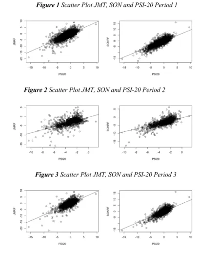
Figure 1 Scatter Plot JMT, SON and PSI-20 Period 1
Figure 2 Scatter Plot JMT, SON and PSI-20 Period 2
The scatter diagrams suggest a positive linear association between Jerónimo Martins and Sonae’s returns and PSI-20 returns: they tend to move in the same direction, meaning that a positive or negative variation of the PSI-20 index returns tends to be accompanied by a positive or negative variation of Jerónimo Martins and Sonae’s returns in the sample considered.
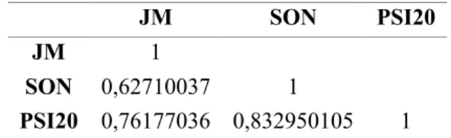
Table 1 Linear Correlation Coefficients
JM SON PSI20
JM 1
SON 0,62710037 1
PSI20 0,76177036 0,832950105 1
The value of the linear correlation coefficient confirms the strong positive linear association between the variables. The strongest relation is between the PSI-20 index and Sonae, since it is the closest value to 1.
To test if the sample linear correlation coefficient is statistically significant, we can perform the following test:
H0: ρ = 0
H1: ρ ¹ 0
where ρ is the population linear correlation coefficient.
Table 2 Correlation significance test
t-stat p-value
SON-JM 50,8151924 0
PSI20-JM 74,2183316 0
PSI20-SON 95,0123867 0
Based on the p-value obtained (0) we reject the null hypothesis. In all cases, the probability associated with the test value is always lower than the level of significance considered by default (α = 0.05), rejecting the null hypothesis that ρ = 0. Thus, we conclude that the correlation coefficients obtained are statistically significant, considering the sample used and the 0.05 significance level.
4.2. Estimation and statistical significance of the regression coefficients
The betas of each company were estimated through the simple linear regression during three different time periods.
After that, studies on the adequacy of the simple linear regression model were done, namely, checking the statistical significance for the alpha parameter (α) and for the beta parameter (β), analysing the coefficient of determination and the residuals.
Thus, betas were estimated in Period 1 based on 3986 observations of daily returns. After that, we divided this period in a pre-crisis period: Period 2 was based on 1252 observations of daily returns; and post-crisis period: Period 3, based on 2734 observations of daily returns.
The following tables show the estimated values for α, the respective values of the t statistic and the p-value.
Period 1
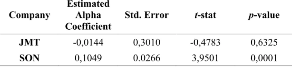
Table 3 Estimates and significance tests for alpha coefficient Period 1
Company
Estimated Alpha Coefficient
Std. Error t-stat p-value
JMT -0,0144 0,3010 -0,4783 0,6325
SON 0,1049 0.0266 3,9501 0,0001
Period 2
Table 4 Estimated alpha coefficients Period 2
Company
Estimated Alpha Coefficient
Std. Error t-stat p-value
JMT -0,3841 0.1094 -3,5122 0,0005
Period 3
Table 5 Estimated alpha coefficients Period 3
Company
Estimated Alpha Coefficient
Std. Error t-stat p-value
JMT 0,0200 0.0316 0,6333 0,5266
SON 0,0632 0.0275 2,3008 0,0215
The t statistic and the p-value were used to check the statistical significance of the alpha parameter (ordinate at origin) in the simple regression model.
Thus, to test the validity of CAPM, the intercept term should not be statistically significant in the model and the market risk premium term should be statistically significant and positive.
The results show that for Jerónimo Martins the values of the t-test for the alpha coefficient in period 1 and period 3 (-0,4783 and 0,6333) are inside the rejection zone: RR = ]-∞; -1.961] ∪ [1.961, ∞[, obtained through: t (0,975;3984) and t (0,975; 2732) respectively) and the respective p-values (0,6325 and 0,5266) are higher than the significance level α = 0.05. This means that we do not reject the null hypothesis (H0: α =
0), so, the estimate for alpha is not statistically significant.
The exception is in period 2, in which the value of the t-test (-3,5122) is outside the Rejection zone: RR = ]-∞; -1.962] ∪ [1.962, ∞[ and the respective p-value (0,005) is lower than the significance level α = 0.05. This means that we reject the null hypothesis (H0: α = 0), so, the estimate for alpha is statistically significant.
For Sonae, all the values of the t-test for the alpha coefficient in the three different time periods (3,9501; 5,2711 and 2,3008) are outside the rejection zone and the respective
p-values (0,0001; 0 and 0,0215) are lower than the significance level α = 0.05. Therefore
we reject the null hypothesis (H0: α = 0), meaning that the estimate for alpha is statistically significant.
The table below shows the estimates for β, the values of the t statistic and the respective p-values for the three different time periods.
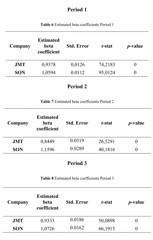
Period 1
Table 6 Estimated beta coefficients Period 1
Company
Estimated beta coefficient
Std. Error t-stat p-value
JMT 0,9378 0,0126 74,2183 0
SON 1,0594 0.0112 95,0124 0
Period 2
Table 7 Estimated beta coefficients Period 2
Company
Estimated beta coefficient
Std. Error t-stat p-value
JMT 0,8449 0.0319 26,5291 0
SON 1,1596 0.0289 40,1816 0
Period 3
Table 8 Estimated beta coefficients Period 3
Company
Estimated beta coefficient
Std. Error t-stat p-value
JMT 0,9333 0.0186 50,0898 0
SON 1,0726 0.0162 66,1915 0
Regarding the beta estimate for both Jerónimo Martins and Sonae, we reject the null hypothesis in the three different time periods, since the values of the t-test are outside the critical regions and the respective p-values (0) are lower than the significance level (0.05), meaning that the estimates for the beta coefficients are statistically significant. We can
conclude that there is a significant relationship between the independent and dependent variables.
Based on estimates for alpha and beta, the estimated equations are given by:
Table 9 Estimated equations for Jerónimo Martins
Period 1 𝐽𝑀~i = -0,0144 + 0,9378 PSI20i
Period 2 JM~i = -0,3841 + 0,8450 PSI20i
Period 3 JM~i = 0,0200 + 0,9333 PSI20i
Table 10 Estimated equations for Sonae
Period 1 𝑆𝑂𝑁Ti = 0,1049+ 1,0594 PSI20i
Period 2 SONTi = 0,5223 + 1,1596 PSI20i
Period 3 SONTi = 0,0632 + 1,0726 PSI20i
4.3. Analysing the systematic risk
After that, we analysed the coefficient of determination (R2), which is used as an
indicator of the goodness of fit.
Period 1
Table 11 Coefficient of Determination Period 1
Company Coefficient of Determination
(R2)
JMT 0,5803
Period 2
Table 12 Coefficient of Determination Period 2
Company Coefficient of Determination (R2)
JMT 0,3602
SON 0,5636
Period 3
Table 13 Coefficient of Determination Period 3
Company Coefficient of Determination
(R2)
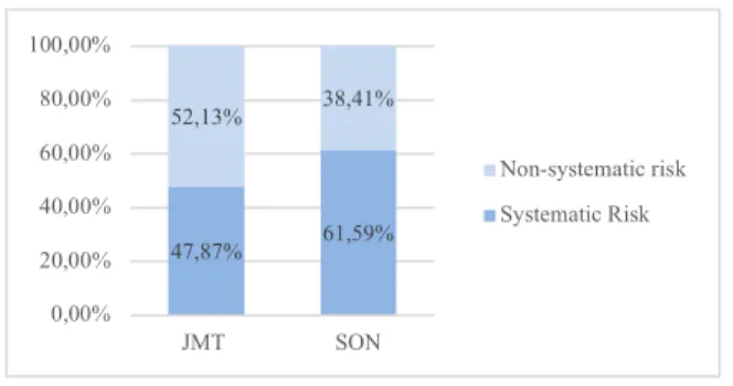
JMT 0,4787
SON 0,6159
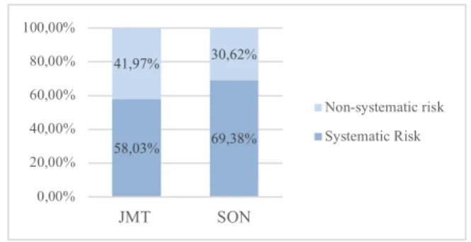
We know that the closer the R2 value is to 1, the better the model explains the
dependent. The R2 of Sonae is higher in the three different time periods. The highest value
of R2 is in period 1 and it is 0,6938, meaning that 69,38% of the total variability of y (the
riskless return of Sonae) is explained by x (the riskless market returns), and the remaining 30.62% are due to other factors.
The lowest R2 is from Jerónimo Martins, during period 2 and it is 0,3602, meaning
that the weight of the systematic risk in the total risk of Jerónimo Martins is 36,02%, and the remaining 63,98% are attributed to firm-specific factors of risk.
In the following charts we can see a comparison of the weights of the systematic and non-systematic risk in total risk.
Figure 4 Weight of the systematic and non-systematic risk in total risk Period 1
58,03% 69,38% 41,97% 30,62% 0,00% 20,00% 40,00% 60,00% 80,00% 100,00% JMT SON Non-systematic risk Systematic Risk
Figure 5 Weight of the systematic and non-systematic risk in total risk Period 2
Figure 6 Weight of the systematic and non-systematic risk in total risk Period 3
To calculate the systematic risk of the securities, we used the betas estimated through the regression, the market returns variation and the variation of the returns of each company.
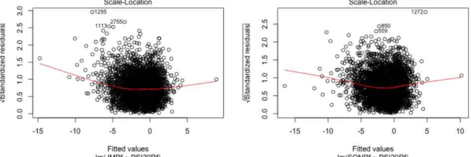
4.4. RESET test
The next step was testing if there was omission of relevant explanatory variables, incorrect functional form and correlation between explanatory variables and the errors of the model. To this end, we started by performing the RESET test (Regression Specification Error Test) to assess if one of the specification errors mentioned above occurred.
Table 14 P-values associated to the RESET test
JM PSI20 SON PSI20
Period 1 0.0017 0.1205 Period 2 0.0156 0.0787 Period 3 1.227e-05 0.39 36,02% 56,36% 63,98% 43,64% 0,00% 20,00% 40,00% 60,00% 80,00% 100,00% JMT SON Non-systematic risk Systematic Risk 47,87% 61,59% 52,13% 38,41% 0,00% 20,00% 40,00% 60,00% 80,00% 100,00% JMT SON Non-systematic risk Systematic Risk
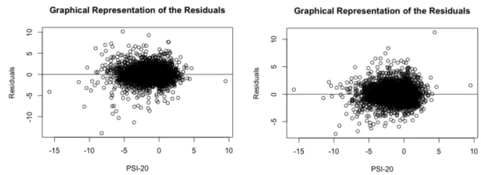
In all the three periods, for Jerónimo Martins and based on the p-value we reject the null hypothesis. This means that at least one of the three assumptions checked by the RESET test is violated. If we have a look at the following plots, we can see that some points are furthest away from the straight line, so one possible cause for the rejection of the null hypothesis could be the omission of variables.
Figure 7 Graphical Representation of the Residuals of JMT and SON against the PSI-20 Period 1
Figure 8Graphical Representation of the Residuals of JMT and SON against the PSI-20 Period 2
Figure 9 Graphical Representation of the Residuals of JMT and SON against the PSI-20 Period 3
Regarding Sonae, and since the p-values are higher than 0.05, we do not reject the null hypothesis, therefore none of the assumptions is violated.
There are several other assumptions that must be checked for the OLS estimators to be fulfilled, such as the linearity of the data, the normality of residuals, homoscedasticity and independence of error terms.
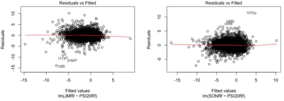
4.5. Linearity
We will start by checking the linearity assumption, that implies that the relationship between the predictor (x) and the outcome (y) is assumed to be linear. To this end, we can have a look in the plots Residuals vs Fitted.
Figure 10 Residuals vs Predicted values period 1
Figure 11 Residuals vs Predicted values period 2
The red line should be approximately horizontal near zero and should not show patterns. In our example, these conditions hold, which suggests that we can assume that there is a linear relationship between our variables.
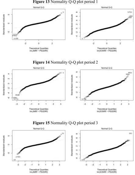
4.6. Normality of the errors
The next step was checking the errors' normality assumption, which is of utmost importance, since it is the support of all statistical inference in the linear regression model (F and the t-tests) for the estimated coefficients, especially when we have small samples.
We can have a look in the Normal Q-Q plots to check whether the residuals are normally distributed or not.
Figure 13 Normality Q-Q plot period 1
Figure 14 Normality Q-Q plot period 2